Exact ground state Monte Carlo method for Bosons without importance sampling
Abstract
Generally “exact” Quantum Monte Carlo computations for the ground state of many Bosons make use of importance sampling. The importance sampling is based, either on a guiding function or on an initial variational wave function. Here we investigate the need of importance sampling in the case of Path Integral Ground State (PIGS) Monte Carlo. PIGS is based on a discrete imaginary time evolution of an initial wave function with a non zero overlap with the ground state, that gives rise to a discrete path which is sampled via a Metropolis like algorithm. In principle the exact ground state is reached in the limit of an infinite imaginary time evolution, but actual computations are based on finite time evolutions and the question is whether such computations give unbiased exact results. We have studied bulk liquid and solid 4He with PIGS by considering as initial wave function a constant, i.e. the ground state of an ideal Bose gas. This implies that the evolution toward the ground state is driven only by the imaginary time propagator, i.e. there is no importance sampling. For both the phases we obtain results converging to those obtained by considering the best available variational wave function (the Shadow wave function) as initial wave function. Moreover we obtain the same results even by considering wave functions with the wrong correlations, for instance a wave function of a strongly localized Einstein crystal for the liquid phase. This convergence is true not only for diagonal properties such as the energy, the radial distribution function and the static structure factor, but also for off–diagonal ones, such as the one–body density matrix. This robustness of PIGS can be traced back to the fact that the chosen initial wave function acts only at the beginning of the path without affecting the imaginary time propagator. From this analysis we conclude that zero temperature PIGS calculations can be as unbiased as those of finite temperature Path Integral Monte Carlo. On the other hand, a judicious choice of the initial wave function greatly improves the rate of convergence to the exact results.
I INTRODUCTION
Among the available methods to investigate the properties of strongly interacting many–body quantum systems, Quantum Monte Carlo (QMC) ones hold a relevant position since some of the QMC methods can provide “exact” expectation values. As for all the Monte Carlo methods, QMC results are affected by statistical uncertainties, but the property that makes some of them “exact” is the possibility of reducing within this unavoidable errors all the systematic errors introduced by the involved approximations. This is true for Boson system at zero and at finite temperature, but the studies of Fermion systems, excited states or real time dynamics all suffer from sign problems which still have precluded the development of such kind of “exact” methods. A first great subdivision of “exact” QMC methods is between finite and zero temperature methods. Among K methods we find Green Function Monte Carlo (GFMC),[1, 2, 3] Diffusion Monte Carlo (DMC),[4] Path Integral Ground State Monte Carlo (PIGS)[5] and Reptation Monte Carlo (RMC).[6] At finite temperature, the major role is played by Path Integral Monte Carlo (PIMC).[7]
The main difference between finite and zero temperature methods is that ground state methods rely, to different extents, on a trial wave function for the importance sampling, while in PIMC no such wave function is involved at all. PIMC needs only information on the interaction among particles as input, and the main difficulty to overcome, beyond the propagator accuracy, is the sampling ergodicity. Recently a great step forward in this direction has been realized with the advent of the worm algorithm.[8] The first GFMC computation did not use importance sampling,[1] but this computation was for a small system of 32 particles. All the other computation at zero temperature have used a model wave function that was given as input. With respect to PIGS method, if , in principle, convergence can be achieved for any initial wave function that has a finite overlap with the ground state, the question is if convergence can be achieved in a real computation. Some progress have been achieved recently both for a finite[9] and for a bulk Boson system.[10] For example, a Jastrow wave function, that describes the bulk phase of a quantum liquid, was employed as initial wave function in the study of small parahydrogen clusters.[9] In the case of a two dimensional crystal of 4He, convergence to the same result was found in the computation of the one–body density matrix starting from two initial wave functions with “opposite” properties,[10] one with Bose–Einstein condensate and the other without. Stimulated by these results, we have undergone a systematic check for a realistic Hamiltonian for 4He and we have found that PIGS methods converge to the exact result regardless of the chosen initial wave function. Even better, PIGS converges even if the wave function contains wrong correlations or no correlations at all.
As a test–bed we have considered the bulk liquid and solid phases of a strongly interacting boson system such as 4He. By projecting very different wave functions, we find converging results for diagonal properties like the energy, the radial distribution function, the static structure factor and also for off-diagonal properties like the one-body density matrix. For both the liquid and the solid phases we consider a shadow wave function (SWF),[11] which is the best available variational wave function[12] for 4He systems, and the constant wave function (CWF), which is the ground state wave function of the ideal Bose gas and does not contain any correlation. The latter corresponds to have no importance sampling since the initial wave function gives the same weight to any configuration of the particles. Furthermore, for the liquid phase, we have considered also a localized wave function which describes an Einstein solid. Our question is whether PIGS is able to recover the exact ground state starting from really different systems, i.e. an ideal gas or an Einstein crystal for the quantum liquid and an ideal gas for the quantum solid. We find that for all the considered initial wave functions PIGS converges to the exact ground state. Only the convergence rate depends on the initial wave function, and turns out to be slower for the worse ones.
II METHOD
II.1 The PIGS method
It is well known that, given a Hamiltonian for a quantum system of particles, the ground state wave function in the position representation can be obtained as the limit of an imaginary time () evolution of an initial (trial) wave function , provided that :
| (1) |
Regardless of a normalization constant, which is not involved in the Monte Carlo sampling and thus will be dropped in the following, an accurate approximation of the ground state wave function is given by
| (2) |
This originates from the action of the imaginary time projector , which exponentially removes from any overlap with the excited states during the imaginary time evolution. The evolved wave function and Eq. (1) provide the basis for all the zero temperature QMC methods.
A first problem rises: the imaginary time propagator can be accurately written only for small values of , but a large limit is necessary to ensure the convergence to . One possible strategy to overcome this problem is to reach the large limit by means of a recursive procedure, as for example in GFMC[1] and DMC.[4] Both these methods reach an extremely accurate approximation of the ground state wave function multiplied by by iterating equation (1) by means of random walks. With these methods the trial wave function has a strategical role since it is involved at each iteration step, where it is used as importance sampling function.
On the contrary, the PIGS method[5] interprets the imaginary time propagator as a density matrix operator corresponding to an inverse temperature , and then, by exploiting the factorization property
| (3) |
the large propagator is written as a convolution of small imaginary time propagators as in standard path integral formalism.[5] Thus the density matrix operator is broken up into small pieces with a time step and the approximated ground state wave function reads
| (4) |
An appealing feature, peculiar of this method is that, in , the ansatz on acts only at the starting point being the full imaginary time path governed by , which depends only on . Once fixed , the elementary evolution step in imaginary time is obtained acting with on a quantum state; this action is usually called projection step due to the resulting increased overlap with the ground state. The PIGS method reaches convergence to the ground state when adding further imaginary time projections to does not provide any appreciable change of the results, i.e. the expectation values computed with is compatible with those computed with within the statistical errors for any integer . Since the convergence on the ground state for a finite system is exponentially fast,[13] the number of required imaginary time projections is usually limited. Nevertheless depends on the specific expectation value one is computing, thus a separate analysis of the convergence should be carried on for every computed quantity. The convergence rate is determined essentially by the quality of the initial wave function. The total imaginary time required to clean the initial wave function up from excited state contributions is smaller for good (i.e. with large overlap with the ground state) initial wave functions. Also the accuracy of the approximation used for the small time has a role in determining the computational cost of the projection procedure: in fact, with better approximations of the small imaginary time , one needs a smaller number of projection steps to reach convergence since larger time step are allowed. Moreover the imaginary time projection procedure should be able, in principle, to incorporate in the final wave function all the correct correlations, even if these were absent in . Thus it should be possible, in principle, to obtain the correct ground state wave function, if is large enough, even if is extremely poor, and the results do not suffer from any variational bias. The intent of the present study is to show that this is indeed the case with values of manageable with present computational resources.
Like for finite temperature PIMC,[7] also within PIGS the quantum system is mapped into a system of classical polymers, but in this case the polymers start and end on the initial wave function ,[5, 14, 15] resulting in open linear polymers instead of the close ring ones of PIMC.[7] Each open polymer represents the full imaginary time path of a quantum particle that is sampled by means of the Metropolis algorithm. Thus, the entire imaginary time evolution of the system is sampled at each Monte Carlo step, contrary to what happens for DMC, for example. Expectation values of an operator reads
| (5) |
and, if is large enough to allow convergence to the ground state, is the ground state expectation value, without needing any extrapolation. However an analysis of the convergence as a function of is needed, as explained before.
The ground state expectation value of the energy can be obtained in several ways: the most largely employed one is the mixed estimate
| (6) |
Notice that in PIGS this mixed estimate is exact. In fact, since the Hamiltonian operator commutes with the imaginary time evolution operator , it is possible to obtain unbiased expectation value of the Hamiltonian inserting at one of the ends of the path. If is an accurate wave function, this estimator is preferable with respect to the direct one given by Eq. (5) with , because it has typically a lower variance. This is no more true, however, when the initial wave function is particularly poor. In this case the fluctuations in the expectation value of the Hamiltonian become so sizable that (6) is unusable. The direct estimator is seldom used because one has to compute the first and the second derivative of ; but this is not a serious problem if the imaginary time propagator is available in an analytical formulation, like the one we employed here. When is a good wave function, as for the SWF case, we have verified that mixed and direct estimators provide compatible results, and we report here the mixed one for the above mentioned reason. On the contrary, for poor wave functions, like CWF, we had to consider the direct estimator.
As far as 4He systems are concerned, because of the Bose statistic obeyed by the atoms, one has, in principle, to account for permutations in the propagator .[5, 7] Permutation moves are not strictly requested whenever the initial wave function has the correct Bose symmetry. In fact, the polymer configuration resulting after a permutation can be in principle reached with a combination of standard sampling moves, since the polymers are open.[14, 15] This is not the case if is not Bose symmetric like the Gaussian wave function: permutation cycles among particles must be introduced in the sampling in order to get the exact ground state. For all we have implemented permutation sampling following Ref. 16. In fact, implementing the sampling of permutations even for a Bose symmetric turns out to greatly improve the ergodicity of the sampling. In addition, we have used swap moves[8] because they increase the sampling efficiency when computing off–diagonal properties.[10]
II.2 Test systems
In order to test the PIGS method convergence properties we have considered two bulk phases of a many–body strongly interacting Boson system: liquid and solid 4He. Dealing with low temperature properties, 4He atoms are described as structureless zero–spin bosons, interacting through a realistic two–body potential, that we assume to be the HFDHE2 Aziz potential [17]. For the liquid phase, we have considered a cubic box with periodic boundary conditions, containing atoms at the equilibrium density Å-3. For the solid phase we have considered a cubic box with periodic boundary conditions designed to house a fcc crystal of atoms at the density Å-3. In both cases we add standard tail corrections to the potential energy to account for the finite size of the system by assuming the medium homogeneous (i.e. ) beyond , where is the size of the box. Obviously, this is not an accurate assumption specially for the solid phase in such a small box, but our main purpose here is to show that PIGS method is able to reach the same results independently on the considered initial wave function. Moreover we have studied the fcc lattice, which is stabilized by the cell geometry and by the periodic boundary conditions, whereas at zero temperature, the hcp lattice is the stable lattice. Computations of ground state properties of bulk 4He with accurate tail corrections can be found in the current literature.[18, 12]
II.3 Initial wave functions
The standard initial wave functions commonly used within PIGS method[5] are the variational Jastrow wave function (JWF) for the liquid and the Jastrow-Nosanow (J-NWF) for the solid. A JWF represents the simplest possible choice of wave function for strongly interacting Bosons[19] and it contains only two–body correlations. Using a McMillan pseudopotential,[20] the unnormalized JWF reads as
| (7) |
The physical meaning of this JWF is that, due to the sharp repulsive part of the interaction potential in the Hamiltonian , 4He atoms prefer to avoid each other. In the J-NWF the JWF is multiplied by a term like the one in Eq. (10) below, that localizes the particles in a crystalline order. In this work, however, in order to explore the convergence properties of the PIGS method, we have considered two wave functions of “opposite” quality: the best available one, that is the shadow wave function, and the poorest imaginable one, i.e. the constant wave function. JWF will be considered only when computing the one–body density matrix in the liquid phase.
The constant wave function is the ground state wave function of the ideal Bose gas,
| (8) |
It carries no correlation at all. We choose this wave function because, allowing an unrestricted sampling of the full configurational space, it results in no importance sampling. Then the whole imaginary time projection procedure is driven only by the short time evolution operator , without any input, and then any bias, from the initial state. Thus at the starting point the system is made up by free particles; if after a long enough imaginary time projection, PIGS turns out to be able to reach a strong correlated quantum liquid and quantum crystal by itself we can safely believe that no variational bias affects PIGS results.
On the other hand, we choose as a SWF given by variational computation in order to have as reference results the ones coming from the projection of an initial wave function that is more accurate as possible, i.e. from a wave function whose overlap with the exact ground state is known to be large. In the SWF, additional correlations besides the standard two body terms are introduced via auxiliary variables which are integrated out.[11] This is done so efficiently that the crystalline phase emerges as a spontaneously broken symmetry process, induced by the inter–particles correlations as the density is increased, without the need of any a priori knowledge of the equilibrium positions and without losing the translationally invariant form of the wave function. Thus SWF is able to describe both the liquid and the solid phase with the same functional form and it is explicitly Bose symmetric. The standard SWF functional form reads
| (9) |
where is the set of auxiliary shadow variables, is the standard Jastrow two body correlation term (7), is a kernel coupling each shadow to the corresponding real variable, and is another Jastrow term describing the inter–shadow correlations. As usual,[21] we take Gaussian and in we use the rescaled and dilated He–He potential as pseudopotential. The variational parameters we use were chosen in order to minimize the expectation value of the Hamiltonian and are reported in Ref. 21. Nowadays the SWF represents the best available variational wave function for 4He systems.[12] Recently, we have estimated[10] that, when describing a two dimensional solid, SWF overlap per particle with the true ground state is of about 99.8%, which ensures a fast convergence rate when projected within the PIGS method. The properties of the SWF are so peculiar that the PIGS method that has a SWF as deserves an its own name and is dubbed SPIGS: Shadow Path Integral Ground State method.[14, 15] In the picture of linear polymers, the presence of the shadow variables adds two extra variational links, one at each end of the polymer.
In order to test how robust PIGS is, we consider also a “wrong” wave function: for the liquid phase we consider a Gaussian wave function, where each particle is harmonically localized around fixed positions
| (10) |
i.e. it the wave function of an Einstein harmonic solid. The parameter Å-2 is arbitrary and it is was chosen to ensure a strong localization of the particles around the positions that were taken over a regular cubic lattice within the simulation box. This wave function is evidently not translationally invariant and not Bose symmetric. Furthermore it does not contain any correlation between the particles, and all the information that it carries is that of a crystalline system, i.e. GWF is an extremely poor wave function for the liquid phase. This wrong initial wave function will provide a stringent test on the convergence properties of the PIGS methods.
As far as the one–body density matrix computation in the liquid phase is concerned, the values of the parameters and in the JWF have been chosen equal to the ones of the corresponding Jastrow term in the SWF.
II.4 Small time propagator
One of the fundamental elements of path integral projection Monte Carlo methods is the imaginary time propagator , whose accuracy turns out to be crucial to the convergence to the exact results. The functional form of for a generic is unfortunately not known with exception of few particular cases, such as, for example, the free particle and the harmonic oscillator, but accurate approximations of are obtainable in the small regime.[7, 13, 22] In this work, we have chosen the Pair–Suzuki approximation[23] for the imaginary time propagator, which is a pair–approximation of the fourth–order Suzuki–Chin density matrix.[13]
The Suzuki–Chin approximation is based on the following factorization of the density matrix:
| (11) |
where is the kinetic operator and and are given by
| (12) |
and
| (13) |
respectively, with the potential operator, an arbitrary constant in the range , and . The resulting imaginary time propagator is accurate to order , and has been successfully applied to liquid 4He in two and three dimensions.[13] This approximation offers also the advantage that adjusting the parameter it is possible to optimize the convergence, and a standard choice for a quantum system is .[13] A strategy to obtain a simpler, but equally accurate, approximation consists in applying a pair product assumption.[23] For sufficiently short time steps, in fact, the many–body propagator (in imaginary time) is well approximated by the product of two–body propagators.[7] In this approximation, the small time propagator reads
| (14) |
where is given as
| (15) |
The potentials and are defined as
| (16) |
where is the potential experienced by two 4He atoms at a distance . The advantage is that there is no need to calculate . As for the full Suzuki–Chin approximation,[13] also for the Pair–Suzuki the operators corresponding to physical observables must be inserted only on odd time slices in the imaginary time path.

In order to fix the optimal small imaginary time step value, we have performed PIGS simulations with different initial wave functions. By considering decreasing values with a fixed total projection time, , we have taken the energy per particle as observable of reference. As an example, our results for SWF and CWF in the liquid phase are plotted in Fig. 1. We choose as optimal value K-1; in fact, further reductions do not change the energy in a detectable way, i.e. within the statistical uncertainty. In Fig. 1 SWF and CWF do not converge to the same value simply because the considered total projection time in this test is not enough to ensure convergence of to the ground state energy for CWF (see Fig. 2). Similarly, in the solid phase we take K-1.
III RESULTS
Once set the optimal value, we have computed the diagonal properties of the system for increasing total projection time until we reached convergence to a value that corresponds to the exact ground state result both for the liquid and for the solid phase. In the liquid phase we have computed also the one–body density matrix.
III.1 Liquid
III.1.1 PIGS results without importance sampling
For the liquid phase we have projected a SWF and a CWF. The energy per particle as a function of the total projection time for both the wave functions is plotted in Fig. 2.

We find that the energy converges, independently from the considered initial wave function, to the same value K. This value, in spite of the small size of the considered system, is close to the experimental[24] result K. SWF converges very quickly, in fact K-1 is already enough to ensure convergence. CWF instead, requires a three times larger imaginary time, i.e. K-1. This was somehow expected, since SWF is presently the best available variational wave function for 4He.[12] Nevertheless, the quick convergence of also CWF is a really remarkable result. In fact, this means that PIGS efficiently includes the exact interparticle correlations through the imaginary time projections, without any need of importance sampling. Then, the choice of a good wave function, within the PIGS method, becomes a matter of convenience rather than of principle, since better initial wave functions only allow for a smaller total projection time , and thus less CPU consuming simulations.


This convergence is confirmed also by the radial distribution function and the static structure factor . For such quantities, the convergence rate is found to be similar to the energy one. In Fig. 3 we report the radial distribution function obtained by projecting both a SWF and a CWF at different imaginary time values. For K-1, SWF results at different are indistinguishable within the statistical uncertainty (see Fig. 3a). In fact, with SWF the exact result is reached within very few projection steps and then it is no more affected by further projections. As already pointed out, also CWF displays a fast convergence, as shown in Fig. 3c, where is shown. For increasing , evolves toward a flat function, meaning that the systems described starting from the two different wave functions, i.e the strongly correlated quantum liquid of SWF and the ideal gas of CWF, are evolving into the same quantum liquid, which is the best reachable representation of the exact ground state of the simulated system. The same conclusion is inferred from the evolution of the static structure factor , which is plotted in Fig. 4.
III.1.2 PIGS results from a wrong initial function
In order to put a more stringent check on the PIGS method ability to converge to the exact ground state without any variational bias, we have considered also a wrong initial wave function by projecting a GWF. Thus at the starting point of the imaginary time path there is now a strongly localized Einstein crystal. We find, even in this case, that the energy converges to the same value as before (see Fig. 2). Thus PIGS is able not only to drop from the initial wave function the wrong information of localization, but also to generate at the same time the correct correlations among the particles. GWF needs K-1 to converge, which is ten times larger than the SWF value.


Again this convergence is confirmed also by the radial distribution function and the static structure factor . In Fig. 5 we report the radial distribution function obtained by projecting a GWF at different imaginary time values compared with the ones coming from the projection of SWF. It is evident that small imaginary time is not enough to leave out the wrong information in the GWF. For lower values, there are still reminiscences of the starting harmonic solid, which are progressively lost as the projection time increases. This is made clearer in Fig. 5b where we plot the difference , at fixed imaginary time , between the computed by projecting the SWF and the one obtained by projecting the GWF. A similar behavior is observed in the evolution static structure factor , plotted in Fig. 6. For the GWF, the Bragg peak shown at small values (Fig. 6a), which is typical of the solid phase, becomes lower and lower as the projection time is increased (Fig. 6b), until convergence is reached (see Fig. 6c).
From the plot of the energy per particle vs. the total imaginary time it is possible to estimate the overlap per particle of the initial wave function on the exact ground state.[25] By using the results in Fig. 2 we find that the overlap of SWF is about 99%, while the GWF one is about 10%. That SWF has an high overlap with the ground state is not a surprise; it was qualitatively expected since SWF is presently the best available wave function for 4He.[12] However a 99% overlap is really remarkable and provides a further argument on the goodness of SWF. On the other hand, a poor overlap of GWF was somehow expected, since the parameter was chosen to strongly localize the atoms of the bulk liquid around fictitious equilibrium positions on a regular lattice.
III.1.3 Off-diagonal properties
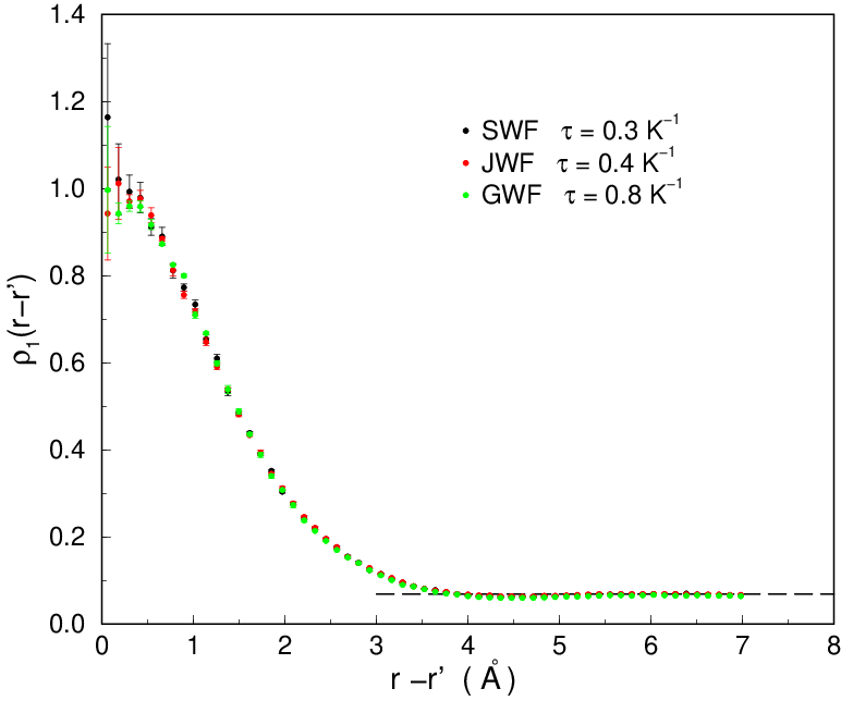
Besides the diagonal ones, also off–diagonal properties, such as the one–body density matrix, are accessible within PIGS simulations. The one-body density matrix represents the probability amplitude of destroying a particle in and creating one in . Its Fourier transformation represents the momentum distribution. In first quantization is given by the overlap between the normalized many-body ground state wave functions and , where the configuration differs from only by the position of one of the atoms in the system. If is translationally invariant, only depends on the difference , thus
| (17) |
The Bose-Einstein condensate fraction is equal to the large distance limit of . In fact, if has a nonzero plateau at large distance, the so called off-diagonal long-range order (ODLRO), its FT contains a Dirac delta function, which indicates a macroscopic occupation of a single momentum state, i.e. Bose–Einstein condensation.
The exact can be obtained in PIGS simulation by substituting in (17) with with large enough. This corresponds to the simulation of a system of linear polymers plus a polymer which is cut into two halfs, called half–polymers, one departing from and the other from . Thus is obtained by collecting the relative distances among the cut ends of the two half–polymers during the Monte Carlo sampling. The present computation of has been obtained by implementing a zero temperature version of the worm algorithm.[8] We have worked with a fixed number of particles and not in the grand canonical ensemble, similarly to what has been done at finite temperature in Ref. 23. In practice this corresponds to a usual PIGS calculation of where “open” and “close” moves have been implemented[8] in order to visit diagonal and off-diagonal sectors within the same simulation. The advantage of doing this does not come from the efficiency of the worm algorithm to explore off-diagonal configurations, because similar efficiency is obtained with PIGS when “swap” moves are implemented.[10] The benefit in using a worm-like algorithm here instead comes from the automatic normalization of which is a peculiarity of this method.[8] In Fig. 7 we report obtained in PIGS simulations of bulk liquid 4He at Å-3 by projecting either a SWF, a JWF and a GWF. All the simulations give the same result, shown in Fig. 7 which turns out to be compatible with the recent estimate obtained with PIGS given in Ref. 26 of .
III.2 Solid


We have performed the computation at density Å-3, where 4He is in the solid phase, by projecting a SWF and a CWF. Our results for the energy per particle are plotted in Fig. 8 as a function of . In both cases we find convergence to the value K. Even in this phase the convergence of SWF is faster, being K-1 enough to reach convergence. In the case of CWF convergence is reached only for a much larger imaginary time K-1.
Also in this case convergence is obtained for the radial distribution function and for the static structure factor, reported in Fig. 9 and Fig. 10 respectively. From Fig.9a it is evident that SWF has reached the true ground state with few projection steps, since the results for at K-1 and K-1 are indistinguishable. The evolution toward the correct ground state of the projected CWF is instead detectable. The presence of the crystalline structure is mainly evident in the static structure factor, where a Bragg peak grows with increasing (see Fig. 10a,b). The emerging of the correct solid structure by projecting a really poor wave function such as the CWF is made evident by the trend toward a flat function of the differences and plotted in Fig.9c and Fig.10c respectively.
IV CONCLUSION
In this work we have studied with the Path Integral Ground State method diagonal and off-diagonal properties of a strongly interacting quantum Bose system like the bulk liquid and solid phases of 4He. We have obtained convergence to the ground state values of quantities like the total energy, the radial distribution function, the static structure factor and the one-body density matrix projecting radically different wave functions: equivalent expectation values in the liquid phase have been obtained using as initial wave function a shadow wave function, a Gaussian wave function with strongly localized particles of an Einstein solid without interparticle correlations and also a constant wave function where all configurations of the particles are equally probable. Similarly in the solid phase equivalent expectation values have been obtained by considering a shadow wave function, which describes a solid, and a constant wave function which describes an ideal Bose gas. The present analysis demonstrates the absence of any variational bias in PIGS; a method that can be thus considered as unbiased as the finite temperature PIMC. This remarkable property comes from the accurate imaginary time propagators, exactly the same used with PIMC, that do not depend on the initial trial state. It remains true that the use of a good variational initial wave function greatly improves the rate of convergence to the exact results. Moreover, very poor wave functions have also the drawback of requiring the direct estimator for the Hamiltonian (Eq. (5) with ) implying the necessity of an analytical formulation for the small imaginary time propagator or an accurate knowledge of its derivatives.
We have addressed here only the case of a realistic interaction potential among Helium atoms. However one can reasonably expect that this conclusion holds even for very different kinds of interaction, once an accurate approximation for the imaginary time propagator is known (for example hard-spheres[27] or hydrogen plasma[28]). As far as pathological potentials like the attractive Coulomb one are concerned, PIGS would suffer the same limitations of PIMC if inaccurate approximations of the propagator were used.[29]
V ACKNOWLEDGMENTS
Authors acknowledge S. Pilati for useful discussions. This work was supported by the INFM Parallel Computing Initiative, by the Supercomputing facilities of CILEA and by the Mathematics Department “F. Enriques” of the Università degli Studi di Milano.
References
- [1] M.H. Kalos, Phys. Rev. A 2, 250 (1970).
- [2] M.H. Kalos, D. Levesque and L. Verlet, Phys. Rev. A 9, 2178 (1974).
- [3] P.A. Whitlock, D.M. Ceperley, G.V. Chester and M.H. Kalos, Phys. Rev. B 19, 5598 (1979).
- [4] P.J. Reynolds, D.M. Ceperley, B.J. Alder and W.A. Lester, J. Chem. Phys. 77, 5593 (1982).
- [5] A. Sarsa, k.E. Schmidt and W.R. Magro, J. Chem. Phys. 113, 1366 (2000).
- [6] S. Baroni and S. Moroni, Phys. Rev. Lett. 82, 4745 (1999).
- [7] D.M. Ceperley, Rev. Mod. Phys. 67, 279 (1995).
- [8] M. Boninsegni, N.V. Prokof’ev and B.V. Svistunov, Phys. Rev. Lett. 96, 070601 (2006); Phys. Rev. E 74, 036701 (2006).
- [9] J.E. Cuervo and P.-N. Roy, J. Chem. Phys. 125, 124314 (2006).
- [10] E. Vitali, M. Rossi, F. Tramonto, D.E. Galli and L. Reatto, Phys. Rev. B 77, 180505(R) (2008).
- [11] S.A. Vitiello, K. Runge and M.H. Kalos, Phys. Rev. Lett. 60, 1970 (1988).
- [12] S. Moroni, D.E. Galli, S. Fantoni and L. Reatto, Phys. Rev. B 58, 909 (1998).
- [13] J.E. Cuervo, P.-N. Roy and M. Boninsegni, J. Chem. Phys. 122, 114504 (2005).
- [14] D.E. Galli and L. Reatto, Mol. Phys. 101, 1697 (2003); J. Low Temp. Phys.
- [15] D.E. Galli and L. Reatto, J. Low Temp. Phys. 136, 343 (2004).
- [16] M. Boninsegni, J. Low Temp. Phys. 141, 27 (2005).
- [17] R.A. Aziz, V.P.S. Nain, J.S. Carley, W.L. Taylor and G.T. McConville, J. Chem. Phys. 70, 4330 (1979).
- [18] See for example J. Boronat and J. Casulleras, Phys. Rev. B 49, 8920 (1994).
- [19] see for instance, E. Feenberg, Theory of Quantum Fluids (Academic, New York, 1969).
- [20] W.L. McMillan, Phys. Rev. 138, A442 (1965).
- [21] T. MacFarland, S.A. Vitiello, L. Reatto and G.V. Chester, Phys. Rev. B 50, 13577 (1994).
- [22] K. Sakkos, J. Casulleras and J. Boronat, arXiv:0903.2763.
- [23] S. Pilati, PhD thesis Trento University, Italy (2008).
- [24] P.T. Roach, J.B. Ketterson and C.W. Woo, Phys. Rev. A 2, 543 (1970).
- [25] C. Mora and X. Waintal, Phys. Rev. Lett. 99, 030403 (2007).
- [26] S. Moroni and M. Boninsegni, J. Low Temp. Phys. 136, 129 (2004).
- [27] J. Cao and B.J. Berne, J. Chem. Phys. 97, 2382 (1992); L.M. Sesè and R. Ledesma, J. Chem. Phys. 102, 3776 (1995); P. Grüter, D.M. Ceperley and F. Laloë, Phys. Rev. Lett. 79, 3549 (1997).
- [28] C. Pierleoni, D.M. Ceperley, B. Bernu and W.R. Magro, Phys. Rev. Lett. 73, 2145 (1994).
- [29] M.H. Müser and B.J. Berne, J. Chem. Phys. 107, 571 (1997).