Velocity Curve Analysis of the Spectroscopic Binary Stars V373 Cas, V2388 Oph, V401 Cyg, GM Dra, V523 Cas, AB And, and HD 141929 by Artificial Neural Networks
Abstract
We used an Artificial Neural Network (ANN) to derive the orbital parameters of spectroscopic binary stars. Using measured radial velocity data of seven double-lined spectroscopic binary systems V373 Cas, V2388 Oph, V401 Cyg, GM Dra, V523 Cas, AB And, and HD 141929, we found corresponding orbital and spectroscopic elements. Our numerical results are in good agreement with those obtained by others using more traditional methods.
Key words. stars: binaries: eclipsing — stars: binaries: spectroscopic
1 Introduction
Determining the orbital elements of binary stars helps us to obtain fundamental information, such as the masses and radii of individual stars, that has an important role in understanding the present state and evolution of many interesting stellar objects. Analyzing of both light and radial velocity (hereafter RV) curves, derived from photometric and spectroscopic observations, respectively, yields a complete set of basic absolute parameters.
There are different methods to determine the orbit of a spectroscopic binary from its RV curve. Lehmann-Filhés (1894) introduced a geometrical method to determine the orbital elements from the geometrical properties of the RV curve, especially its maxima and minima. The method of Lehmann-Filhés has been found to be very useful, and little, if any, longer than other methods, providing a planimeter is used. This method also gives, for improving the final solution of the orbit, the differential corrections to the preliminary elements using the form of the equations of condition obtained by the method of least squares (see also Petrie 1960). Sterne (1941) described two forms of least square solutions. The first form is suitable for all orbits except those with very small eccentricities. The second form is particularly suitable for orbits having very small eccentricities (see also Petrie 1960). Karami Teimoorinia (2007) introduced a new non-linear least squares velocity curve analysis technique for spectroscopic binary stars. Their method was applicable to orbits of all eccentricities and inclination angles and the time consumed was considerably less than the method of Lehmann-Filhés. They showed the validity of their new method to a wide range of different types of binary. See Karami Mohebi (2007a,b) and Karami et al. (2008).
In the present paper, we use an Artificial Neural Network (ANN) to find the optimum match to the four parameters of the RV curves of the seven double-lined spectroscopic binary systems: V373 Cas, V2388 Oph, V401 Cyg, GM Dra, V523 Cas, AB And, and HD 141929. Our aim is to show the validity of our new method for a wide range of different binary types.
The spectral type of the primary and secondary component of V373 Cas is B0.5II and B4III, respectively. The mean effective temperature is 22000 and 18000 for the primary and secondary components. The angle of inclination is with a period of 13.4 days (Hill Fisher 1987). V2388 Oph is very close visual binary. The spectral type is F3 V with a relatively long period of 0.802 days. The system appears to be one of the most luminous among currently known contact binaries. Orbital inclination angle is (Rucinski et al. 2002). V401 Cyg appears to be a rather typical contact system. The orbital period is 0.582714 days (Rucinski et al. 2002). GM Dra is a contact system of the W-type, with spectral type F5V and period 0.338741 days (Rucinski et al. 2002). V523 Cas is one of the faintest known contact binaries. The spectral type is K4V and the period is 0.233693 days (Rucinski et al. 2003). AB And is a contact binary with spectral type G8V and period 0.3318919 days (Pych et al. 2004). HD 141929 is a double-lined spectroscopic binary with a period of 49.699 days. The orbit is eccentric (). The effective temperature for both components is estimated to . Both components have the same spectral type A0/1V, however, the secondary is rotating slower than the primary and the inclination of the orbit is about 11∘ (Carrier 2002).
Following Smart (1990), the radial velocity of a star in a binary system is defined as follows
| (1) |
where is the radial velocity of the center of mass of system with respect to the sun. Where , and are the angular polar coordinate (true anomaly), the longitude of periastron and the eccentricity, respectively. Also
| (2) |
where is the period of motion, is the semimajor axis of the orbit and inclination is the angle between the line of sight and the normal of the orbital plane.
From Smart (1990) for a small eccentricity, , the true anomaly, , can be expressed in terms of the photometric phase, , as follows
| (3) | |||||
Here we apply the ANN method to estimate the four orbital parameters, , , and of the RV curve in Eq. (1). ANNs have become a popular tool in almost every field of science. In recent years, ANNs have been widely used in astronomy for applications such as star/galaxy discrimination, morphological classification of galaxies, and spectral classification of stars (see Bazarghan et al. 2008 and references therein). Following Bazarghan et al. (2008), we employ Probabilistic Neural Networks (PNNs). An example of a PNN is shown in Fig. 1. This network has been investigated in ample details by Bazarghan et al. (2008).
In this work, for the identification of the observational RV curves, the input vector in Fig. 1, , is the fitted RV curve of a star with data points . This number is enough to cover the whole of RV curve. The network is first trained to classify RV curves corresponding to all the possible combinations of , , and . For this we synthetically generate RV curves given by Eq. (1). We generate one RV curve for each combination of the parameters:
- •
in steps of 1;
- •
in steps of 1;
- •
in steps of 0.001;
- •
in steps of 5.
Note that from Petrie (1960), one can guess , and from a RV curve. This enable us to limit the range of parameters around their initial guesses. This gives a set of pattern groups, one group for each combination of , , and . Each pattern group, , is characterized by Gaussian functions (see Bazarghan et al. 2008). For each system, we first fit a curve on the observational RV data. Then using the fitted curve, the RV is computed in photometric phases. When a observational RV curve of an unknown classification is fed to the network, the summation layer of the network computes the probability functions of each class. Finally at the output layer we have C, the value with the highest probability (see again Fig. 1).
2 Numerical Results
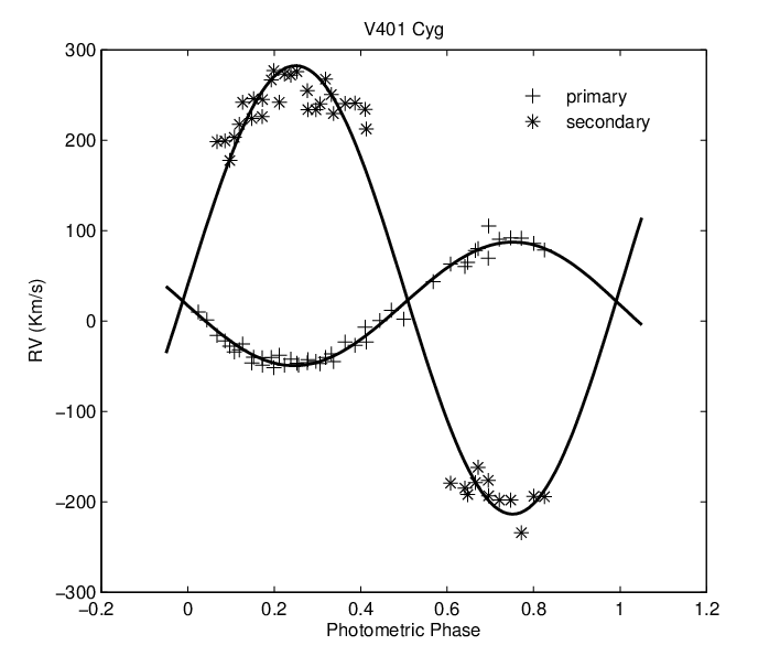
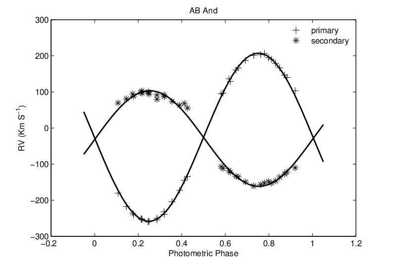
Here PNN is used as a tool to derive the orbital parameters of the seven different double-lined spectroscopic systems V373 Cas, V2388 Oph, V401 Cyg, GM Dra, V523 Cas, AB And, and HD 141929. Using measured RV data of the two components of these systems obtained by Hill & Fisher (1987) for V373 Cas, Rucinski et al. (2002) for V2388 Oph, V401 Cyg and GM Dra, Rucinski et al. (2003) for V523 Cas, Pych et al. (2004) for AB And, and Carrier (2002) for HD 141929, the fitted velocity curves are plotted in terms of the photometric phase in Figs. 2 to 8.
The orbital parameters obtaining from the ANN for V373 Cas, V2388 Oph, V401 Cyg, GM Dra, V523 Cas, AB And, and HD 141929 are tabulated in Tables 1, 3, 5, 7, 9, 11 and 13, respectively. Tables show that the results are in good accordance with the those obtained by aforementioned authors. Tables 9 and 11 show that the results of eccentricities for V523 Cas and AB And are not significantly different from zero. A Monte Carlo analysis clears that they should really be assigned circular orbits.
The combined spectroscopic elements including , , and are calculated by substituting the estimated parameters , and into Eqs. (3), (15) and (16) in Karami Teimoorinia (2007). The results obtained for the seven systems are tabulated in Tables 2, 4, 6, 8, 10, 12 and 14 show that our results are in good agreement with the those obtained by aforementioned authors.
Note that the errors in the tables of orbital parameters and combined spectroscopic elements in Karami & Mohebi (2009) seem to be unrealistic errors. But they are indeed the standard errors which are obtained from the nonlinear least squares of Eq. (14) in Karami & Teimoorinia (2007). The errors of observational RV data are not included in them. Following Lucy Sweeney (1971) the meaningful errors corresponding to the orbital elements , respectively, can be obtained from the inverse of the error diagonal matrix as with , , and . Where is the standard error of an observation of average weight. Using Eqs. (3), (15) and (16) in Karami Teimoorinia (2007), the errors of combined spectroscopic elements are obtained from the errors of orbital parameters.
3 Conclusions
An Artificial Neural Network to derive the orbital elements of spectroscopic binary stars is applied. This method is applicable to orbits of all eccentricities and inclination angles of different types of binaries. In this method the time consumed is considerably less than the method of Lehmann-Filhés and even less than the non-linear regression method introduced by Karami Teimoorinia (2007). It is possible to make adjustments in the elements before the final result is obtained. There are some cases, for which the geometrical methods are inapplicable, and in these cases the present one may be found useful. One such case would occur when observations are incomplete because certain phases could not have been observed. Another case in which this method is useful is that of a star attended by two dark companions with commensurable periods. In this case the resultant velocity curve may have several unequal maxima and the geometrical methods fail altogether.
Using the measured RV data of V373 Cas, V2388 Oph, V401 Cyg, GM Dra, V523 Cas, AB And, and HD 141929 given by aforementioned authors, we find the orbital elements of these systems by the PNN. Our numerical results shows that the results obtained for the orbital and spectroscopic parameters are in good agreement with those obtained by others using more traditional methods.
Acknowledgments
The authors wish to thank Graham Hill who his elaborate and meticulous comments has significantly improved the content and the presentation of the paper. This work has been supported financially by Research Institute for Astronomy Astrophysics of Maragha (RIAAM), Maragha, Iran.
References
- [1] Bazarghan, M., Safari, H., Innes, D.E., Karami, E. & Solanki, S.K., 2008, AA, 492, L13
- [2] Carrier, F., 2002, A&A, 389, 475
- [3] Hill, G. & Fisher, W. A., 1987, A&A, 171, 123
- [4] Petrie, R.M., 1960, Astronomical Techniques, ed. W.A. Hiltner, University of Chicago Press, Chicago
- [5] Karami, K. & Mohebi, R., 2007a, ChJAA, 7, 558
- [6] Karami, K. & Mohebi, R., 2007b, JApA, 28, 217
- [Karami, K. & Teimoorinia, H., 2007, Ap&SS, 311, 435] Karami, K. & Teimoorinia, H., 2007, Ap&SS, 311, 435
- [7] Karami, K., Mohebi, R. & Soltanzadeh, M.M., 2008, Ap&SS, 318, 69 (astro-ph/0808.1839v1)
- [8] Karami, K. & Mohebi, R., 2009, JApA (in press)
- [9] Lehmann-Filhés, R., 1894, AN, 136, 17
- [10] Lucy, L.B. & Sweeney, M.A., 1971, AJ, 76, 544
- [11] Pych, W., Rucinski, S.M., Debond, H., Thomson, J.R., Capobianco, C.C., Blake, R.M., Ogloza, W., Stachowski, G., Rogoziecki, P. & Gazeas, K., 2004, AJ, 127, 1712 (astro-ph/0311350)
- [12] Rucinski, S.M., Lu, W., Capobianco, C.C., Mochnacki, S.W., Blake, R.M., Thomson, J.R., Ogloza, W. & Stachowski, G., 2002, AJ, 124, 1738 (astro-ph/0201213)
- [13] Rucinski, S.M., Capobianco, C.C., Lu, W., Debond, H., Thomson, J.R., Mochnacki, S.W., Blake, R.M., Ogloza, W., Stachowski, G. & Rogoziecki, P., 2003, AJ, 125, 3258 (astro-ph/0302399)
- [14] Smart, W.M., 1990, Textbook on Spherical Astronomy, 6th edn. Cambridge University Press, Cambridge (revised by Green, R.M.), p. 360
- [15] Sterne, T.E., 1941, PNAS, 27, 175





| This Paper | Karami & Mohebi (2009) | Hill Fisher (1987) | |
|---|---|---|---|
| Primary | |||
| – | |||
| – | |||
| Secondary | |||
| – | |||
| – | |||
| – | |||
| – |
| Parameter | This Paper | Karami & Mohebi (2009) | Hill Fisher (1987) |
|---|---|---|---|
| This Paper | Karami & Mohebi (2009) | Rucinski et al. (2002) | |
|---|---|---|---|
| Primary | |||
| – | |||
| – | |||
| Secondary | |||
| – | |||
| – |
| Parameter | This Paper | Karami & Mohebi (2009) | Rucinski et al. (2002) |
|---|---|---|---|
| – | |||
| – | |||
| – | |||
| This Paper | Karami & Mohebi (2009) | Rucinski et al. (2002) | |
|---|---|---|---|
| Primary | |||
| – | |||
| – | |||
| Secondary | |||
| – | |||
| – |
| Parameter | This Paper | Karami & Mohebi (2009) | Rucinski et al. (2002) |
|---|---|---|---|
| – | |||
| – | |||
| – | |||
| This Paper | Karami & Mohebi (2007a) | Rucinski et al. (2002) | |
|---|---|---|---|
| Primary | |||
| — | |||
| — | |||
| Secondary | |||
| — | |||
| — |
| Parameter | This Paper | Karami & Mohebi (2007a) | Rucinski et al. (2002) |
|---|---|---|---|
| — | |||
| — | |||
| — | |||
| This Paper | Karami & Mohebi (2009) | Rucinski et al. (2003) | |
|---|---|---|---|
| Primary | |||
| – | |||
| – | |||
| Secondary | |||
| – | |||
| – |
| Parameter | This Paper | Karami & Mohebi (2009) | Rucinski et al. (2003) |
|---|---|---|---|
| – | |||
| – | |||
| – | |||
| This Paper | Karami et al. (2008) | Pych et al. (2004) | ||
|---|---|---|---|---|
| Primary | ||||
| — | ||||
| — | ||||
| Secondary | ||||
| — | ||||
| — |
| Parameter | This Paper | Karami et al. (2008) | Pych et al. (2004) |
|---|---|---|---|
| — | |||
| — | |||
| — | |||
| This Paper | Karami & Mohebi (2007b) | Carrier (2002) | |
|---|---|---|---|
| Primary | |||
| Secondary | |||
| Parameter | This paper | Karami & Mohebi (2007b) | Carrier (2002) |
|---|---|---|---|