Exact ground states and correlation functions of chain and ladder models of
interacting hardcore bosons or spinless fermions

In this subsection, our goal is to establish the one-to-one correspondence between states of the excluded and ordinary chains, and to show that as matrices, the Hamiltonians (1) and (3) are identical. To do this, let us note that an excluded chain with $L$ sites has fewer $P$-particle states than an ordinary chain of $L$ sites, because of the infinite nearest-neighbor repulsion. Therefore, we can form a one-to-one correspondence between excluded and ordinary states only if the length $L^{\prime}$ of the ordinary chain is shorter than $L$. There are several ways to systematically map excluded configurations to ordinary configurations: we can (i) delete the site to the right of every particle, if it is not the rightmost particle; or (ii) delete the site to the left of every particle, if it is not the leftmost particle. We can easily check that these maps produce the same ordinary configurations for finite open chains. We expect this to hold true even as we go to the infinite chain limit. For the rest of this paper, we will adopt right-exclusion map

that maps a $P$-particle configuration on an open excluded chain of length $L$ to a $P$-particle configuration on an open ordinary chain of length $L^{\prime}$. The empty site to the right of each occupied site in the open excluded chain is deleted, to give a corresponding configuration for an open ordinary chain.¹¹ 1 A similar mapping is possible in the case of periodic boundary conditions, as has been discussed in Ref. 5; this is pertinent to the detailed analysis of exact diagonalizations, as applied in Ref. 7. A significant complication of that case is that the mapping is no longer one-to-one. Instead, the mapping relates Bloch states constructed as linear combinations of configurations related by translation symmetry. The effective length for periodic boundary conditions is $L^{\prime}=L-P$. As illustrated in Fig. 1, we do not delete any empty site to the right of the $P$th particle, and thus the effective length of the open ordinary chain is $L^{\prime}=L-P+1$. This nearest-neighbor exclusion map was first used by Fendley to map a supersymmetric chain of spinless fermions to the $XXZ$ chain [9]. It tells us that an excluded chain with density

gets mapped to an ordinary chain with density

Thus, in the limit of $L,P\to\infty$,

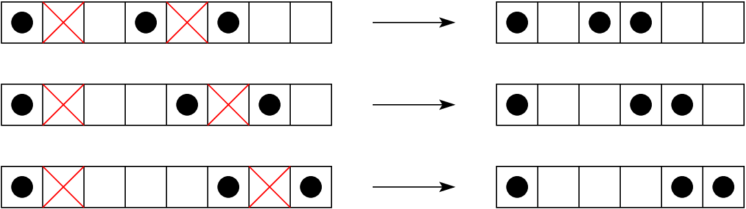
For $P$-particle excluded configurations $\ket{\mathbf{J}^{\alpha}}$ and $\ket{\mathbf{J}^{\beta}}$, the matrix element $\braket{\mathbf{J}^{\alpha}|H_{A}|\mathbf{J}^{\beta}}$ is nonzero only when $\ket{\mathbf{J}^{\alpha}}$ and $\ket{\mathbf{J}^{\beta}}$ can be obtained from one another by a single particle hopping to the left or the right. When this is so, the ordinary $P$-particle configurations $\ket{\mathbf{j}^{\alpha}}$ and $\ket{\mathbf{j}^{\beta}}$ they map to under the right-exclusion map are also related to each other by a single particle hop. Thus, we have

Since there is a one-to-one correspondence between $P$-particle configurations on an open excluded chain and $P$-particle configurations on an open ordinary chain, Eq. (10) tells us that $H_{A}$ and $H_{a}$ are identical as matrices in their respective configurational bases. We therefore conclude that the $P$-particle energy spectra of the two chains coincide, and that there is a one-to-one correspondence between the energy eigenstates, $\{\ket{\Psi}\}$ for the excluded chain, and $\{\ket{\Psi^{\prime}}\}$ for the ordinary chain. That is, if $\ket{\mathbf{J}}\mapsto\ket{\mathbf{j}}$, and $\ket{\Psi}\mapsto\ket{\Psi^{\prime}}$, then $\ket{\mathbf{J}}$ and $\ket{\mathbf{j}}$ have the same amplitudes in $\ket{\Psi}$ and $\ket{\Psi^{\prime}}$ respectively. This result has profound implications on the thermodynamics of the two chains, as well as that of the ladder model in the three limiting cases described in Sec. IV.1, because their partition functions are the same. However, for the rest of this paper, we limit ourselves to the ground states of the infinite excluded and ordinary chains, as well as those of the infinite ladder.

In this subsection, we explain how the expectation $\braket{O}$ of an observable $O$ in the ground state of the excluded chain can be computed, by relating it to the expectation $\braket{O^{\prime}}$ in the ground state of the ordinary chain, for an appropriately chosen observable $O^{\prime}$ satisfying some basic correspondence requirements that we shall outline. Specifically, we are interested in the correlations $\braket{O_{1}O_{2}}$ between two local observables $O_{1}$ and $O_{2}$ separated by a distance $r$ within the excluded-chain ground state. However, the right-exclusion map maps excluded matrix elements $\braket{\mathbf{J}^{\alpha}|O_{1}O_{2}|\mathbf{J}^{\beta}}$ to ordinary matrix elements $\braket{\mathbf{j}^{\alpha}|O^{\prime}_{1}O^{\prime}_{2}|\mathbf{j}^{\beta}}$ in which $O^{\prime}_{1}$ and $O^{\prime}_{2}$ are separated by varying separations. To deal with this problem, we develop a method of intervening-particle expansion involving a sum over conditional expectations.

To begin, let us look at the ground states

of the excluded and ordinary chains respectively. To take advantage of the equality of amplitudes, $\Psi_{0}(\mathbf{J})=\Psi^{\prime}_{0}(\mathbf{j})$ if $\ket{\mathbf{J}}\mapsto\ket{\mathbf{j}}$ under the right-exclusion map, we want $\braket{\mathbf{j}^{\alpha}|O^{\prime}|\mathbf{j}^{\beta}}$ to have a simple relation with $\braket{\mathbf{J}^{\alpha}|O|\mathbf{J}^{\beta}}$. While it is possible to pick $O^{\prime}$ such that $\braket{\mathbf{j}^{\alpha}|O^{\prime}|\mathbf{j}^{\beta}}=\braket{\mathbf{J}^{\alpha}|O|\mathbf{J}^{\beta}}$ for all $\alpha$ and $\beta$, we find that it is more convenient to pick $O^{\prime}$ such that

For example, if $O=N_{j}=C_{j}^{\dagger}C_{j}$, we can pick the corresponding observable to be $O^{\prime}=n_{j}=c_{j}^{\dagger}c_{j}$, in which case we find that

which satisfies Eq. (12) trivially. We call $O$ and $O^{\prime}$ a corresponding pair of observables, if Eq. (12) is satisfied for all $\alpha$ and $\beta$, allowing us to write the very simple relation

between their ground-state expectations.

Since we are mostly interested in correlation functions within the excluded chain ground state, let us look at expectations of the product form $\braket{O_{j}O_{j+r}}$, where $O_{j}$ acts locally about site $j$, and $O_{j+r}$ acts locally about site $j+r$. Becasue the number of particles $p$ between sites $j$ and $j+r$ varies from excluded configuration to excluded configuration, these sites get mapped by the right-exclusion map to sites on the ordinary chain with varying separations $r-p$. Therefore, to calculate the excluded chain ground-state expectation $\braket{O_{j}O_{j+r}}$ in terms of ordinary chain ground-state expectations, we first write down an intervening-particle expansion

where $\braket{O_{j}Q_{\mathbf{p}}O_{j+r}}$ are conditional expectations. Here $\mathbf{p}$ is a vector of occupation numbers within the intervening sites, and $Q_{\mathbf{p}}$ is a string of factors, each of which is either $N_{j+s}$ or $(\mathbb{1}-N_{j+s})$, $1\leq s\leq r-1$. The sum is over all possible ways to have intervening particles between $O_{j}$ and $O_{j+r}$. For each excluded term $\braket{O_{j}Q_{\mathbf{p}}O_{j+r}}$ in Eq. (15), we then write down the corresponding ordinary expectation $\braket{O^{\prime}_{j}Q^{\prime}_{\mathbf{p}^{\prime}}O^{\prime}_{j+r-p}}$, and thereafter sum over all corresponding ordinary expectations,

making use of Eq. (14). The vector $\mathbf{p}^{\prime}$ of occupation numbers is obtained from $\mathbf{p}$ using the right-exclusion map, and contains the same number $p$ of occupied intervening sites.

To illustrate how the corresponding expectations $\braket{O^{\prime}_{j}Q^{\prime}_{\mathbf{p}^{\prime}}O^{\prime}_{j+r-p}}$ can be constructed, let us write Eq. (15) out explicitly as

each of which contains intervening particles at fixed sites. We call terms in the expansion with $p$ intervening $N_{j}$’s the $p$-intervening-particle expectations. Because of nearest-neighbor exclusion, most of the terms in Eq. (17) vanish.

Next, we map each conditional excluded expectation in Eq. (17) to a corresponding conditional ordinary expectation following the simple rules given below:

1. 1.

   Nearest-neighbor exclusion. To ensure that we do not violate nearest-neighbor exclusion, we make the assignment

   $$A_{j+s}^{\dagger}A_{j+s+1}^{\dagger}=0=A_{j+s}A_{j+s+1}.$$

   (18)

   Note that this is intended not as a statement on the operator algebra, but as a mere bookkeeping device for evaluating expectations. The assignment

   $$A_{j+s}^{\dagger}N_{j+s+1}=0=N_{j+s}A_{j+s+1}$$

   (19)

   follows from Eq. (18).

2. 2.

   Right-exclusion map. The right-exclusion map described in Section II.1 is then implemented by making the substitution

   $$A_{j+s}^{\dagger}(\mathbb{1}-N_{j+s+1})\mapsto a_{j+s}^{\dagger}.$$

   (20)

   The assignment

   $$N_{j+s}(\mathbb{1}-N_{j+s+1})=n_{j+s}$$

   (21)

   follows from Eq. (20).

3. 3.

   Re-indexing. Because the right-exclusion map in Eq. (20) merges the occupied site $j+s$ and the empty site $j+s+1$ to its right, operators to the right of site $j+s+1$ must be re-indexed. The index $j+s$ on the excluded chain becomes

   $$j+s-\sum_{s^{\prime}=0}^{s-1}N_{j+s^{\prime}}$$

   (22)

   on the ordinary chain. Thus, two ending operators $r$ sites apart in the $p$-intervening-particle excluded expectation becomes $r-p$ sites apart in the corresponding $p$-intervening-particle ordinary expectation.

In the intervening-particle expansions of the two-point functions $\braket{B_{j}^{\dagger}B_{j+r}}$ and $\braket{C_{j}^{\dagger}C_{j+r}}$, the nonvanishing terms map to $p$-intervening-particle expectations of the form $\braket{b_{j}^{\dagger}\prod_{j_{p}}n_{j_{p}}\prod_{j_{h}}(\mathbb{1}-n_{j_{h}})b_{j+r-p}}$ and $\braket{c_{j}^{\dagger}\prod_{j_{p}}n_{j_{p}}\prod_{j_{h}}(\mathbb{1}-n_{j_{h}})c_{j+r-p}}$. Both can be evaluated in terms of two-point functions

of the one-dimensional Fermi sea, after invoking the Jordan-Wigner transformation (see Appendix A) for the former.

As shown in the inset of Fig. 2, the FL correlation $\braket{B_{j}^{\dagger}B_{j+r}}$ was found to consists of a simple power law part, decaying with a smaller exponent $\alpha_{0}$, and an oscillatory power law part, decaying with a larger exponent $\alpha_{1}$. Multiplying $\braket{B_{j}^{\dagger}B_{j+r}}$ by various simple powers of $r$, we find that $\sqrt{r}\braket{B_{j}^{\dagger}B_{j+r}}$ asymptotes to a constant with large $r$ (as shown in the main plot of Fig. 2), which suggests that $\alpha_{0}=\frac{1}{2}$. This is the correlation exponent predicted by Efetov and Larkin, in their study of the ordinary chain of hardcore bosons [10].

Another important result comes from the unrestricted nonlinear curve fits of $\sqrt{r}\braket{B_{j}^{\dagger}B_{j+r}}$ to the asymptotic form $A_{0}+A_{1}\,r^{-\alpha^{\prime}_{1}}\,\cos(kr+\phi_{1})$. In Fig. 3 we show a plot of the fitted wave number $k$ as a function of the density $\bar{N}$ of the excluded chain of hardcore bosons. As we can see, the fitted wave numbers fall neatly onto the straight line $k=2k_{F}=2\pi\bar{N}$, where $k_{F}=\pi\bar{N}$ is the Fermi wave number. The fact that $k_{F}$ appears naturally in the numerical correlations is expected from Luttinger’s theorem, which states that the volume of the reciprocal space bounded by the noninteracting Fermi surface is invariant quantity not affected by interactions, and applies in both Fermi and non-Fermi liquids [11, 2, 12, 13, 14, 15, 16]. From this point onwards, we restrict the wave number of the oscillatory part of the correlation functions to $k_{F}$, $2k_{F}$, or $4k_{F}$ in the nonlinear curve fits.

From the restricted nonlinear curve fits, we find that $A_{1}$ is large when $\alpha^{\prime}_{1}$ is large, and small when $\alpha^{\prime}_{1}$ is small. This suggests that neither of these parameters can be accurately determined from our nonlinear curve fits, unless we further constrain what values $\alpha^{\prime}_{1}$ can take. We also find that the quality of the nonlinear curve fit is good when $\bar{N}$ is far from $\bar{N}=\frac{1}{4}$, but deteriorates as we approach quarter filling. This suggests important physics in the FL correlation $\braket{B_{j}^{\dagger}B_{j+r}}$ near quarter filling, which cannot be adequately accounted for by an asymptotic form $A_{0}+A_{1}\,r^{-\alpha^{\prime}_{1}}\,\cos(kr+\phi_{1})$. This loss of fit also affects the phase shift $\phi_{1}$, presumably to a smaller extent, and the amplitude $A_{0}$ of the simple power law, to an even smaller extent. These two parameters are plotted as functions of the density in Fig. 4. In the limit $\bar{N}\to 0$, we have essentially a dilute gas of hardcore (otherwise noninteracting) bosons, and thus $\braket{B_{j}^{\dagger}B_{j+r}}$ should include an overall factor of $\bar{N}$. Thus we expect $A_{0}\to 0$ as $\bar{N}\to 0$. In the limit $\bar{N}\to\frac{1}{2}$, the excluded chain of hardcore bosons becomes increasingly jammed, and the relevant degrees of freedom are holes. For a dilute chain of holes, we expect $\braket{B_{j}^{\dagger}B_{j+r}}$ to be proportional to the hole density, and thus $A_{0}\to 0$ as $\bar{N}\to\frac{1}{2}$. From our numerical results alone, it is hard to tell whether $A_{0}$ reaches a maximum at $\bar{N}=\frac{1}{5}$ (corresponding to a quarter-filled, $\bar{n}=\frac{1}{4}$, ordinary chain of hardcore bosons) or $\bar{N}=\frac{1}{4}$ (quarter-filled excluded chain of hardcore bosons). It is also hard to say anything definite about the phase shift $\phi_{1}$, which might in fact be constant.

In contrast, the FL correlation $\braket{C_{j}^{\dagger}C_{j+r}}$ contains no simple power law part. A preliminary unrestricted nonlinear curve fit of this correlation to the asymptotic form $A_{1}\,r^{-\alpha_{1}}\,\cos(\pi\bar{N}r+\phi_{1})$ suggests that $\alpha_{1}\approx 1$ for all densities, i.e. may be universal $\alpha_{1}=1$ just as for noninteracting spinless fermions. However, a more careful restricted nonlinear curve fit $r\braket{C_{j}^{\dagger}C_{j+r}}=A_{1}\cos(\pi\bar{N}r+\phi_{1})$ show systematic deviations, as shown in Fig. 5, and therefore we perform an unrestricted fit to $r\braket{C_{j}^{\dagger}C_{j+r}}=A_{1}\,r^{1-\alpha_{1}}\,\cos(\pi\bar{N}r+\phi_{1})$. The fitted parameters $A_{1}$, $1-\alpha_{1}$, and $\phi_{1}$ are shown in Fig. 6.

At very low densities $\bar{N}\to 0$, our dilute chain of nearest-neighbor excluding spinless fermions will behave like noninteracting fermions, so we expect

From our curve fits, we see that in this limit, $A_{1}\to 1/\pi=0.31831\dots$, $1-\alpha_{1}\to 0$, and $\phi_{1}\to 3\pi/2$, and thus the FL correlation does indeed go to the low density limit in Eq. (24).

Also, in the half-filling limit $\bar{N}\to\frac{1}{2}$, the chain become more and more congested, making it increasingly difficult to annihilate a spinless fermion at site $j+r$, find an empty site $j$ to create a spinless fermion, without running afoul of the nearest-neighbor exclusion constraint. This tells us that $A_{1}$ must vanish as $\bar{N}\to\frac{1}{2}$, which is hinted at in Fig. 6. However, the vanishing amplitude is only half of the story in this limit, the other half being the rate at which the correlation decay with increasing separation. In fact, very close to $\bar{N}=\frac{1}{2}$, we expect the ground-state physics of the chain of rung-fermions with infinite nearest-neighbor repulsion to be describable in terms of a low density of holes. Naively, we would expect from such a low-density-of-holes argument that $\braket{C_{j}^{\dagger}C_{j+r}}$ decay as $r^{-1}$. Instead, the nonlinear curve fits at $\bar{N}_{1}\lesssim\frac{1}{2}$ tells us that $\alpha_{1}<1$.

Thinking about this nearly-half-filled limit more carefully, we realized that what we called ‘holes’ are really domain walls separating a region in which the spinless fermions sit on odd sites, from a region in which the spinless fermions sit on even sites. The FL correlation $\braket{C_{j}^{\dagger}C_{j+r}}$, which can be written as a hole-hole correlation function, then depends on how many holes there are between $j$ and $j+r$. The idea is that, in order to annihilate a hole (create a spinless fermion) at site $j+r$ and create a hole (annihilate a spinless fermion) at site $j$, we must first find a configuration with a hole at $j+r$. Such a configuration will have spinless fermions at sites $j+r-2$, $j+r-4$, …, until we encounter another hole at $j+r-2s$, and then the sequence of spinless fermions will thereafter be at sites $j+r-2s-1$, $j+r-2s-3$, …. If $r$ is even, $\braket{C_{j}^{\dagger}C_{j+r}}$ receives nonzero contributions only from those configurations with an even number of intervening holes, whereas if $r$ is odd, $\braket{C_{j}^{\dagger}C_{j+r}}$ receives nonzero contributions only from those configurations with an odd number of intervening holes. This is very similar in flavor to the intervening-particle expansion of the two-point function $\braket{b_{j}^{\dagger}b_{j+r}}$ of a chain of ordinary hardcore bosons, except that $\braket{b_{j}^{\dagger}b_{j+r}}$ receives positive contributions from configurations with an even number of intervening particles, and negative contributions from an odd number of intervening particles. Therefore, in the limit $\bar{N}\to\frac{1}{2}$, we find that the FL correlation $\braket{C_{j}^{\dagger}C_{j+r}}$ maps to a string correlation of holes. Bosonization calculations then show that this string correlation of holes decay as a power law, with correlation exponent $\alpha_{1}=\frac{1}{4}$ [17].

Important physics can also be learnt from the nonlinear curve fitting of the CDW correlations $\braket{N_{j}N_{j+r}}\equiv\braket{B_{j}^{\dagger}B_{j}B_{j+r}^{\dagger}B_{j+r}}=\braket{C_{j}^{\dagger}C_{j}C_{j+r}^{\dagger}C_{j}}$. First we tried to fit the subtracted CDW correlation to the asymptotic form $\braket{N_{j}N_{j+r}}-\braket{N_{j}}\braket{N_{j+r}}=B_{1}\,r^{-\beta_{1}}\,\cos(2\pi\bar{N}r+\theta_{1})$, but found the quality of fit deteriorates as $\bar{N}\to 0$, as shown in Fig. 7. We understand this as follows: for $\bar{N}\to 0$, the dimensionless quantity $\xi=\bar{N}r$ is small, and the poor fit indicates that $\braket{N_{j}N_{j+r}}$ contains contributions from a term that decays more rapidly than $B_{1}\,r^{-\beta_{1}}\,\cos(2\pi\bar{N}r+\theta_{1})$. If we assume that this faster decaying term is a simple power law of the form $B_{2}\,r^{-\beta_{2}}$, and fit the CDW correlation to $\braket{N_{j}N_{j+r}}=B_{1}\,r^{-\beta_{1}}\,\cos(2\pi\bar{N}r+\theta_{1})+B_{2}\,r^{-\beta_{2}}$, we found the quality of the nonlinear curve fit is improved, after dropping data points $r=2,3$ from the fit, as shown in Fig. 7. We can include the simple power law decay term in the nonlinear curve fit throughout the entire range of $\bar{N}$, but the parameters $B_{2}$ and $\beta_{2}$ cannot be reliably determined beyond $\bar{N}=\frac{1}{4}$. Therefore, the parameters $B_{1}$, $\beta_{1}$, and $\theta_{1}$ are the only parameters that can be reliably determined across the whole range of densities. From Fig. 8, we find that $\theta_{1}$ changes very little over the whole range of densities, and remains close to $\pi/16$. On the other hand, the leading correlation exponent $\beta_{1}$ appears to be density-dependent, and is very close to being

Just as for the FL correlation, we need to again think hard about the hole physics of the ground-state CDW correlation very close to half-filling. In this limit, the CDW correlation $\braket{N_{j}N_{j+r}}$ can be written in terms of the hole-density-hole-density correlation $\braket{P_{j}P_{j+r}}$, where $P_{j}=\mathbb{1}-N_{j}$ is the hole occupation number operator on site $j$. Using an argument similar to the one used for the FL correlation $\braket{C_{j}^{\dagger}C_{j+r}}$ near half-filling, we realized that if $r$ is even, $\braket{P_{j}P_{j+r}}$ receives nonzero contribution from configurations with an even number of intervening holes, whereas if $r$ is odd, $\braket{P_{j}P_{j+r}}$ receives nonzero contribution from configurations with an odd number of intervening holes. This means that our hole-density-hole-density correlation $\braket{P_{j}P_{j+r}}$ must be mapped to a string correlation of a chain of noninteracting spinless fermions. Bosonization calculations tell us that this string correlation decays as a power law with correlation exponent $\alpha=\frac{1}{2}$, consistent with the conjectured behaviour, Eq. (25), at the special value $\bar{N}=\frac{1}{2}$ [17].

In contrast to the FL and CDW correlations, the SC correlation $\braket{A_{j-2}^{\dagger}A_{j}^{\dagger}A_{j+r}A_{j+r+2}}$ on the excluded chain has a rather more complex structure. The SC correlation is always negative, and oscillations are highly suppressed, suggesting that it is the sum of a simple power law and an oscillatory power law. To improve the reliability of the nonlinear curve fits, we prescale the SC correlation by multiplying it by $r^{7/4}$. This strange exponent is chosen because it is closest to the rate at which the simple power law decay for various densities. After dropping data points for $r=2,3,4$, good fits to the asymptotic form $r^{7/4}\braket{A_{j-2}^{\dagger}A_{j}^{\dagger}A_{j+r}A_{j+r+2}}=C_{0}\,r^{7/4-\gamma_{0}}+C_{1}\,r^{7/4-\gamma_{1}}\,\cos(2\pi\bar{N}r+\chi_{1})$ were obtained. The nonlinear curve fits were improved marginally by adding a correction term of the form $C_{2}\,r^{7/4-\gamma_{2}}\,\cos(4\pi\bar{N}r+\chi_{2})$ (see Fig. 9). The fitted parameters are shown in Fig. 10 as functions of the excluded chain density $\bar{N}$.

Unlike for the FL and CDW correlations, there are no analytical bosonization calculations to help suggest values for the SC correlation exponents, so we used an ad-hoc process where we imposed trial values of the exponents, and let the nonlinear curve fitting program find the appropriate amplitudes and phase shifts. We found visually that the best fit of the numerical SC correlations appears to the mixed asymptotic form

For the ladder model described by Eq. (2), with $V\to\infty$, the ground state is determined by the two independent model parameters, $t_{\perp}/t_{\parallel}$ and $t^{\prime}/t_{\parallel}$, and the density $\bar{N}_{2}$. For fixed $\bar{N}_{2}$, the two-dimensional region in the ground-state phase diagram is bounded by three limiting cases,

1. (i)

   the paired limit $t^{\prime}\gg t_{\parallel},t_{\perp}$, which we will discuss in detail in Sec. IV.2. In this limit, we find SC correlations dominating at large distances (though, as for hardcore bosons, CDW correlations inevitably dominate at short distances). Based on our numerical studies in Sec. IV.2, the leading SC correlation exponent appears to be universal, with a value of $\gamma=\frac{1}{2}$, while the leading CDW correlation exponent $\beta$ is nonuniversal. In this limit, FL correlations are found to decay exponentially. A staggered form of long-range CDW order also appears;

2. (ii)

   the two-leg limit $t_{\perp}\ll t_{\parallel}$, $t^{\prime}=0$, which we will discuss in detail in Sec. IV.3. In this limit, the two legs of the ladder are coupled only by infinite nearest-neighbor repulsion. The dominant correlations at large distances are those of a power-law CDW, for which we find numerically to have what appears to be an universal correlation exponent of $\beta=\frac{1}{2}$. In this limit, the leading SC correlation exponent was predicted analytically to be $\gamma=2$, while FL correlations are found to decay exponentially;

3. (iii)

   the rung-fermion limit $t_{\perp}\gg t_{\parallel}$, $t^{\prime}=0$, which we will discuss in detail in Sec. IV.4. In this limit, the particles are effectively localized onto the rungs of the ladder. When the ladder is quarter-filled, a true long-range CDW emerges in the two-fold degenerate ground state. Below quarter-filling, we find numerically that the CDW power-law correlation dominate at large distances, with a leading non-universal correlation exponent $\beta=\frac{1}{2}+\frac{5}{2}\left(\frac{1}{2}-\bar{N}_{1}\right)$. The leading FL correlation exponent was also found numerically to be non-universal, with values going from $\alpha=1$ to $\alpha=\frac{1}{4}$. The SC correlation exponent, on the other hand, was found numerically to be universal, with value $\gamma=\frac{7}{4}$.

To zeroth order (i.e. without plunging into first-order perturbation theory calculations), the ground-state phase diagram can be obtained by interpolating between these three limiting cases. There will be three lines of quantum phase transitions or cross-overs, which at quarter-filling, separate the long-range CDW (LR-CDW), power-law CDW (PL-CDW), and SC phases. At quarter-filling, we expect these three lines of critical points or cross-overs to meet at a point on the phase diagram. If we have three lines of true critical points, this point would be a quantum tricritical point. We therefore end up with a ground-state phase diagram which looks like that shown in Figure 11.

In this subsection, we solve for the ground-state wave function, and calculate various ground-state correlations in the paired limit $t^{\prime}\gg t_{\parallel},t_{\perp}$. In this limit, the Hamiltonian in Eq. (2) simplifies to

In Sec. IV.2.1, we explain how pairs of spinless fermions are bound by correlated hops in this limit, and the degrees of freedom in the system become mobile bound pairs with infinite nearest-neighbor repulsion. These bound pairs come in two flavors, determined by the specific arrangement of the two bound-pair particles around a plaquette. These flavors are conserved by correlated hops if the length of the ladder is even, and hence the ladder ground state is two-fold degenerate. We then describe how these two degenerate ladder ground states can be mapped to a excluded chain of hardcore bosons, then to an ordinary chain of hardcore bosons, and finally to a chain of noninteracting spinless fermions.

In Sec. IV.2.2, we calculate the SC and CDW correlations, using the intervening-particle expansion described in Sec. II.2. We then use a restricted-probability argument in Sec. IV.2.3 to show that FL correlations decay exponentially with distance, governed by a density-dependent correlation length, in this paired limit. We find, as expected from making the absolute correlated hopping amplitude $t^{\prime}$ large, that SC correlations dominate at large distances.