Notes on Using Control Variates
for Estimation with Reversible MCMC Samplers
Abstract
A general methodology is presented for the construction and effective use of control variates for reversible MCMC samplers. The values of the coefficients of the optimal linear combination of the control variates are computed, and adaptive, consistent MCMC estimators are derived for these optimal coefficients. All methodological and asymptotic arguments are rigorously justified. Numerous MCMC simulation examples from Bayesian inference applications demonstrate that the resulting variance reduction can be quite dramatic.
Keywords — Bayesian inference, log-linear models, mixtures of Normals, probit, threshold autoregressive models, variance reduction
1 Introduction
Markov chain Monte Carlo (MCMC) methods provide the facility to draw, in an asymptotic sense, a sequence of dependent samples from a very wide class of probability measures in any dimension. This facility – together with the tremendous increase of computer power in recent years – makes MCMC perhaps the main reason for the widespread use of Bayesian statistical modeling across the entire spectrum of quantitative scientific disciplines.
This paper provides a firm methodological foundation for the construction and use of control variates for reversible MCMC samplers. Although popular in the standard Monte Carlo setting, control variates have received little attention in the MCMC literature. The proposed methodology will be shown, in many instances, to reduce the variance of the resulting estimators quite dramatically.
In the simplest Monte Carlo setting, when the goal is to compute the expected value of some function evaluated on independent and identically distributed (i.i.d.) samples , the variance of the standard ergodic averages of the can be reduced by exploiting available zero-mean statistics. If there are one or more functions – the control variates – for which it is known that the expected value of is equal to zero, then adding any linear combination, to the does not change the asymptotic mean of the corresponding ergodic averages. Moreover, if the best constant coefficients are used, then the variance of the estimates is no larger than before and often it is much smaller. The standard practice in this setting is to estimate the optimal adaptively, based on the same sequence of samples; see, e.g., Liu (2001), Givens and Hoeting (2005), Robert and Casella (2004) for details. Because of the demonstrated effectiveness of this technique, in many important areas of application – e.g., in computational finance where Monte Carlo methods are a basic tool for the approximate computation of expectations, see Glasserman (2004) – a major research effort is devoted to the construction of effective control variates in specific applied problems.
However, up to now little has been established in the way of extending the above methodology to estimators based on MCMC samples, at least in part due to the intrinsic difficulties presented by the Markovian structure. For example, Mengersen et al. (1999) comment that “control variates have been advertised early in the MCMC literature (see, e.g., Green and Han (1992)), but they are difficult to work with because the models are always different and their complexity is such that it is extremely challenging to derive a function with known expectation.” Indeed, there are two fundamental difficulties; not only is it hard to find nontrivial functions with known expectation with respect to the stationary distribution of the chain, but also, even in cases where such functions are available, there is no effective way to obtain useful estimates of the corresponding optimal coefficients . The reason why this is a fundamentally difficult problem is that the MCMC variance of ergodic averages is intrinsically an infinite-dimensional object: It cannot be written in closed form as a function of the transition kernel and the stationary distribution of the chain.
An early reference of variance reduction for Markov chain samplers is Green and Han (1992), who exploit an idea of Barone and Frigessi (1989) and construct antithetic variables that may achieve variance reduction in simple settings but they do not appear to be widely applicable. Andradòttir et al. (1993) focus on finite state space chains, they observe that optimum variance reduction can be achieved via the solution of the associated Poisson equation (see Section 2.1), and they propose numerical algorithms for its solution. Rao-Blackwellisation has been suggested by Gelfand and Smith (1990) and by Robert and Casella (2004) as a way to reduce the variance of MCMC estimators. Also, Philippe and Robert (2001) investigated the use of Riemann sums as a variance reduction tool in MCMC algorithms. An interesting as well as natural control variate that has been used, mainly as a convergence diagnostic, by Fan et al. (2006), is the score statistic. Although Philippe and Robert (2001) mention that it can be used as a control variate, its practical utility has not been investigated. Atchadé and Perron (2005) restrict attention to independent Metropolis samplers and provide an explicit formula for the construction of control variates based on adaptive estimators. Mira et al. (2003) note that a solution to the Poisson equation provides the optimum control variate and they attempt to solve it numerically. Hammer and Håkon (2008) construct control variates for general Metropolis-Hastings samplers by expanding the state space. To estimate the optimal coefficients they use the same formula that one obtains for control variates in i.i.d. Monte Carlo sampling, but such estimators are strictly suboptimal; they are briefly discussed in Section 2.3, where we also explore their efficiency.
A more relevant, for our purposes, line of work is that initiated by Henderson (1997), who observed that, for any real-valued function defined on the state space of a Markov chain , the function has zero mean with respect to the stationary distribution of the chain. Henderson (1997), like some of the other authors mentioned above, also notes that the best choice for the function would be the solution of the associated Poisson equation, and proceeds to compute approximations of this solution for specific Markov chains, with particular emphasis on models arising in stochastic network theory.
The gist of our approach is to adapt Henderson’s idea for the construction of control variates, and use them in conjunction with a new, efficiently implementable and provably optimal estimator for the coefficients for reversible chains. The ability to estimate the effectively makes these control variates practically relevant in the statistical MCMC context, and allows us to avoid having to compute analytical approximations to the solution of the underlying Poisson equation. Our estimator for is adaptive, in the sense that is based on the MCMC output, and it can be used after the sample is obtained, making its actual computation independent of the MCMC algorithm.
This methodology not only generalizes the classical method of control variates to the MCMC setting, it also offers an important advantage: Unlike the case of independent sampling where control variates need to be found in an ad hoc manner depending on the specific problem at hand, here the control variates (as well as estimates for the corresponding optimal coefficients) come for free. The only requirement for the application of this method at the post-processing stage is the availability of a function of the sampled parameters, together with its one-step conditional expectation, . As we show in numerous specific examples, these are often readily available; for example, the availability of such expectations is essentially a prerequisite for Gibbs sampling.
For any one particular application, there is, of course, a plethora of functions (and, consequently, of corresponding control variates ) that can be used, so an important consideration for the effectiveness of this methodology for variance reduction is the careful choice of these functions. This issue is addressed in detail; we provide numerous illustrative examples of estimation problems based on MCMC samplers, motivated primarily by Bayesian inference problems. These examples are chosen as representing different major classes of MCMC samplers commonly used in important applications. In each case, the ideas underlying the choice of the functions are explained, and these choices are justified either rigorously or heuristically, in connection with the theoretical development we present.
The examples we consider range from the simplest, illustrative samplers, to complex applications of Bayesian models to real data. In all cases, the resulting variance reduction is very significant and often quite large: For all the MCMC-based ergodic estimators we consider, the use of control variates gives variances at least times smaller, and often hundreds or thousands of times smaller.
Presently we focus only on cases of reversible MCMC samplers for which the one-step conditional expectations, , of one or more functions are available analytically in closed form. MCMC algorithms with this property include a vast array of samplers commonly used in practical Bayesian inference problems. In the examples presented in Sections 3 and 6 below we outline the implementation details of our methodology for a representative subset of both simple and complex models. Since our estimators for are applicable to reversible chains, we employ random-scan instead of the usual systematic-scan Gibbs or Metropolis-within-Gibbs algorithms. We also investigate the behavior of our estimators on discrete state space, random-walk Metropolis-Hastings samplers, and on Metropolis-within-Gibbs samplers. Although, strictly speaking, our theoretical development does not necessarily require that conditional expectations be analytically available, almost all of the examples presented here do have that property, primarily for the sake of convenience and of clarity of exposition. Further ongoing work by Dellaportas et al. (2008) explores ways in which this same theory can be applied to arbitrary reversible MCMC samplers, including cases where one-step conditional expectations are unavailable.
As mentioned above, Henderson (1997) takes a different path toward optimizing the use of control variates for Markov chain samplers. Considering primarily continuous-time Markov processes, an approximation for the solution to the associated Poisson equation is derived from the so-called “heavy traffic” or “fluid model” approximations of the original process. The motivation and application of this method is primarily related to examples from stochastic networks and queueing theory. Closely related approaches are presented by Henderson and Glynn (2002) and Henderson et al. (2003), where the effectiveness of network control policies of multiclass networks is evaluated via Markovian simulation tools. There, control variates are used for variance reduction, and the optimal parameters are estimated via an adaptive, stochastic gradient algorithm. General convergence properties of ergodic estimators using control variates are derived by Henderson and Simon (2004), in the case when the solution to the Poisson equation (either for the original chain or for an approximating chain) is known explicitly. Kim and Henderson (2007) introduce two related adaptive methods for tuning non-linear versions of the parameters , when using families of control variates that naturally admit a non-linear parameterization. After deriving asymptotic properties for these estimators, they present numerical examples for a simulation problem related to pricing derivative instruments in computational finance. In the case when the control variate is defined in terms of a function that can be taken as a Lyapunov function for the chain , Meyn (2006) derives precise exponential asymptotics for the performance of estimators employing such control variates.
The rest of the paper is organized as follows. Section 2.1 gives the basic definitions that will remain in effect throughout the paper, and motivates the construction of control variates in connection with the Poisson equation. Sections 2.2, 2.3 and 2.4, building on ideas of Henderson (1997), illustrate the use of naive estimators of the optimal coefficient for a single control variate, and develop the theory for two new estimators for reversible chains. In Section 3 we investigate the impact of these estimators on variance reduction in five small MCMC examples, which are representative of a larger class of Bayesian inference problems. Section 4 discusses the effect of our estimators on bias reduction, compares the two estimators and advocates the use of one of them for general purposes. These estimators are generalized in Section 5 to the case of multiple control variates. Four more complex Bayesian inference problems that are implemented via MCMC are visited in Section 6; guidelines for constructing appropriate control variates are given, and their effects on variance reduction are illustrated. Finally, we provide theoretical justifications of our asymptotic arguments in Section 7 and conclude with a short discussion of possible further extensions in Section 8.
2 Control Variates for Markov Chains
2.1 The setting
Suppose is a discrete-time Markov chain with initial state , taking values in the state space with an associated -algebra . In typical applications, will often be a (Borel measurable) subset of together the collection of all its (Borel) measurable subsets. [More precise definitions and detailed assumptions will be given in Section 7.] The distribution of is described by its transition kernel, ,
| (1) |
It is well known that in many applications where it is desirable to compute the expectation of some function with respect to some probability measure on , it turns out that, although the direct computation of is impossible or we cannot even produce samples from , we can construct an easy-to-simulate Markov chain which has as its unique invariant measure. Under appropriate conditions, the distribution of converges to , a fact which can be made precise in several ways. For example, writing for the function,
we have that, for any initial condition ,
for an appropriate class of functions . Furthermore, the rate of this convergence can be quantified by the function,
| (2) |
where is easily seen to satisfy the Poisson equation for , namely,
| (3) |
To see that, at least formally, simply apply to both sides of (2) and note that the resulting series for becomes telescoping and simplifies to .
The above results describe how the distribution of converges to . In terms of estimation, the quantities of interest are the ergodic averages,
Again, under appropriate conditions the ergodic theorem holds,
| (4) |
for an appropriate class of functions . Moreover, the rate of this convergence is quantified by an associated central limit theorem, which states that,
where , the asymptotic variance of , is given by,
Alternatively, it can be expressed in terms of the solution to Poisson’s equation as,
| (5) |
The results in equations (2) and (5) clearly indicate that it is useful to be able to compute the solution to the Poisson equation for . In general this is a highly nontrivial – or impossible – task; for one thing, it requires knowledge of the mean . The following example is one of the rare cases where explicit computations are possible.
Suppose is a discrete time version of the Ornstein-Uhlenbeck process defined by, and where is a constant in and are independent and identically distributed (i.i.d.) standard Normal random variables. Standard methods easily show that the distribution of converges to , so if we take , then, a.s., as . Moreover, the central limit theorem implies that,
where is given by (5). In order to compute the variance we need to know . As a first guess, we take and compute,
For this to be equal to , we need ; any will do. Taking, for simplicity, , yields,
Therefore, writing for random variable,
2.2 Control variates
Suppose that, for some Markov chain with transition kernel and invariant measure , we use the ergodic averages as in (4) to estimate the mean of some function under . In many applications, although the estimates converge to as , the associated asymptotic variance is large and the convergence is very slow.
In order to reduce the variance, we employ the idea of using control variates, as in the case of simple Monte Carlo with i.i.d. samples; see, for example, the standard texts Robert and Casella (2004); Liu (2001); Givens and Hoeting (2005), or the paper by Glynn and Szechtman (2002) for extensive discussions. Given a function for which we know that , define,
| (6) |
and consider the modified estimators,
We will concentrate exclusively on the the following class of functions proposed by Henderson (1997). For an arbitrary with , define,
The invariance of under and the integrability of immediately imply that . [See Section 7 for the details, complete assumptions, and full, rigorous results corresponding to this discussion.] Therefore, the ergodic theorem guarantees that the are consistent with probability one, and it is natural to seek particular choices for and so that the asymptotic variance of the modified estimators is significantly smaller that the variance of the standard ergodic averages .
Suppose, at first, that we have complete freedom in the choice of , so that we may set without loss of generality. Then we wish to make the asymptotic variance of,
as small as possible. But, in view of the Poisson equation (3), we see that the choice yields,
| (7) |
which has zero variance. Therefore, our first rule of thumb for choosing is:
Choose a control variate with .
As mentioned above, it is typically impossible to compute for realistic models in applications. But it is often possible to come up with a guess that approximates , or at least some for which heuristics indicate that it would be useful as a control variate. Once such a function is selected, we form the modified estimators with respect to the function as in (6),
The next task is to choose so that the resulting variance,
is minimized. Note that, from the definitions,
| (8) |
Therefore,
Expanding the above expression as a quadratic in , the optimal value for is determined as,
| (9) |
Note that, since , the denominator is simply . Once again, this expression depends on , so it is not immediately clear how to estimate directly from the data . We consider the issue of estimating in detail below, but first let us interpret the optimal value of . Starting from the expression,
simple calculations lead to,
so that can also be expressed as
| (10) |
leading to the optimal asymptotic variance,
| (11) |
Therefore, in order to reduce the variance, we want to have the covariance between and to be as large as possible. This leads to our second rule of thumb for selecting control variates:
Choose a control variate so that and are highly correlated.
Incidently, note that, since the denominator of (9) equals , comparing the expressions for in (9) and (11) we see that,
| (12) |
Moreover, the fact that is always nonnegative, suggests that there should be a way to rewrite the expression in the denominator of in a way which makes this nonnegativity obvious. Indeed:
Lemma 1. The asymptotic variance of the function can be expressed as,
| (13) |
Proof. Starting from the right-hand side of (13),
as claimed. The fact that is immediate upon noting that .
In view of Lemma 1, can also be expressed as,
| (14) |
2.3 A suboptimal empirical estimate of
Let be a Markov chain with transition kernel and invariant measure . In order to estimate the mean of some function under , we replace the ergodic averages of (4) by the modified estimates where the control variate for some fixed function , which, we hope, approximates the solution to the Poisson equation for , or, at least, is strongly correlated with . In order to select a “good” value for the coefficient – a value that leads to a relatively small asymptotic variance for the estimates – we first consider the following simplistic scheme.
Pretending momentarily that is a sequence of i.i.d. samples with distribution , then and the optimal coefficient choice for becomes,
which can be adaptively estimated by,
This leads us to the usual adaptive estimator for , commonly used in the case of i.i.d. samples,
To examine its performance when used on samples from a Markov chain, we consider an example.
Example 1. A simple Gibbs sampler. Let be a bivariate Normal distribution with zero mean, unit variances, and covariance . We use the systematic-scan Gibbs sampler to simulate from . Starting from arbitrary and , is generated by sampling from , and then is generated by sampling from . Continuing this way produces a Markov chain with distribution converging to .
Suppose we wish to estimate the expected value of under . Letting , the standard estimates a.s., but when is close to 1 the variance is high and the convergence very slow. In this particularly simple example, we can actually solve the Poisson equation for . Since is quadratic, we consider a candidate solution of the form . Direct calculation shows that,
and for this to be identically equal to , it suffices to take and Therefore,
From this we can compute the asymptotic variance of the estimates by substituting in (5), to obtain,
which is indeed high for
And now suppose that, as is typically the case in applications, is not available and we cannot obtain an explicit solution for . In order to create a control variate it is natural to start with itself, since we certainly expect that will be strongly correlated with . But only depends on , so, in order to take advantage of the fact that we also produce samples for , we let and define the control variate,
We will now compare the performance of three estimators: The standard estimator ; The suboptimal adaptive estimator based on the control variate defined above; and The optimal estimator based on the same control variate , but with respect to the optimal value of .
Since in this case we know both and explicitly, for the sake of comparison we compute the theoretically optimum value of appearing in (9) as,
Figure 1 shows a typical realization of the performance of all three estimators for the following parameter values: The correlation , the number of steps , the initial values are , and the optimal value of . In this experiment, the (estimated) variance of the adaptive estimator is smaller than that of the standard estimator by a factor of ; whereas the variance of the optimal estimator is smaller than that of the standard estimator by a factor of .
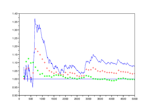
The reduction in the variance was computed from independent repetitions of the same experiment. For , we obtained different estimates , for , and the variance of was estimated by,
| (15) |
where is the average of the . The same procedure was applied to estimate the variance of and . The factors by which the variance of is larger than that of and , respectively, are shown in Table 1.
| Variance reduction factors | ||||
|---|---|---|---|---|
| Simulation steps | ||||
| Estimator | ||||
| 3.16 | 2.96 | 3.13 | 3.01 | |
| 18.28 | 16.43 | 18.52 | 16.07 | |
For different values of the number of iterations , the corresponding variance reduction factors were computed based on independent runs, and are not continuations of shorter runs. Note that the adaptive estimates were actually computed in two steps: First the value for the coefficient was computed, and then the values were calculated. In both passes, the same simulation samples were used. We emphasize that this procedure is used throughout the paper. Indeed, the fact that the estimators can be computed after the MCMC sample has been obtained is a major advantage of our methodology.
Clearly, although the adaptive estimator does offer a significant advantage over , there is a lot to be gained from obtaining more accurate estimates of the optimal coefficient . We remark that, instead of treating the samples as being i.i.d., more accurate estimates for can be obtained by approximating the expression (10) via averages over blocks. Nevertheless, extensive simulation experiments clearly indicate that the corresponding estimation gains are usually negligible, while the optimal, consistent estimation procedures for given in the following section make a very significant difference.
2.4 Optimal empirical estimates of for reversible chains
Let denote the generator of a discrete time Markov chain with transition kernel . If the chain is reversible, then is a self-adjoint linear operator on the space . This simply means that,
for any two functions . Our central result in terms of the estimation methodology is the observation that, in this case, the optimal coefficient admits a representation that does not involve the solution to Poisson’s equation :
Proposition 1. If the chain is reversible, then the optimal coefficient for the control variate can be expressed as,
| (16) |
or, alternatively,
| (17) |
Proof. Let denote the centered version of , and recall that solves Poisson’s equation for , so . Therefore, the numerator in the expression for in (9) can be expressed as,
The expressions (16) and (17) immediately suggest estimating via,
The resulting estimators, and for based on the control variate and the coefficients and , respectively, are denoted,
An alternative way for estimating adaptively, which also applies to non-reversible chains, was recently developed in Meyn (2007), based on the “temporal difference learning” algorithm. As most of the chains we will consider are reversible and this alternative method is computationally significantly more expensive than our estimates and it will not be considered further in the present discussion.
A slightly more general case of the earlier example with a bivariate Gaussian density is considered below; the random-scan Gibbs sampler is used to examine the performance of the two new estimators. We note that although the systematic-scan Gibbs sampler in general does not produce a reversible chain, the random-scan Gibbs sampler always does. Also, the back-and-forth version of the systematic-scan Gibbs sampler is reversible, see Roberts (1992).
Example 2. The bivariate Gaussian through the random-scan Gibbs sampler. Let be an arbitrary bivariate Normal distribution, where, without loss of generality, we take the expected values of both and to be zero and the variance of to be equal to one. Let and the covariance for some . Given arbitrary initial values and , the Gibbs sampler selects one of the two co-ordinates at random, and either updates by sampling from , or from . Continuing this way produces a reversible Markov chain with distribution converging to .
To estimate the expected value of under , we let and , so that,
and the control variate is, We will compare the performance of five estimators: The standard estimator ; The suboptimal adaptive estimator based on the control variate defined above; The two adaptive estimators and for the same control variate ; The optimal estimator based on the same control variate, but with respect to the optimal value of .
In Figure 2 we plot the results of all five estimators, applied to a typical execution of the Gibbs sampler with steps and initial values . The problem parameter values are and .
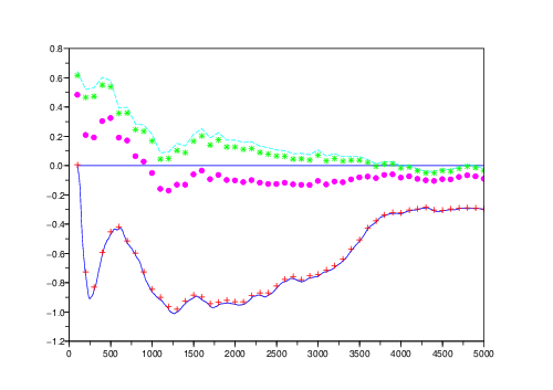
While the optimal estimator offers an obviously large advantage over the standard estimates , the improvement of the suboptimal estimator is rather insignificant. The adaptive estimators and are similarly very effective, and their performance is fairly close to that of the optimal As in Example 1, we compute the factor by which each of these methods reduces the variance of the standard estimates , using independent repetitions of the same experiment; recall equation (15) above. The results are shown in Table 2.
| Variance reduction factors | |||||
|---|---|---|---|---|---|
| Simulation steps | |||||
| Estimator | |||||
| 1.04 | 1.03 | 1.02 | 1.02 | 1.02 | |
| 2.14 | 6.25 | 6.77 | 8.26 | 7.50 | |
| 2.79 | 5.66 | 6.58 | 8.19 | 7.54 | |
| 5.23 | 9.12 | 8.20 | 8.25 | 7.53 | |
Clearly, both adaptive estimators , perform very well, and their results are reasonably close to those of the optimal estimator . A natural way to attempt to obtain an even greater improvement in terms of variance reduction would be to consider a control variate based on a of the form , for coefficients . But there is no obvious choice for the relationship between these two coefficients, and also we do not want to develop methods that are too model-specific. A generic way to address such problems is to consider two control variates , , based on the two different functions and . The corresponding methodology for such cases is developed in Section 5, where we also revisit this example.
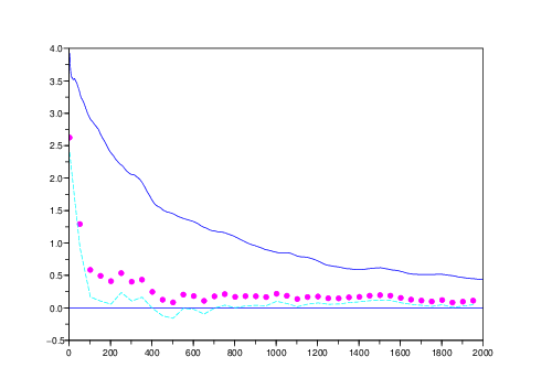
Another well-known difficulty with the standard estimates in this example (in addition to their high variance) is that they converge very slowly when the initial values of the Gibbs sampler are far from their mean. The above results are from simulations with , and we also run several examples with different initial values. In those cases we found that a lot of the time the estimators and not only reduced the variance, but also greatly improved the bias. An example with initial values and is shown in Figure 3. A more detailed discussion of this issue will be given in Section 4, where we also address the question of choosing between the two adaptive estimators, and .
3 Five Simple MCMC Examples
Below we present five examples more closely motivated by problems in statistical inference. Among the vast array of simple MCMC samplers that can be used for illustration purposes, we have chosen a set of representative examples that cover a broad class of real applications. The Gaussian-Gamma posterior in Example 3, as well as the the bivariate Gaussian density of Example 2, are representative of the large class of normal hierarchical models that are analyzed in Gelfand et al. (1990). Similarly, the Gibbs sampler of Example 4 is seen as a simplistic version of a wide class of models that include discrete variables as latent variable indicators or model indices. The discrete state space random-walk Metropolis algorithm in Example 5 is used in model search algorithms in which analytical or approximate integration of all model parameters is first performed; see for example Clyde and George (2004). A simple version of a finite-mixtures mode of Normals is explored in detail in Example 6. This this class of models has been, and still is, one of the most challenging inference problems. Finally, we illustrate our methodology in the case of a “difficult” model where Cauchy priors result in heavy-tailed posterior densities; such densities are commonly met in, for example, spatial statistics; see Dellaportas and Roberts (2003) for an illustrative example.
Example 3. A Gaussian-Gamma posterior. First we consider an example of the random-scan Gibbs sampler applied to simple Bayesian inference problem. The model is a simple two-parameter example of Gilks (1986), in which we begin with observations that are independently generated from a distribution, and we place priors and on the parameters and , respectively. [Throughout the paper, the paramatrization of the Gamma density is chosen so that it has mean .] It is straightforward that Gibbs sampling from the posterior proceeds by updating given from a Normal density with mean and variance , and given from a Gamma density with index and scale . In our simulation, we assume that and that the data vector is given by , so that the sample mean is zero. We wish to estimate the posterior mean of , so we let . Although in general this posterior mean is not computable in closed form, here the posterior marginal density of is proportional to the product of a Student’s density with mean zero (because the sample mean of is zero) and the prior density. Therefore, the resulting density is symmetric around zero, which implies that the posterior mean of is actually zero. We compare the performance of the simple empirical averages with the adaptive estimators and , based on the control variate with .
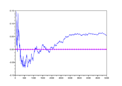
Figure 4 shows a typical random-scan Gibbs sampling run of length , with starting values . It is obvious from the plot that both adaptive estimators converge incredibly fast compared to the standard ergodic averages . The corresponding variance reduction factors, computed from repetitions of the same experiment, are shown in Table 3.
| Variance reduction factors | ||||
|---|---|---|---|---|
| Simulation steps | ||||
| Estimator | ||||
| 9403 | 341095 | 419766 | 20453186 | |
| 713 | 1880 | 5287 | 15495 | |
Given the tremendous effectiveness of the control variate with , it is natural to ask if perhaps a multiple of actually solves the Poisson equation, that is, if . Since and in the simulation experiments both and apparently converge to values very close to 2, we examine the relationship, . Substituting the expressions for and this becomes,
| (18) |
which, in our case, is indeed an equality, since the empirical mean of our sample is equal to zero. More generally, this will be an approximate equality (at least for most of the relevant values of and ), as long the empirical mean of the sample is close to zero, or if most of the mass of the posterior on is concentrated near zero. In fact, a multiple of will always solve the Poisson equation exactly, as long as the mean of the Gaussian prior on instead of zero is taken to be equal to the sample mean of .
The above discussion explains the effectiveness of the control variate with , but it also suggests that if the number of observations is small, and either: the sample mean of the observations is not close to zero; or the empirical standard deviation of is not appropriately “small” (in other words, the posterior on is not concentrated near zero); then this would not be an approximate solution to the Poisson equation, and the corresponding control variate would be much less effective. Nevertheless, even in the unlikely scenario where the observation vector is , using the same control variate as before is quite effective; see the corresponding results in Table 4.
| Variance reduction factors | ||||||
|---|---|---|---|---|---|---|
| Simulation steps | ||||||
| Estimator | ||||||
| 0.02 | 0.01 | 0.00 | 0.44 | 3.43 | 3.87 | |
| 0.37 | 4.46 | 4.17 | 8.81 | 7.88 | 6.50 | |
The reason this scenario is referred to as being “unlikely” is because the set of observations was actually obtained as an i.i.d. sample (rounded off to two decimal places) from the density; it has sample mean equal to 4.924, and sample variance . Therefore, having a prior on the mean of the observations that actually vary between 4.47 and 5.24 is an unreasonable choice. Also note that both of the potential sources of concern , above apply here. Indeed, for , the right-hand-side of (18) is , which is certainly not close to zero. Still, using the control variate with consistently yields nontrivial variance reduction factors.
Example 4. An example with a discrete variable. Next we construct a bivariate density with a discrete variable and a continuous variable , where and . The random-scan Gibbs sampler draws randomly from either or from .
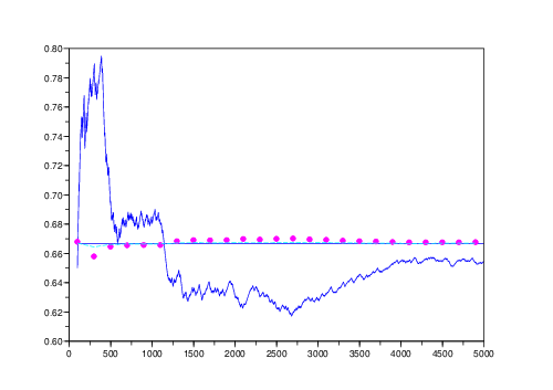
We wish to estimate the mean of , so we set and examine the performance of the ergodic averages and the two adaptive estimators and based on the control variate ; for we take, as before, . Figure 5 depicts a typical realization of the random-scan Gibbs sampler, with , , starting values , and steps. Here, the true value of is . The corresponding variance reduction factors, estimated from repetitions of the same experiment, are shown in Table 5.
| Variance reduction factors | ||||||
|---|---|---|---|---|---|---|
| Simulation steps | ||||||
| Estimator | ||||||
| 5.89 | 24.50 | 41.40 | 212.8 | 702.5 | 1721.3 | |
| 247.4 | 1286.5 | 2145.8 | 4235.4 | 12066 | 24777 | |
Like in Example 3, since the use of the control variate decreases the MCMC variance dramatically, it is natural to check if perhaps a multiple of solves the Poisson equation. Direct computation gives,
so that,
Indeed, then, is a multiple of the solution of the Poisson equation for ,
and the optimal coefficient for is,
This explains the effectiveness of this particular choice of the function . Incidently, it is somewhat remarkable that a multiple of the same function solves the Poisson equation for any choice of the parameter values .
Example 5. Random-walk Metropolis for Poisson generation. Consider the target distribution . When the mean is large, it is hard to sample from directly and, instead, we consider a random-walk Metropolis sampler, which, given , proposes a move to , where the increments are i.i.d. and or with probability each. The acceptance probability can be easily computed as,
Suppose we wish to estimate the mean of under , so let . To use a control variate with respect to some function on the integers, note that is,
so that, in particular, taking , we have,
Figure 6 shows a typical realization of the Metropolis sampler, using , with initial value , for simulation steps. The “true” mean of under is estimated to be , after 3 million Metropolis steps. The corresponding variance reduction factors, estimated from repetitions of the same experiment, are shown in Table 6.

| Variance reduction factors | ||||
|---|---|---|---|---|
| Simulation steps | ||||
| Estimator | ||||
| 0.91 | 0.32 | 0.15 | 0.20 | |
| 4.73 | 39.19 | 157.5 | 239.98 | |
Example 6. A two-parameter Gaussian mixture posterior. We examine a simple Gaussian mixture example as in Robert and Casella (2004, Example 9.2). Suppose are independent observations from the mixture ; the mixing proportion and the variance are assumed fixed and known, and priors are placed on the means . To facilitate sampling from the posterior, the model can alternatively be described in terms of latent variables , where the are independent with distribution and, conditional on and , each , and .
Conditional on and , the parameters and are independent, with,
| (19) |
respectively, where is the number of that are equal to 1, and is the number of that are equal to zero. Also, given and , the are independent, and for each ,
| (20) |
The random-scan Gibbs sampler here draws a sample from , , or from the entire vector , each chosen with probability .
We consider an example with the exact same parameter settings as in Robert and Casella (2004, Example 9.2): With , , and , we generated samples from the mixture . In order to estimate , the function is set to be . Using a control variate with the simplest choice of , yields variance reduction factors around 4, which are significantly smaller than those achieved in some of the earlier examples. For that reason, we also consider as a different candidate for the control variate . In fact, we let , and select the value of so that a multiple of is as close as possible to a solution of the Poisson equation, that is, , for some ; substituting the values of , and , and taking to be equal to the prior expectation of (namely, zero), this becomes,
| (21) |
where the are the Bernoulli parameters of the , given in (20). A reasonable goal here is to choose so as to reduce the variability of the left-hand-side as much as possible, since it is not directly related to . Ideally, this would mean taking , but since is itself random, we take to be equal to the (prior) expectation of that expression, namely, , so that the resulting function is,
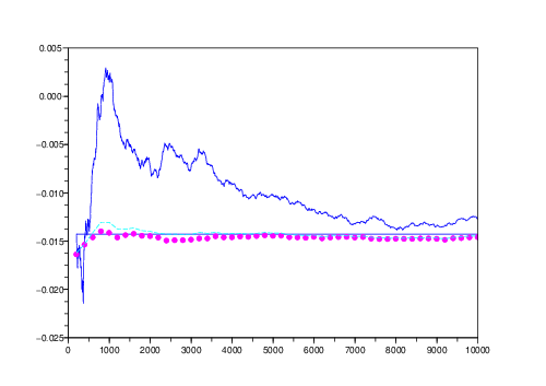
A typical realization of the estimates based on Gibbs steps is shown in Figure 7, and the corresponding variance reduction factors are displayed in Table 7. The initial values are , , and the “true” posterior mean of is estimated to be , after 10 million Gibbs steps.
| Variance reduction factors | ||||
|---|---|---|---|---|
| Simulation steps | ||||
| Estimator | ||||
| 11.76 | 15.81 | 19.02 | 22.12 | |
| 11.63 | 15.44 | 18.98 | 21.98 | |
Incidently, the above calculation suggests that the optimal value for here would be the one that also makes the right-hand-side of (21) vanish, namely, . In our simulation experiments, the estimates of produced by both and are around , which is indeed quite close.
Finally we note that models of this type often present a difficultly, in that the posterior on is bimodal. As a result, if the Gibbs sampler is initialized near the lower mode, it will never visit the neighborhood of the actual mode, at least not in any reasonable amount of time; see Robert and Casella (2004); Diebolt and Robert (1994). A more general Gaussian mixture model that at least partially addresses this issue is explored in Section 6.2.
Example 7. A Metropolis-within-Gibbs sampler. We consider an inference problem motivated by a simplified version of an example in Roberts and Rosenthal (2006). Suppose i.i.d. observations are drawn from a distribution, and place independent priors and , on the parameters , respectively. The induced full conditionals of the posterior are easily seen to satisfy,
Since the distribution is not of standard form, direct Gibbs sampling is not possible. Instead, we use a random-scan Metropolis-within-Gibbs sampler, Müller (1993); Tierney (1994), and either update from its conditional (Gibbs step), or update in a random walk-Metropolis step with a proposal, each case chosen with probability . Since both the Cauchy and the inverse Gamma distributions are heavy tailed, we naturally expect that the MCMC samples will be highly variable. Indeed, this was found to be the case in the simulation example we consider next, where the above algorithm is applied to a vector of i.i.d. observations, and with initial values and . As a result of this variability, the standard empirical averages of the values of the two parameters also converge very slowly. Since is the more variable of the two, we let and consider the problem of estimating its posterior mean. We will compare the performance of the standard empirical averages with that of the two adaptive estimators and , with the control variate defined in terms of the function . Note that, in this setting, we are restricted in our choice of functions to those which depend only on . Since is updated by an accept/reject Metropolis step, if depended on it would not be possible to compute the required one-step expectation in closed form.
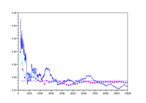
Figure 8 shows a typical realization of the results of the three estimators, for simulation steps. The “true” posterior mean of is estimated to be after 10 million simulation steps, and the corresponding variance reduction factors, estimated from repetitions of the same experiment, are shown in Table 8.
| Variance reduction factors | ||||
|---|---|---|---|---|
| Simulation steps | ||||
| Estimator | ||||
| 2.58 | 7.62 | 9.34 | 8.13 | |
| 7.89 | 7.48 | 10.46 | 8.54 | |
4 Variance, Bias and Choosing Between and
We examine how the use of the adaptive estimators estimators and can affect the estimation bias, especially in cases where the initial values of the sampler are far from the true mean of the target distribution. Also we briefly discuss the different advantages and disadvantages offered by each of these two estimators, and conclude that, generally, the preferable choice is .
4.1 Estimation bias
The primary focus of the present work is on variance reduction, more specifically, on reducing the asymptotic variance of the estimators . This variance is a “steady-state” object, in that it characterizes the long-term behavior of the averages and depends neither on the initial condition nor on the transient behavior of the chain. The bias, on the other hand, depends heavily on the initial condition, and vanishes asymptotically. Indeed, according to the expression in (2) for the solution of the Poisson equation (3),
| (22) |
which decays to zero approximately like , as .
If instead of the standard ergodic averages we use an estimator of the form based on a control variate for some function , then, replacing with in the above computation shows that the bias of is,
| (23) |
where we used the fact that , as shown in (8). Therefore, the function that minimizes (to first order) the bias of the estimates is again the solution of the Poisson equation . Of course this can also be seen directly from the definition of : As in (7), if and , then, , leading to an estimator with zero bias and zero variance.
As noted earlier, the solution to the Poisson equation cannot be computed in the vast majority of realistic examples of nontrivial Markov chains appearing in applications, if for no other reason, because it requires knowledge of the mean . Instead, a more pragmatic goal is to try and choose a “good” value for the parameter , so that the resulting estimator has significantly smaller bias than . Unlike the variance, the bias depends heavily on the initial condition , so there is no obvious choice that makes “close” to for all . In fact, for good variance reduction results we wish to have for most values near the bulk of the target distribution , whereas for the bias we need to have at the initial value of the chain, which may well be out in the tail of . Nevertheless, it may be natural to expect that taking could be a good general substitute. Although does not eliminate the bias entirely, it does bring “as close as possible” to , where “closeness” here is measured in the sense of minimizing .
In order to examine whether the choice does indeed offer an advantage in terms of the bias, we revisit Example 2 from Section 2.4, where it was observed that in some cases the adaptive estimators and did offer a significant reduction in the bias.
Example 2 revisited: Bias and MSE. As before, we use the random-scan Gibbs sampler to simulate from a bivariate Normal vector , where the expected values of both and are zero, , and their covariance with To estimate the expected value of under , we let , and take the control variate .
In Section 2.4 it was noted that, when the initial values of the sampler were relatively far from their mean (so that the samples where initially heavily biased), the adaptive estimators and not only reduced the variance, but also appeared to be correcting for the estimation bias; see Figure 3. This agrees with the intuition obtained by the discussion following the computations in (22) and (23) above. In order to get a more precise idea of the effect of the use of the adaptive estimators and on the bias and the overall estimation error, we estimate the factors by which each of these two estimators improves the bias; the variance; and the overall estimation mean-squared error (MSE). The results are shown in Tables 9 and 10; Table 9 shows simulation results for a sampler started from initial values near the true mean of the distribution, , and Table 10 shows corresponding results with initial values , .
| Example 2: | |||||
|---|---|---|---|---|---|
| Bias reduction factors | |||||
| Estimator | |||||
| 0.80 | 2.06 | 1.27 | 1.65 | 1.00 | |
| 0.83 | 1.31 | 1.02 | 1.58 | 0.75 | |
| Variance reduction factors | |||||
| 2.46 | 7.27 | 8.06 | 8.77 | 9.60 | |
| 3.51 | 6.34 | 6.62 | 8.15 | 9.33 | |
| MSE reduction factors | |||||
| 2.45 | 7.26 | 8.04 | 8.64 | 9.54 | |
| 3.46 | 6.29 | 6.59 | 8.03 | 9.29 | |
| Example 2: | |||||
|---|---|---|---|---|---|
| Bias reduction factors | |||||
| Estimator | |||||
| 1.95 | 3.66 | 4.45 | 7.97 | 7.97 | |
| 6.88 | 7.39 | 8.35 | 13.52 | 9.22 | |
| Variance reduction factors | |||||
| 1.59 | 8.04 | 9.01 | 8.66 | 9.08 | |
| 0.89 | 7.00 | 7.91 | 8.72 | 8.72 | |
| MSE reduction factors | |||||
| 2.57 | 8.34 | 9.75 | 9.11 | 9.34 | |
| 2.57 | 7.60 | 9.01 | 9.22 | 8.98 | |
The bias of the standard estimators was computed from independent repetitions of the same experiment, in a way similar to that used for the variance in the earlier examples; see the discussion in Example 1. Specifically, for , different estimates , for , were obtained from independent runs of the Gibbs sampler. Then the bias of was estimated by,
| (24) |
and the same procedure was applied to estimate the bias of and . The bias reduction factors shown in the two tables are the ratios of the corresponding (absolute values of the) bias estimates. The variance reduction factors were computed as before, and the MSE reduction factors were computed in an analogous manner.
In both cases, the results clearly show that both estimators and greatly reduce the estimation error, not only in terms of their asymptotic variance, but in terms of the bias and of the overall estimation error as well.
4.2 Choosing between the two estimators
In the simulation examples presented so far as well as in many more experiments, we observed that the overall performance of the two estimators is fairly similar. One difference is that, in cases where the initial values of the sampler were very far from the bulk of the mass of the target distribution , sometimes converged faster than and the corresponding estimator gave better results than . The reason for this discrepancy is the existence of a the time-lag in the definition of : When the initial simulation phase produces samples that approach the area near the mode of the distribution approximately monotonically, the denominator of accumulates a systematic one-sided error, and therefore takes longer to converge. But this is a transient phenomenon, and can be addressed (and often eliminated) by including a burn-in phase in the simulation.
One the other hand, we observed that the estimator was systematically more stable than , especially in the more complex MCMC scenarios involving multiple control variates. This was particularly pronounced in cases where the denominator of is near zero. There, because of the inevitable fluctuations in the estimation of this denominator, the values of fluctuated wildly between large negative and positive values, whereas the estimates were much more reliable since, by definition, the denominator of is always nonnegative.
In conclusion, we find that between and , the estimator is generally the more reliable, preferable choice. In all the examples that follow, we will restrict attention to this estimator; see also the comments at the end of Section 5.1.
5 Using Multiple Control Variates Simultaneously
5.1 Adaptive estimators with multiple control variates
Starting from the same setting of a Markov chain with transition kernel , invariant measure , and a function whose mean under is to be estimated, suppose that, instead of using a single control variate , we wish to use multiple , . One reason for such a choice is so that the optimal may potentially be approximated as a linear combination of “basis functions” , namely, .
Formally, let denote the column vector , where each is a given function , and similarly write for the column vector of control variates . For any coefficient vector , we write and consider the corresponding modified estimator for ,
[Here and throughout the paper all vectors are column vectors, and denotes the usual Euclidean inner product.] Arguing exactly as in the one-dimensional case, the asymptotic variance of can be expressed as,
| (25) |
where, stands for the vector .
To find the optimal , differentiate the quadratic with respect to each and set the derivative equal to zero, to obtain, in matrix notation,
where the matrix has entries, . Therefore,
| (26) |
as long as is invertible. Note that this expression is perfectly analogous to the one-dimensional formula for in (9). Also, in view of equation (12) from Section 2.2, the entries of can be expressed as,
This shows that has the structure of a covariance matrix and, in particular, it suggests that should be positive semidefinite. Indeed, the following lemma states that the entries of can be written in a way which makes both of these assertions obvious:
Lemma 2. Let denote the covariance matrix of the random variables
where . Then , that is, for all ,
| (27) |
Proof. Expanding the right-hand side of (27) we obtain,
and the result follows upon noting that the second and third terms above are both equal to the fourth. To see this, observe that the second term can be rewritten as,
and similarly for the third term.
Therefore, the optimal coefficient can also be expressed as,
| (28) |
Proceeding exactly as before, for a reversible chain, starting from the expressions for in (26) and (28) we obtain:
Proposition 2. If the chain is reversible, then the optimal coefficient vector for the control variates , can be expressed as,
| (29) |
or, alternatively,
| (30) |
The proof of Proposition 2 is perfectly analogous to that of Proposition 1 in the case of a single control variate.
As before, the expressions (29) and (30) suggest estimating via,
where the matrices and are defined, respectively, by,
The resulting estimators, and for based on the vector of control variates and the coefficients and , respectively, are defined analogously to the single-control-variate case as,
| (31) | |||||
| (32) |
Recall that in Section 4.2 we concluded that, for the case of a single control variate, the adaptive estimator was generally preferable to . For the same reasons, and also based on the results of extensive simulation experiments with multiple control variates, we similarly conclude that is more reliable, more stable, and generally preferable to . Therefore, in all of our subsequent examples we restrict attention to the estimator .
5.2 Examples
Here we re-examine two of the earlier examples, and illustrate how the use of multiple control variates can often provide a much greater improvement in estimation accuracy.
Example 2 revisited. Let be a zero mean, bivariate Normal distribution, with , , and for some . To estimate the expected value of under we sample from using a random-scan Gibbs sampler and set Instead of the single control variate based on , here we consider two control variates defined in terms of and , respectively. We examine the performance of the adaptive estimator , and compare it with the performance of obtained earlier by the single-control-variate estimator .
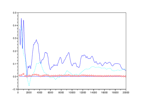
Figure 9 depicts a typical realization of the sequence of estimates of the standard ergodic averages , as well as the corresponding estimates obtained by , for simulation steps. The parameter values are and , with initial values . Table 11 shows the corresponding variance reduction factors, estimated from repetitions of the same experiment.
| Variance reduction factors | |||||
|---|---|---|---|---|---|
| Simulation steps | |||||
| Estimator | |||||
| 2.89 | 6.17 | 8.17 | 7.42 | 9.96 | |
| 4.13 | 27.91 | 122.4 | 262.5 | 445.0 | |
Clearly the estimator based on the two control variates is extremely effective, and certainly significantly better than the one based on a single control variate. As in Example 4, this effectiveness is actually explained by the fact that the exact solution of the Poisson equation in this case is of the form . Indeed, it is a simple matter to verify that,
Example 6 revisited. Recall the setting of the inference problem in Example 6 above, where, based on independent observations generated from the mixture , we wish to estimate . The mixing proportion and the variance are fixed and known, priors are placed on , and each of the binary latent variables equals if the corresponding is generated from the first component of the mixture, and otherwise. We use the random-scan Gibbs sampler, based on the full conditionals of the posterior, given in (19) and (20).
In Section 3, letting and using a control variate in terms of the function we obtained variance reduction factors around 20. The natural next step is to repeat the same experiment, this time with two control variates defined in terms of the functions and . In numerous simulation experiments we observed that, using two control variates in this case offered no apparent performance improvement. This suggests that the ratio of the coefficients of the functions and , which was earlier chosen as based on a heuristic computation, must be near-optimal. Indeed, after two million Gibbs steps, the estimated value of the optimal parameter vector for the two control variates was . The resulting optimal ratio is, as expected, quite close to .
Next we consider using four control variates, defined in terms of the functions above together with and . In this case, the corresponding variance reduction factors, estimated from repetitions of the same experiment (with initial values for the sampler , ), are 97.47, 138.39, 91.84 and 103, after and simulation steps, respectively. Compared to the earlier results (variance reduction factors around 20), these results clearly demonstrate the significant improvement in estimation accuracy due to the simultaneous use of multiple control variates.
6 Four More Complex MCMC Examples
This section illustrates our proposed methodology applied to a series of real Bayesian inference problems, providing guidelines on how functions can be chosen for the construction of effective control variates. The first example is a binary probit model, an early success of MCMC inference through data augmentation; see Albert and Chib (1993). The second example is a simple finite mixture of normals, another early application of data augmentation via Gibbs sampling; see Diebolt and Robert (1994). What makes this problem particularly interesting is the fact that, although we impose an a priori restriction on the ordering of means, the control variates methodology can still be applied after a first phase of unrestricted MCMC sampling, and after the sample has been ordered at the post-processing stage. If the objective is to estimate the means, the calculation of effective control variates is still possible, despite the fact that the resulting Markov chain has a particularly complex structure. The third example is of a Bayesian model-determination problem, in which model searching is achieved by a discrete Metropolis algorithm on the space of candidate models. Such applications have recently found tremendous interest, especially in the context of genetics (see, e.g., Bottolo and Richardson (2008)) where the model space is endowed with a multimodal discrete density. Finally, in the case of a simple log-linear model we show that, even when we are forced to consider functions that are very different from , the resulting control variates can still be very effective in terms of variance reduction.
6.1 A binary probit example
Probit models are a well-known and commonly used class of discrete regression models; see, for example, the monograph by Johnson and Albert (1999) and the references therein. Here we illustrate the use of the control variate methodology when a random-scan Gibbs sampler is used for Bayesian inference from the posterior of a binary probit model.
Specifically, we begin with an matrix of known covariates, where each is a column vector in . We also have and a vector of known binary responses , where we assume that the have,
and the unknown parameter vector is to be estimated. To facilitate sampling from the posterior of , Albert and Chib (1993) introduce independent latent random variables , where each . In other words , where is independent noise. Then the can be expressed, , so that, again, .
If we place a diffuse prior on , then and the are conditionally independent given , with,
We consider a specific example using the “statistics class” data from Johnson and Albert (1999, p. 77). In this case, for students, each is the indicator of weather student passed or failed in a statistics class. There are covariates for each student, where for all and is the th student’s SAT Math test score. We place a diffuse prior on the coefficient vector , and we consider the problem of estimating the posterior mean of . (The parameter is chosen as the more interesting of the two; the results are very similar for the case of .) To that end, we let , and we also consider a vector of control variates based on five-component function ,
For the initial condition of in the sampler we took its least-squares estimate , and for we simply drew a sample from its full conditional density as above. The choice of the function for the construction of control variates is pretty self-evident: The variables and should obviously be strongly correlated with the target variable , and the vector is included in an attempt to minimize the effect of the mean of under its full conditional.
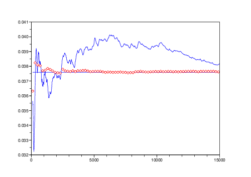
The result of a typical realization of the random-scan Gibbs sampler after iterations is shown in Figure 10. The horizontal line shows the “true” value of , the result of after 10 million Gibbs iterations. The variance reduction factors obtained by , estimated after repetitions of this experiment, are 5.08, 34.22, 53.54, 88.37 and 69.72, after , , , and iterations, respectively.
6.2 Gaussian mixtures
Mixtures of densities provide a versatile class of statistical models that have received a lot of attention from both a theoretical and a practical perspective, for many decades now. Mixtures primarily serve as a means of modelling heterogeneity for classification and discrimination, and as a way of formulating flexible models for density estimation. Although one of the fist major success stories in the MCMC community was the Bayesian implementation of the finite Gaussian mixtures problem, Tanner and Wong (1987); Diebolt and Robert (1994), there are still numerous unresolved issues in inference for finite mixtures, as discussed, for example, in the recent review paper by Marin et al. (2005). These difficulties emanate primarily from the fact that such models are often ill-posed or non-identifiable. In terms of Bayesian inference via MCMC, these issues reflect important problems in prior specifications and label switching. In particular, improper priors are hard to use and proper mixing over all posterior modes requires enforcing label-switching moves through Metropolis steps. Detailed discussions of the dangers emerging from prior specifications and identifiability constraints can be found in Marin et al. (2005); Lee et al. (2008); Jasra et al. (2005).
Here we generalize the estimation setting of Example 6 above, by employing a more realistic two-component Gaussian mixtures model as follows. Starting with data points generated from the mixture distribution , and assuming that the means, variances and mixing proportions are all unknown, we consider the problem of estimating the two means. The usual Bayesian formulation enriches that of Example 6 by introducing parameters , as follows. The data are assumed to be i.i.d. from , and we place the following priors: , the two means are independent with each , and similarly the variances are independent with each . We adopt the vague, data-dependent prior structure of Richardson and Green (1997): We set , we let equal to the empirical mean of the data , is taken to be equal to the data range, and . As before, conditional on the parameters , the latent variables are i.i.d. with and, given the entire parameter vector , the data are i.i.d. with each having distribution if , for , .
In order to estimate the mean vector we sample from the posterior via a standard random-scan Gibbs sampler, and we also introduce the a priori restriction that . In terms of the sampling itself, as noted by Stephens (1997), it is preferable to first obtain draws from the unconstrained posterior distribution and then to impose the identifiability constraint at the post-processing stage. In each iteration, the random-scan Gibbs sampler selects one of the four parameter blocks , , or , each with probability , and draws a sample from the corresponding full conditional density. These densities are all of standard form and easy to sample from; see, for example, Richardson and Green (1997). In particular, the two means are conditionally independent with each,
| (33) |
where , for . Note that the data have been generated so that the two means are very close, which results in frequent label switching throughout the MCMC run and in near-identical marginal densities of and .
We perform a post-processing relabelling of the sampled values according to the above restriction, and we denote the ordered sampled vector by . In order to estimate the posterior mean of the smaller of the two means, we let,
To reduce the variance of the estimator we consider a bivariate control variate , where the function is selected as follows. For we take the obvious choice, , so that, , the expected value of under (33), is easily seen to be,
| (34) |
where and are the means and variances of , respectively, for , under the full conditional densities in (33); see, for example, Cain (1994). Clearly this introduces a significant amount of unwanted variability in , so, in order to cancel it out, we choose to approximately cancel out the last three terms of the above expression. Since the nonlinear terms involving and are hard to handle analytically and are also bounded, and since we expect the dependence on the mean vector to be taken care of by , we focus on approximating the factor. Since will be typically small compared to and , we approximate by and by . And since we expect the influence of to be dominant over that of with respect to , a straightforward first-order Taylor expansion shows that the dominant linear term is , suggesting the choice .
To compute , we first calculate the probability that under (33),
where all four expectations above are taken under the corresponding full conditional densities, and, since the full conditional of each is a Gamma density, the expectations of , , , and , are all available in closed form. Therefore, can be computed explicitly, and,
where, again, the expectations are taken under the corresponding full conditional densities.
With this choice for , the variance reduction factors obtained by (estimated from repetitions) are 16.17, 25.36, 38.99, 44.5 and 36.16, after and simulation steps, respectively. Figure 11 shows the results of a typical simulation run. The initial values of the sampler were taken after a 1000-iteration burn-in period, and the horizontal line in the graph depicting the “true” value of the posterior mean of was obtained after 5 million Gibbs iterations.

6.3 A two-threshold autoregressive model
We revisit the monthly U.S. 3-month treasury bill rates, from January until December , previously analyzed by Dellaportas et al. (2007) using flexible volatility threshold models. The time series has points and is denoted by . Here we model these data in terms of a self-exciting threshold autoregressive model, with two regimes; it is one of the models proposed by Pfann et al. (1996), and it is defined as,
| (35) |
where , and the parameters , are the thresholds where mean or volatility regime shifts occur. Instead, we re-write the model as,
| (36) |
where characterizes the jump in between the two volatility regimes. Whereas Pfann et al. (1996) use a Gibbs sampler to estimate the parameters of the model in (35), we exploit the parameterization (36) as follows. We adopt independent improper conjugate priors for the variance, , and for the regression coefficients, . We take the prior for each of and to be a discrete uniform over the distinct values of , except the two smallest and largest values of so that identifiability is obtained; and the prior for to be an exponential density with mean one, shifted to .
Our goal is to estimate the posterior probability of the most likely model, that is, of the model corresponding to the pair of thresholds maximizing . In the above formulation, (36) can be written equivalently as, where , , is a zero-mean Gaussian vector with covariance matrix and is the design matrix with row given by (1 0 0), if , and by (0 0 1 ) otherwise. The covariance matrix of the errors, , is diagonal with if , and , otherwise. Integrating out the parameters and , the marginal likelihood of the data with known , and is,
where is the least-squares estimate of ; see, for example, O’Hagan and Forster (2004). After further performing a one-dimensional numerical integration over by numerical quadrature, we can write the marginal posterior distribution of explicitly as . Therefore, we can sample from the posterior of the thresholds by employing a discrete Metropolis-Hastings algorithm on , where the thresholds take values on the lattice of all the observed values of the rates except the two farthermost at each end. This way, we replace the -dimensional Gibbs sampler of Pfann et al. (1996) for (35), by a five-dimensional analytical integration over and , a numerical integration over , and a Metropolis-Hastings algorithm over .
Note that this algorithm is computationally less expensive, and also more reliable since Gibbs sampling across a discrete and continuous product space may encounter ‘sticky patches’ in the parameter space. The discrete Metropolis-Hastings sampler we employ is based on symmetric random walk steps, with vertical or horizontal increments of size up to ten, over the lattice of all possible values. In other words, the proposed pair given the current values is one of the forty “neighboring” pairs of , where two pairs are neighbors if they differ in exactly one co-ordinate, and by a distance of at most ten locations. Clearly, here we do not touch upon the finer issues of efficient model searching, as these would possibly require more sophisticated MCMC algorithms.
After a preliminary, exploratory simulation stage, we identified the three a posteriori most likely pairs of thresholds as being , , . To estimate the actual posterior probability of the most likely model, , we define , for , we set , and we use the control variate based on . Writing when and are neighboring pairs, can be expressed, for , as,
The resulting variance reduction factors obtained by , estimated from repetitions, are 125.16, 32.83, 36.76, 30.90 and 30.11, after and simulation steps, respectively. Figure 12 shows a typical simulation run. All MCMC chains were initiated at .

6.4 A log-linear model
We consider the table presented by Knuiman and Speed (1988), where subjects were classified according to hypertension (yes, no), obesity (low, average, high) and alcohol consumption (0, 1-2, 3-5, or drinks per day). We choose to estimate the parameters of the log-linear model with three main effects and no interactions, specified as,
where the denote the cell frequencies, modeled as Poisson variables with corresponding means , each is the th row of the design matrix , based on sum-to-zero constraints, and is the parameter vector. In Dellaportas and Forster (1999) this model was identified as having the highest posterior probability among all log-linear interaction models, under various prior specifications.
Assuming a flat prior on , standard Bayesian inference via MCMC can be performed either by a Gibbs sampler that exploits the log-concavity of full conditional densities as in Dellaportas and Smith (1993), or by a multivariate, random walk Metropolis-Hastings sampler, in which an initial maximum likelihood estimate of the covariance matrix gives guidance as to the form of the proposal density. Instead, here we use a simple random-scan Gibbs sampler, noting that a sample from the full conditional density of each can be obtained directly as the logarithm of a Gamma random variable with density,
| (37) |
In order to estimate the posterior mean of all seven components of , we set for all , and we use the same seven control variates for each , where the are defined in terms of the functions, , . The computation of is straightforward since, in view of (37), the mean of under the full conditional density of is,
The variance reduction factors obtained by after simulation steps range between 57.16 and 170.34, for different parameters . More precisely, averaging over repetitions, the variance reduction factors obtained by are in the range, 3.55–5.57, 38.2–57.69, 66.20–135.51, 57.16–170.34 and 85.41–179.11, after and simulation steps, respectively. Figure 13 shows an example of a sequence of ergodic averages for . All MCMC chains were initiated from the corresponding maximum likelihood estimates.

7 Theory
In this section we give precise conditions under which the asymptotics developed in Sections 2 and 5 are rigorously justified. The results together with their detailed assumptions are stated below and the proofs are contained in the appendix. Note that, since the first two estimators we considered, and , are special cases of the estimators and introduced in Section 5, here we concentrate on the more general estimators , .
First we recall the basic setting from Section 2. We take to be a Markov chain with values in a general measurable space equipped with a -algebra . The distribution of is described by its initial state and its transition kernel, , as in (1). The kernel , as well as any of its powers , acts linearly on functions via, .
Our first assumption on the chain is that -irreducible and aperiodic. This means that there is a -finite measure on such that, for any satisfying and any initial condition ,
Without loss of generality, is assumed to be maximal in the sense that any other such is absolutely continuous with respect to .
Our second, and stronger, assumption, is an essentially minimal ergodicity condition; cf. Meyn and Tweedie (1993): We assume that there are functions , , a “small” set , and a finite constant such that the Lyapunov drift condition (V3) holds:
| (V3) |
Recall that a set is small if there exists an integer , a and a probability measure on such that,
Under (V3), we are assured that the chain is positive recurrent, and that it possesses a unique invariant (probability) measure . Our final assumption on the chain is that the Lyapunov function in (V3) satisfies, .
These assumptions are summarized as follows:
| (A) |
Although these conditions may seem somewhat involved, their verification is generally straightforward; see the texts Meyn and Tweedie (1993); Robert and Casella (2004), as well as some of the examples developed in Roberts and Tweedie (1996); Hobert and Geyer (1998); Jarner and Hansen (2000); Fort et al. (2003); Roberts and Rosenthal (2004). In fact, it is often possible to avoid having to verify (V3) directly, by appealing to the property of geometric ergodicity, which is essentially equivalent to the requirement that (V3) holds with being a multiple of the Lyapunov function . For large classes of MCMC samplers, geometric ergodicity has been established in the above papers, among others. Moreover, geometrically ergodic chains, especially in the reversible case, have many attractive properties, as discussed, for example, by Roberts and Rosenthal (1998).
In the interest of generality, the main results of this section are stated in terms of the weaker (and essentially minimal) assumptions in (A). Some details on general strategies for their verification can be found in the references above.
Apart from conditions on the Markov chain , the asymptotic results stated earlier also require some assumptions on the function whose mean under is to be estimated, and on the (possibly vector-valued) function which is used for the control variate . These assumptions are most conveniently stated within the weighted- framework of Meyn and Tweedie (1993). Given an arbitrary function , the weighted- space is the Banach space,
With a slight abuse of notation, we say that a vector-valued function is in if for each .
Theorem 1. Suppose the chain satisfies conditions (A), and let be any sequence of random vectors in such that converge to some constant a.s., as . Then:
- (i)
[Ergodicity] The chain is positive Harris recurrent, it has a unique invariant (probability) measure , and it converges in distribution to , in that for any and ,
In fact, there exists a finite constant such that,
(38) uniformly over all initial states and all function such that .
- (ii)
[LLN] For any and any , write and . Then the ergodic averages , as well as the adaptive averages , both converge to a.s., as .
- (iii)
[Poisson Equation] If , then there exists a solution to the Poisson equation, , and is unique up to an additive constant.
- (iv)
[CLT for ] If and the variance, is nonzero, then the normalized ergodic averages converge in distribution to , as .
- (v)
[CLT for ] If , and the variances, and , are all nonzero, then the normalized adaptive averages converge in distribution to , as .
Suppose the chain satisfies conditions (A) above, and that the functions and are in . Theorem 1 states that the ergodic averages as well as the modified averages based on the vector of control variates both converge to , and both are asymptotically Normal. Next we examine the choice of the parameter vector which minimizes the limiting variance of the modified averages, and the asymptotic behavior of the estimators and for .
As in Section 5, let denote the matrix with entries, , and recall that, according to Theorem 1, there exists a solution to the Poisson equation for . The simple computation outlined in Section 5 (and justified in the proof of Theorem 2) leading to equation (26) shows that the variance is minimized by the choice,
as long as the matrix is invertible. Our next result establishes the a.s. consistency of the estimators,
where the matrices and are defined, respectively, by,
Theorem 2. Suppose that the chain is reversible and satisfies conditions (A). If the functions are both in and the matrix is nonsingular, then both the adaptive estimators for are a.s. consistent:
Recall the definitions of the two estimators and from equations (31) and (32) in Section 5. Combining the two theorems, yields the desired asymptotic properties of the two estimators:
Corollary 1. Suppose that the chain is reversible and satisfies conditions (A). If the functions are both in and the matrix is nonsingular, then the adaptive estimators and for satisfy:
- (i)
[LLN] The adaptive estimators , both converge to a.s., as .
- (ii)
[CLT] If is nonzero, then the normalized adaptive averages and converge in distribution to , as , where the variance is minimal among all estimators based on the control variate , in that
Some additional results on the long-term behavior of estimators similar to the ones considered above can be found in Meyn’s recent work in Meyn (2006) and Meyn (2007, Chapter 11).
8 Extensions
We have presented a series of small and large simulation experiments motivated by important classes of Bayesian inference problems, and we have repeatedly observed that generally straightforward choices for functions in the construction of control variates provide very effective variance reduction results. Moreover, the methodology utilizing these control variates can be implemented as an essentially black-box, post-processing algorithm.
The theory presented is applicable to any reversible Markov chain. Our focus here has been primarily on cases of samplers for which we can find some functions such that the one-step conditional expectations required for the computation of are available in closed form. These are readily available in all conjugate Gibbs and discrete Metropolis algorithms, as well as in most Markovian models for stochastic networks; see Meyn (2007) and the references therein.
Most of our experiments were performed using random-scan Gibbs samplers, in order to maintain reversibility; this is not necessarily a restrictive choice, since the convergence properties of random-scan algorithms are comparable to those of systematic-scan samplers; see Roberts and Sahu (1997). Moreover, any implementation technique that can facilitate or speed up the MCMC convergence (such as blocking schemes, transformations, other reversible chains, and so on), can be used, as long as reversibility is maintained.
There are many other Gibbs sampling algorithms in which full conditional density expectations are analytically available and, therefore, our proposed methodology is immediately applicable. Apart from the natural extensions of the examples in Section 3, we emphasize that conjugate Gibbs sampling is the key ingredient in Bayesian inference for dynamic linear models, see Reis et al. (2006); slice Gibbs auxiliary variables applications, see Damien et al. (1999); Dirichlet processes, see MacEachern and Muller (1998); and spatial regression models, see Gamermanan et al. (2003).
Metropolis-Hastings algorithms were used in Example 5 and in the two-threshold autoregressive model in Section 6.3. In both cases, the samplers operate on a discrete state space, making it possible to compute directly in closed form. It may be worth emphasizing that for any discrete Metropolis-Hastings sampler where the number of possible proposed moves is not prohibitively large, the function can be easily analytically obtained for any choice of .
In closing, we note that the main obstacle in the immediate applicability of our methodology is the presence of the accept/reject probability in Metropolis-Hastings steps with continuous proposals. The ways in which this methodology can be applied in such cases are explored in ongoing work that investigates this issue in detail, and which will be reported in Dellaportas et al. (2008).
Acknowledgments
We are grateful to Sean Meyn and Zoi Tsourti for many interesting conversations related to this work.
Appendix: Proofs of Theorems 1 and 2
Proof of Theorem 1. Since any small set is petite, Meyn and Tweedie (1993, Section 5.5.2), the -norm ergodic theorem of Meyn and Tweedie (1993) implies that is positive recurrent with a unique invariant measure such that (38) holds, and Meyn and Tweedie (1993, Theorem 11.3.4) proves the Harris property, giving (i).
From Meyn and Tweedie (1993, Theorem 14.0.1) we have that, under (V3), . Since is in , is finite, and since Jensen’s inequality guarantees that is finite. The invariance of then implies that ; therefore, Meyn and Tweedie (1993, Theorem 17.0.1) shows that and a.s. as , and since by assumption, also converges to a.s., proving (ii).
The existence of a solution to the Poisson equation in (iii) follows from Meyn and Tweedie (1993, Theorem 17.4.2), and its uniqueness from Meyn and Tweedie (1993, Theorem 17.4.1). The CLT in (iv) is a consequence of Meyn and Tweedie (1993, Theorem 17.4.4).
Finally, since , the functions and are in too, so and exist for each . As in (iv), the scaled averages and converge in distribution to and , respectively, for each , where the variances and are as in (iii). Writing and , we can express,
Each of the terms in the second sum on the right-hand-side above converges to zero in probability, since and converges to a Normal distribution and a.s. Therefore, the sum converges to zero in probability, and the CLT in (v) follows from (iv).
Note that the assumption in the theorem is not necessary, since the case is trivial in view of Kontoyiannis and Meyn (2003, Proposition 2.4), which implies that, then, in probability, as .
Proof of Theorem 2. We begin by justifying the computations in Section 5. Define , where exists by Theorem 1. Since solves the Poisson equation for , it is easy to check that solves the Poisson equation for . Substituting this in the above expression for yields (25). To see that all the functions in (25) are indeed integrable recall that and note that, since is nonnegative, (V3) implies that , hence is finite since is finite by assumption. Therefore, since , and are both in , and Hölder’s inequality implies that is finite. Finally, Jensen’s inequality implies that and are also in , so that . And, for the same reasons, all the functions appearing in the computations leading to the results of Lemma 2 and Proposition 2 are also integrable.
The expression for the optimal in (26) is simply the solution for the minimum of the quadratic in (25). Again, note that and are all in so is well-defined.
The consistency proofs follow from repeated applications of the ergodic theorems established in Theorem 1. First note that, since and as remarked above, the product is -integrable, and by Jensen’s inequality so is any product of the form . Therefore, the ergodic theorem of Meyn and Tweedie (1993, Theorem 17.0.1) implies that a.s. Similarly, the functions , , , and are all -integrable, so that the same ergodic theorem implies that indeed converges to a.s., as .
To establish the corresponding result for , it suffices to show that a.s., and to that end we consider the bivariate chain on the state space . Since is -irreducible and aperiodic, is -irreducible and aperiodic with respect to the bivariate measure . Given functions a small set and a constant so that (V3) holds, it is immediate that (V3) also holds for with respect to the functions , , the small set , and the same . The unique invariant measure of is then , and is finite. Therefore, assumptions (A) hold for and, for each pair we can invoke the ergodic theorem Meyn and Tweedie (1993, Theorem 17.0.1) for the -integrable function,
to obtain that, indeed, a.s.
Proof of Corollary 1. The ergodic theorems in (i) are immediate consequences of Theorem 1 (ii) combined with Theorem 2. The computation in Section 5 which shows that in (26) indeed minimizes (justified in the proof of Theorem 2) shows that Finally, the assumption that is nonsingular combined with Lemma 2, imply that all the variances must be nonzero. Therefore, Theorem 2 combined with the central limit theorems in parts (iv) and (v) of Theorem 1, prove part (ii) of the Corollary.
References
- Albert and Chib (1993) Albert, J. and S. Chib (1993). Bayesian analysis of binary and polychotomous response data. J. Amer. Statist. Assoc. 88(422), 669–679.
- Andradòttir et al. (1993) Andradòttir, S., D. Heyman, and T. Ott (1993). Variance reduction through smoothing and control variates for Markov Chain simulations. ACM Transactions on Modeling and Computer Simulation 3, 167–189.
- Atchadé and Perron (2005) Atchadé, Y. F. and F. Perron (2005). Improving on the independent Metropolis-Hastings algorithm. Statistica Sinica 15, 3–18.
- Barone and Frigessi (1989) Barone, P. and A. Frigessi (1989). Improving stochastic relaxation for Gaussian random fields. Probability in the Engineering and Informational sciences 4, 369–389.
- Bottolo and Richardson (2008) Bottolo, L. and S. Richardson (2008). Evolutionary stochastic search. Preprint.
- Cain (1994) Cain, M. (1994). The moment-generating function of the minimum of bivariate normal random variables. The American Statistician 48, 124–125.
- Clyde and George (2004) Clyde, M. and E. I. George (2004). Model uncertainty. Statist. Sci 19, 81–94.
- Damien et al. (1999) Damien, P., J. Wakefield, and S. Walker (1999). Gibbs sampling for Bayesian non-conjugate and hierarchical models by using auxiliary variables. Journal of the Royal Statistical Society. Series B (Statistical Methodology) 61, 331–344.
- Dellaportas et al. (2007) Dellaportas, P., D. Denison, and C. Holmes (2007). Flexible threshold models for modelling interest rate volatility. Econometric reviews 26, 419–437.
- Dellaportas and Forster (1999) Dellaportas, P. and J. J. Forster (1999). Markov chain Monte Carlo model determination for hierarchical and graphical log-linear models. Biometrika 86, 615–633.
- Dellaportas et al. (2008) Dellaportas, P., I. Kontoyiannis, S. Meyn, and Z. Tsourti (2008). Manuscript in preparation.
- Dellaportas and Roberts (2003) Dellaportas, P. and G. Roberts (2003). An introduction to MCMC, Volume Spatial Statistics and Computational methods,, pp. 1–42. Springer-Verlag, NY. J. Møller.
- Dellaportas and Smith (1993) Dellaportas, P. and A. F. M. Smith (1993). Bayesian inference for generalised linear and proportional hazards models via Gibbs sampling. Applied Statistics 42, 443–459.
- Diebolt and Robert (1994) Diebolt, J. and C. Robert (1994). Estimation of finite mixture distributions through Bayesian sampling. J. Roy. Statist. Soc. Ser. B 56(2), 363–375.
- Fan et al. (2006) Fan, Y., S. Brooks, and A. Gelman (2006). Output assessment for Monte Carlo simulations via the score statistic. Journal of Computational and Graphical Statistics 15, 178–206.
- Fort et al. (2003) Fort, G., E. Moulines, G. Roberts, and J. Rosenthal (2003). On the geometric ergodicity of hybrid samplers. J. Appl. Probab. 40(1), 123–146.
- Gamermanan et al. (2003) Gamermanan, D., A. R. Moreirab, and H. Rue (2003). Space-varying regression models: specifications and simulation. Computational Statistics and data analysis 42, 513–533.
- Gelfand et al. (1990) Gelfand, A. E., S. E. Hills, A. Racine-Poon, and A. F. M. Smith (1990). Illustration of Bayesian inference in normal data models using Gibbs sampling. Journal of the American Statistical Association 85(412), 972–985.
- Gelfand and Smith (1990) Gelfand, A. E. and A. F. M. Smith (1990). Sampling-based approaches to calculating marginal densities. Journal of the American Statistical Association 85, 398–409.
- Gilks (1986) Gilks, W. (1986). Full conditional distributions. In Markov Chain Monte Carlo in Practice (Gilks, W.R., Richardson, S. and Spiegelhalter, D., Edts.), pp. 75–88. London: Chapman and Hall.
- Givens and Hoeting (2005) Givens, G. and J. Hoeting (2005). Computational Statistics. Hoboken, NJ: John Wiley & Sons.
- Glasserman (2004) Glasserman, P. (2004). Monte Carlo Methods in Financial Engineering. New York: Springer-Verlag.
- Glynn and Szechtman (2002) Glynn, P. and R. Szechtman (2002). Some new perspectives on the method of control variates. In Monte Carlo and quasi-Monte Carlo methods, 2000 (Hong Kong), pp. 27–49. Berlin: Springer.
- Green and Han (1992) Green, P. and X. Han (1992). Metropolis methods, Gaussian proposals, and antithetic variables, Volume 74, Lecture Notes in Statistics, Stochastic Methods and Algorithms in Image Analysis, pp. 142–164. Spinger Verlag, Berlin. Eds: P. Barone, A. Frigessi and M. Piccioni.
- Hammer and Håkon (2008) Hammer, H. and Håkon (2008). Control variates for the Metropolis-Hastings algorithm. Scandinavian Journal of Statistics 35, 400–414.
- Henderson (1997) Henderson, S. (1997). Variance Reduction Via an Approximating Markov Process. Ph. D. thesis, Department of Operations Research, Stanford University, Stanford, CA.
- Henderson and Glynn (2002) Henderson, S. and P. Glynn (2002). Approximating martingales for variance reduction in Markov process simulation. Math. Oper. Res. 27(2), 253–271.
- Henderson et al. (2003) Henderson, S., S. Meyn, and V. Tadić (2003). Performance evaluation and policy selection in multiclass networks. Discrete Event Dyn. Syst. 13(1-2), 149–189. Special issue on learning, optimization and decision making.
- Henderson and Simon (2004) Henderson, S. and B. Simon (2004). Adaptive simulation using perfect control variates. J. Appl. Probab. 41(3), 859–876.
- Hobert and Geyer (1998) Hobert, J. and C. Geyer (1998). Geometric ergodicity of Gibbs and block Gibbs samplers for a hierarchical random effects model. J. Multivariate Anal. 67(2), 414–430.
- Jarner and Hansen (2000) Jarner, S. and E. Hansen (2000). Geometric ergodicity of Metropolis algorithms. Stochastic Process. Appl. 85(2), 341–361.
- Jasra et al. (2005) Jasra, A., C. Holmes, and D. Stephens (2005). Markov chain Monte Carlo methods and the label switching problem in Bayesian mixture modelling. Statistical Science 20, 50–67.
- Johnson and Albert (1999) Johnson, V. and J. Albert (1999). Ordinal Data Modeling. New York: Springer-Verlag.
- Kim and Henderson (2007) Kim, S. and S. Henderson (2007). Adaptive control variates for finite-horizon simulation. Math. Oper. Res. 32(3), 508–527.
- Knuiman and Speed (1988) Knuiman, M. and T. P. Speed (1988). Incorporating prior information into the analysis of contingency tables. Biometrics 44, 1061–1071.
- Kontoyiannis and Meyn (2003) Kontoyiannis, I. and S. Meyn (2003). Spectral theory and limit theorems for geometrically ergodic Markov processes. Ann. Appl. Probab. 13, 304–362.
- Lee et al. (2008) Lee, K., J.-M. Marin, K. Mengersen, and C. Robert (2008). Bayesian Inference on Mixtures of Distributions, Volume Proceedings of the Platinum Jubilee of the Indian Statistical Institute (to appear). Elsevier, NY. D. Dey and C.R. Rao.
- Liu (2001) Liu, J. (2001). Monte Carlo Strategies in Scientific Computing. New York: Springer-Verlag.
- MacEachern and Muller (1998) MacEachern, S. N. and P. Muller (1998). Estimating mixture of Dirichlet process models. Journal of Computational and Graphical Statistics 7, 223–238.
- Marin et al. (2005) Marin, J.-M., K. Mengersen, and C. Robert (2005). Bayesian modelling and inference on mixtures of distributions, Volume Handbook of Statistics: Volume 25. Elsevier, NY. D. Dey and C.R. Rao.
- Mengersen et al. (1999) Mengersen, K. L., C. P. Robert, and C. Guihenneuc-Jouyaux (1999). MCMC convergence diagnostics: A reviewww. In A. P. D. J. M. Bernardo, J. O. Berger and A. F. M. Smith (Eds.), Bayesian Statistics 6, pp. 415–440. Oxford University Press, UK.
- Meyn (2006) Meyn, S. (2006). Large deviation asymptotics and control variates for simulating large functions. Ann. Appl. Probab. 16(1), 310–339.
- Meyn (2007) Meyn, S. (2007). Control Techniques for Complex Networks. Cambridge University Press.
- Meyn and Tweedie (1993) Meyn, S. and R. Tweedie (1993). Markov Chains and Stochastic Stability. London: Springer-Verlag.
- Mira et al. (2003) Mira, A., P. Tenconi, and D. Bressanini (2003). Variance reduction for MCMC. Technical report 2003/29, Universitá degli Studi dell’ Insubria, Italy.
- Müller (1993) Müller, P. (1993). Alternatives to the Gibbs sampling scheme. Technical report, Institute of Statistics and Decision Sciences, Duke University.
- O’Hagan and Forster (2004) O’Hagan, A. and J. Forster (2004). Bayesian Inference. Arnold, London.
- Pfann et al. (1996) Pfann, G., S. P.C., and R. Tschernig (1996). Nonlinear interest rate dynamics and implications for the term structure. Journal of Econometrics 74, 149–176.
- Philippe and Robert (2001) Philippe, A. and C. Robert (2001). Riemann sums for MCMC estimation and convergence monitoring. Statistics and Computing 11, 103–115.
- Reis et al. (2006) Reis, E. A., E. Salazar, and D. Gamerman (2006). Comparison of sampling schemes for dynamic linear models. International Statistics Review 74, 203–214.
- Richardson and Green (1997) Richardson, S. and P. J. Green (1997). On Bayesian analysis of mixtures with an unknown number of components (with discussion). Journal of the Royal Statistical Society, Series B 59, 731–792.
- Robert and Casella (2004) Robert, C. and G. Casella (2004). Monte Carlo Statistical Methods (Second ed.). New York: Springer-Verlag.
- Roberts (1992) Roberts, G. (1992). Convergence diagnostics of the Gibbs sampler. In J. M. Bernardo, J. Berger, A. Dawid, and A. Smith (Eds.), Bayesian Statistics 4, pp. 775–782. Oxford University Press, UK.
- Roberts and Rosenthal (1998) Roberts, G. and J. Rosenthal (1998). Markov-chain Monte Carlo: some practical implications of theoretical results. Canad. J. Statist. 26(1), 5–31. With discussion by Hemant Ishwaran and Neal Madras and a rejoinder by the authors.
- Roberts and Rosenthal (2004) Roberts, G. and J. Rosenthal (2004). General state space Markov chains and MCMC algorithms. Probab. Surv. 1, 20–71 (electronic).
- Roberts and Rosenthal (2006) Roberts, G. and J. Rosenthal (2006). Examples of adaptive MCMC. Preprint. [Available online at: probability.ca/jeff/].
- Roberts and Tweedie (1996) Roberts, G. and R. Tweedie (1996). Geometric convergence and central limit theorems for multidimensional Hastings and Metropolis algorithms. Biometrika 83(1), 95–110.
- Roberts and Sahu (1997) Roberts, G. O. and S. K. Sahu (1997). Updating schemes, correlation structure, blocking and parameterisation for the Gibbs sampler. Journal of the Royal Statistical Society, Series B 59, 291–397.
- Stephens (1997) Stephens, M. (1997). Bayesian Methods for Mixtures of Normal Distributions. Ph. D. thesis, University of Oxford, UK.
- Tanner and Wong (1987) Tanner, M. A. and W. H. Wong (1987). The calculation of posterior distributions by data augmentation. Journal of the American Statistical Association 82, 528–540.
- Tierney (1994) Tierney, L. (1994). Markov chains for exploring posterior distributions. Ann. Statist. 22(4), 1701–1762. With discussion.