Systematics of High Temperature Perturbation Theory:
The Two-Loop Electron Self-Energy in QED

The systematics of the usual loop expansion in powers of the weak coupling $e^{2}=1/137\ll 1$ is well understood in quantum electrodynamics (QED), in perturbation theory about the vacuum state. However, when one considers extreme states of matter at high temperatures or densities, straightforward perturbation theory is of little use, even in a weakly coupled gauge theory like QED. At very high temperatures ($T\gg m_{e}$) one signal of the failure of the usual loop expansion is the appearance of infrared singularities of the form $(eT/\omega)^{2\ell-2}$, at $\ell$ loop order, where $\omega$ is a characteristic frequency, such as that of an external line in a self-energy diagram. The appearance of such infrared singularities implies that higher order terms in the perturbative series in $e^{2}$ are unsuppressed for low energies or momentum scales, and hence the usual perturbative loop expansion fails for $\omega\lesssim eT$.

The singular infrared behavior of perturbation theory at finite temperature can be seen already at the one-loop level. The leading order one-loop singularities arise from the ultraviolet or hard region of the momentum integral, whose power law growth is cut off only by the Bose-Einstein or Fermi-Dirac thermal distribution, so that the loop momentum becomes of order of the temperature $T$. These leading contributions in the high temperature expansion of one-loop self-energies and vertices are the hard thermal loops (HTL’s) [1], studied extensively in the 1990’s in both QED and QCD (see [2, 3, 4, 5] for reviews). It was found that the leading order (LO) HTL self-energies and proper vertices enjoy some remarkable properties [6, 7, 8], among which is that they obey the same Ward identities as those of the exact theory. This enabled Braaten and Pisarski to propose an HTL resummation program [6, 8], in which the LO HTL propagators and vertices are used instead of the bare ones in any diagram in which the loop integration momentum becomes soft ($\sim eT\ll T$). This resummation algorithm was successfully applied to a number of problems, chief among them the first determination of the damping rate of gluons at rest in the high temperature QCD plasma, which is finite and free of any gauge ambiguities [9].

The Ward identities obeyed by the lowest order HTL self-energies and vertices, and the success of HTL resummation in producing gauge invariant physical quantities suggests it should be possible to restructure the perturbative loop expansion of gauge theories at high temperatures or densities in a systematic way. To do so, however, requires a more complete understanding of the infrared singularities of the subleading terms in the high temperature expansion at higher loops. The subleading or next-to-leading order (NLO) terms in the high temperature expansion of the one-loop level fermion self-energy have been computed [10, 11], but there have been only a few partial calculations of various quantities in different kinematic limits at two-loop order [12, 13, 14, 15, 16]. As a consequence, both the nature of the subleading infrared singularities of perturbation theory which HTL resummation includes and those which it does not include, and the general systematics of the reordering of the loop expansion at high temperatures beyond HTL’s, if it exists, has remained relatively unexplored.

The promising beginning of HTL resummation of infrared singularities, and the possibility of extending its success to higher orders in a systematic way is especially interesting in gauge theories. More than just a formal question about the nature of perturbation theory at high temperatures, the lack of systematic expansion methods that can capture both collective behavior and infrared physics in hot or dense matter, and also preserve gauge invariance and the UV renormalization structure of the underlying microscopic theory is a serious obstacle to physical applications in processes from the early universe to heavy-ion collisions, both in and out of equilibrium.

Motivated by these considerations, we present in this paper a calculation of the two-loop electron self-energy $\Sigma$ in high temperature QED. Our approach is simply to calculate the two-loop self-energy in the high temperature limit, systematically extracting the leading terms at high $T$, without making any assumptions about the relative importance or unimportance of different contributions or momentum ranges, and without assuming a priori how they should be resummed. Once these leading terms in the high temperature expansion of the two-loop self-energy are known, they may be compared then with the known NLO terms of the one-loop self-energy [10, 11]. By explicit calculation we shall find that the leading terms in the high temperature expansion of the two-loop self-energy are of the same size, or even larger than the NLO terms of the one-loop $\Sigma_{1}$ when evaluated on the fermion mass shell. This is a direct demonstration of the need to take two and higher loops into account in order to obtain the full NLO result.

Dissecting the explicit two-loop self-energy calculation also allows for a more complete understanding of the relative importance of different momentum ranges in the loop integrations. It is already well known that the LO HTL result at one-loop order results from the strictly hard region of the loop integration where $p\sim T$. The NLO terms of the one-loop $\Sigma$ arise from the region of the loop momentum integral which is parametrically less than $T$. For the case of the imaginary part of $\Sigma$, the relevant momentum scale is $p\sim eT\ll T$, while the real part of the self-energy receives contributions form the entire range of loop momentum $0\leq p\lesssim T$, and give rise to $\ln(T/\omega)$ weak dependence upon the temperature. Although momenta up to $T$ do play a role in the real parts, unlike the purely hard contributions which grow as a power of $T$, logarithms are a signal of sensitivity to the low momentum, infrared region of the loop integration as well. Following the convention in the field [1, 6], we term all such contributions where internal momenta of order $eT$ or less play an important role, soft loop integrals. We shall see that the leading order terms at two loops which are comparable to the NLO terms at one loop all come from momentum integrations where one of the loops is hard, while the other is soft, in the sense just described. Thus these comparable terms coming from one- and two-loop diagrams have in common that they arise from exactly one soft internal momentum loop.

An additional signal of the need for a reordering of perturbation theory comes from the gauge dependence of the one-loop self-energy, even when evaluated on the fermion mass shell. In the LO HTL limit, i.e. when the loop momentum is hard, the one-loop electron dispersion relation is independent of the gauge fixing parameter $\xi$. However at NLO in the high temperature expansion coming from the soft region of the loop momentum integral, the one-loop dispersion relation becomes dependent upon $\xi$ [10, 11]. This is sufficient proof that the NLO one loop calculation is incomplete and physically meaningless by itself, and a systematic resummation method to obtain gauge invariant results for physical quantities such as the fermion damping rate at order $e^{2}T$ is necessary. Our calculation will show that this gauge dependence is not cured at two-loops, and a full resummation of higher loops is necessary in order to arrive at the full NLO gauge invariant decay rate of an on-shell fermion in the plasma of order $e^{2}T$.

When higher numbers of loops are considered, we encounter a new phenomenon not present at one loop. At two-loop order in addition to gauge parameter dependence of the on-shell dispersion relation, we encounter uncanceled true infrared and/or collinear divergences, not regulated even at finite values of the soft external energy $\omega$, or momentum ${\bf q}$. In particular, a linear infrared divergence appears in the bubble diagram Fig. 2 of the two-loop fermion self-energy, arising from the double photon massless propagator pole in this diagram. Quite apart from dependence upon the gauge parameter $\xi$, the appearance of such unregulated divergences from massless, unscreened photons is itself also sufficient evidence for the breakdown of the loop expansion at high temperatures, and the need for a resummation of diagrams with still larger numbers of loops.

In order to regulate the divergences in the two-loop fermion self-energy, we introduce a photon mass $M$ in the evaluation of the bubble diagram of Fig. 2. In the usual perturbative expansion, the formal limit $M\rightarrow 0$ should be taken. Since this limit does not exist at two-loop order, we may anticipate the result that after HTL resummation of the photon self-energy the photon acquires a non-zero Debye screening mass of order $eT$. Taking $M\sim eT$ allows us to characterize the order of all the two-loop contributions to $\Sigma$, and compare finite contributions from different loop orders in a meaningful way. In other words, when the formal photon regulator mass is replaced by the physical Debye screening mass, by a partial resummation of the photon propagator for soft momenta, there are neither infrared nor collinear divergences in the two-loop dressed self-energy, and all NLO contributions to the fermion self-energy are estimated correctly in powers of $e$. The photon mass $M$ thus plays a dual role in our considerations, first as a regulator of infrared divergences in bare loop diagrams, and second, as a parameter whose finite value of order $eT$ after resummation of higher loop diagrams enables us to estimate the finite magnitude of resummed amplitudes.

Both the gauge parameter dependence and the explicit infrared divergences as $M\rightarrow 0$ in the bare loop expansion can be cured only by systematically including the contributions from higher numbers of loops $\ell>2$, despite the fact that these contain additional explicit powers of the coupling. This HTL improved resummation leads finally to the complete order $e^{2}T$ corrections to the fermion dispersion relation in the plasma for both its real and imaginary parts, compared to the LO result for the fermion thermal mass, $eT/\sqrt{8}$ which is purely real. Thus the reordering of perturbation theory in the plasma is decidedly non-analytic in $\alpha=e^{2}/4\pi$.

The structure of the explicit two-loop calculation of $\Sigma$ shows that the leading contributions at high temperatures arise entirely from momentum integrals which factorize into one momentum integral which is hard ($p\sim T$), and a second one which is soft (in the sense defined above). Overlapping two-loop momentum integrals which violate this hard-soft pattern can be shown explicitly to be suppressed by additional powers of $e$, thus justifying their neglect, in ${\cal O}(e^{2}T)$ calculation of the self-energy and damping rate. In particular, the detailed analysis of the two-loop self-energy shows that there are no contributions at this order coming from both loops hard, which naive power counting would apparently allow [8, 3]. That such hard-hard contributions from two-loop diagrams at this order in $e^{2}T$ are completely absent is in accordance with the an earlier result by Schulz for the two-loop gluon polarization in QCD at next to leading order [14]. A fact apparently not widely recognized is that the contribution at two-loop order of only hard-soft integrals to terms of order $e^{2}T$ in the fermion self-energy and the complete absence of hard-hard contributions is exactly what is required by the HTL resummation program, when HTL propagators and vertices are re-expanded in primitive bare loops of perturbation theory, a point which we elaborate in some detail in Sec. V. Thus one result of our detailed evaluation of the two-loop self-energy is a refinement of naive power counting rules, and a clarification of the hard-soft factorization structure of the high temperature expansion of perturbation theory, which underpins resummation of one-loop diagrams with HTL dressed propagators and vertices.

The factorization pattern should be expected to continue at $\ell>2$ loops as well, namely all the order $e^{2}T$ corrections to the fermion dispersion relation should arise from $\ell-1$ hard loops inside only one soft loop. This HTL reordering of the ordinary loop expansion is necessary to collect all the infrared sensitive terms of relative order $(eT/\omega)^{2\ell-2}$ from $\ell$ loops, which make equally important contributions to the fermion dispersion relation and damping rate, when $\omega\sim eT$. When all these subleading contributions are summed over all $\ell$ loops by the HTL resummation of propagators and vertices in an HTL dressed one-loop diagram, the gauge parameter dependence at subleading $e^{2}T$ order is eliminated. The curing of both the infrared divergences, and the gauge parameter dependence of the ordinary bare loop expansion by the same resummation in HTL propagators and vertices, when calculating damping rates and plasma frequencies, represents an important check on its physical consistency [9, 17, 18, 14, 19, 20, 21].

The technical evaluation of the two-loop diagrams in the imaginary time formalism [3, 5] is facilitated considerably by using Gaudin’s method [22, 23], which we review in Appendix A. This very efficient method of performing the frequency sums makes calculations of diagrams involving many finite temperature propagators feasible. The Gaudin method also makes the hard-soft factorization pattern at two-loops more evident, and makes feasible the analysis of dressed and/or even higher loop diagrams, at least for the purpose of extracting their leading order behavior in the high temperature limit.

The outline of the paper is as follows. In Section II we review the one-loop finite temperature electron self-energy, including both the LO HTL and NLO terms, and the latter’s dependence upon the gauge fixing parameter $\xi$. In Section III we present the basic calculation of the three diagrams of two different topologies in the two-loop electron self-energy by the Gaudin method in the Feynman gauge, introducing the photon mass regulator for the most infrared sensitive bubble diagram. In Section IV we present the detailed analysis of the two-loop integrals obtained in Section III, for a fermion at rest ${\bf q}=0$. We show that the leading contributions in the high temperature expansion of the two-loop diagrams of both topologies come from one loop hard, the other soft, thus demonstrating explicitly that there are no hard-hard contributions, and the soft-soft contributions are subleading at this order. In Section V we compare our results with the insertions of effective HTL self-energies and vertices in the one-loop $\Sigma$, explicitly verifying the equivalence of these insertions for both the real and imaginary parts to order $e^{2}T$, which is necessary for the HTL resummation program to work. In Section VI we study the gauge parameter dependence of the two-loopself-energy, and show that it does not cancel even on shell, in neither its real or imaginary parts. Section VII contains a summary of the main results for the two-loop self-energy to order $e^{2}T$, concluding with a discussion of the lessons for a systematic reorganization of the loop expansion in high temperature gauge theories to higher orders.

We begin by setting our conventions and reviewing the existing leading order (LO) [3, 24] and NLO [10, 11] calculations of the one-loop QED electron finite temperature self-energy,

represented in Fig. 1. For the purposes of this paper, we use the Feynman rule conventions of [25] wherein the tree-level electron-photon vertex is $-ie\gamma_{\mu}.$ In (1) the tree-level fermion propagator is given by

with $\mbox{\,/\penalty\hskip-6.19995pt$K$}=\gamma^{\mu}K_{\mu}=k_{0}\gamma_{0}-{\bf k}\cdot{\bm{\gamma}}$. The tree-level photon propagator in the one-parameter family of covariant $\xi$-gauges is

We employ the somewhat redundant notation of $\tilde{D}(K)$ and $D(K)$ for the same function of $K^{2}$ in order to distinguish propagators with fermionic Matsubara frequencies from those with bosonic Matsubara frequencies in the imaginary time formalism of finite temperature field theory [3, 5]. Thus, in imaginary time where the generic four-momentum becomes $K^{\mu}=(i\omega_{n},{\bf k})$,

For evaluation of loop integrals such as that in (1) we use the convention

Moreover, our conventions are such that the electron and photon proper self-energies, $\Sigma$ and $\Pi_{\mu\nu}$, contribute to the full inverse propagators in the form

for the electron and photon respectively. The sign convention for $\Sigma$ here is the opposite of that of [11].

It will also be convenient to work with the spectral representation of the propagators, which is given by

where

Here $\rho(k_{0},{\bf k})$ is the spectral function of a free massless boson,

and $\varepsilon(k_{0})=\theta(k_{0})-\theta(-k_{0})$ is the sign function. Accordingly, the spectral representation of $\Delta(i\omega_{n},{\bf k})$ is

and similarly for $\tilde{\Delta}(i\omega_{n},{\bf k})$, with the only difference that in this latter case $\omega_{n}$ is fermionic.

In this section we compute the two-loop electron self-energy in the Feynman gauge $\xi=1$, perform the Matsubara sums in the imaginary time formalism by Gaudin’s method, and reduce the expressions to integrals over two spatial loop momenta ${\bf k}$ and ${\bf p}$, for general external electron energy and momentum $(i\nu_{q},{\bf q})$. The leading terms in the high temperature expansion arise from only those terms with two statistical factors, $n_{B}$ or $n_{F}$. The analysis of the integrals, the explicit extraction of their leading high temperature, most infrared sensitive terms, and the analytic continuation to real electron energies $i\nu_{q}\rightarrow\omega+i0^{+}$ for ${\bf q}=0$ electrons at rest in the plasma are performed in the next section.

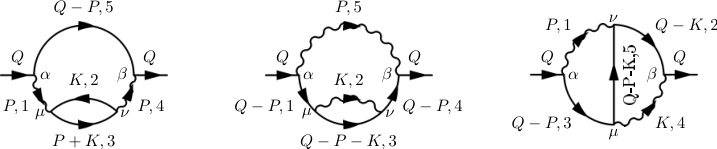
At two-loops the electron self-energy is composed of the three diagrams pictured in Fig. 2, which we call the bubble (B) diagram, the rainbow (R) diagram, and the crossed photon (C) diagram. The corresponding contributions to $\Sigma$ will be denoted by $\Sigma_{\textrm{\tiny B}}$, $\Sigma_{\textrm{\tiny R}}$ and $\Sigma_{\textrm{\tiny C}}$ respectively.

An earlier partial calculation of the two-loop electron self-energy at finite temperatures has been given the literature in Ref. [12]. The authors of this work were interested in the ultraviolet renormalizability of QED and electron mass renormalization at finite temperatures. For that reason they used real time Feynman propagators (rather than the appropriate causal real time Schwinger-Keldysh formalism), and did not calculate the imaginary parts of any of the two-loop diagrams. They also did not calculate the contribution of the bubble diagram (B), which turns out to give the dominant contribution to the real part at leading order in the high temperature expansion, in which we are interested.

The calculation of such multi-loop diagrams in the imaginary time formalism is greatly facilitated by Gaudin’s method for performing the Matsubara sums [22]. Since each of the two-loop self-energy diagrams contains five finite temperature propagators, finding the appropriate partial fraction identity analogous to (12) for disentangling the two independent Matsubara frequencies is already quite non-trivial. Gaudin’s method for doing this involves a graphical decomposition of each original two-loop Feynman diagram in $\Sigma$ into a sum of tree diagrams, each containing three propagators, and the complement of the tree containing the other two propagators which carry the two independent Matsubara frequencies. This graphical decomposition is illustrated in Fig. 3, for the case of the bubble (B) self-energy diagram. Calculations in scalar field theory using Gaudin’s method were presented in [23] on a two-loop diagram having the topology of diagram (C). Diagrams of type (R) or (B) were outside the interest of the authors of [23] because, having a self-energy insertion on an internal line, they are not in the class of two-particle irreducible (2PI) diagrams. The method works equally well on diagrams of all topologies. However, since two fermion propagators (diagram R) or two photon propagators (diagram B) have the same four-momentum, the two diagrams suffer from a double pole problem (in any method). In Gaudin’s method this problem manifest itself in two different ways, as one sees from the Gaudin tree graphs of Fig. 3. The first way is illustrated by the first four graphs, where one encounters the product of a spectral function corresponding to a line which acquires a statistical factor and a Matsubara propagator with the same four-momentum, that is $\delta(p_{0}^{2}-{\bf p}^{2})/({\bf p}^{2}-p_{0}^{2})$. The second way in which the double pole problem arises is found in the last three Gaudin tree graphs, where one encounters the product of two Matsubara propagators sharing the same 4-momentum. In both cases the expressions can be regularized by a massive regulator, which effectively defines ill-defined double pole quantities by the replacements

References

• References
• [1] R. D. Pisarski, Phys. Rev. Lett. 63, 1129 (1989).
• [2] M. H. Thoma, Applications of High Temperature Field Theory to Heavy Ion Collisions, in Quark-gluon plasma 2, edited by R. C. Hwa, World Scientific: Singapore (1995).
• [3] M. Le Bellac, Thermal Field Theory, Cambridge University Press:Cambridge (1996).
• [4] J.-P. Blaizot and E. Iancu, Phys. Rept. 359, 355 (2002).
• [5] J. I. Kapusta and Ch. Gale, Finite-Temperature Field Theory: Principles and Applications, 2nd Edition, Cambridge University Press: Cambridge (2006).
• [6] E. Braaten and R. D. Pisarski, Phys. Rev. Lett. 64, 1338 (1990).
• [7] J. Frenkel and J. C. Taylor, Nucl. Phys. B334, 199 (1990).
• [8] E. Braaten and R. D. Pisarski, Nucl. Phys. B337, 569 (1990).
• [9] E. Braaten and R. D. Pisarski, Phys. Rev. D 42, 2156 (1990).
• [10] I. Mitra, Phys. Rev. D 62, 045023 (2000).
• [11] S.-Y. Wang, Phys. Rev. D 70, 065011 (2004).
• [12] M. Qader, S. S. Masood and K. Ahmed, Phys. Rev. D 46, 5633 (1992).
• [13] T. Altherr, E. Petitgirard and T. del Rio Gaztelurrutia, Phys. Rev. D 47, 703 (1993).
• [14] H. Schulz, Nucl. Phys. B413, 353 (1994).
• [15] A. Majumder and C. Gale , Phys. Rev. C 65, 055203 (2002).
• [16] M. E. Carrington and E. Mottola, Nucl. Phys. A785, 142 (2007).
• [17] R. Kobes, G. Kunstatter and K. Mak, Phys. Rev. D 45, 4632 (1992).
• [18] E. Braaten and R. D. Pisarski, Phys. Rev. D 46, 1829 (1992).
• [19] F. Flechsig and H. Schulz, Phys. Lett. B349, 504 (1995).
• [20] M. E. Carrington, Phys. Rev. D 75, 045019 (2007).
• [21] M. E. Carrington, A. Gynther and D. Pickering, Phys. Rev. D 78, 045018 (2008).
• [22] M. Gaudin, Nuov. Cim. 38, 844 (1965).
• [23] J.-P. Blaizot and U. Reinosa, Nucl. Phys. A764, 393 (2006).
• [24] A. Peshier, K. Schertler and M. H. Thoma, Annals Phys. 266, 162 (1998).
• [25] M. E. Peskin and D. V. Schroeder, An Introduction to Quantum Field Theory, Westview Press: New York (1995).
• [26] H. A. Weldon, Phys. Rev. D 28, 2007 (1983).
• [27] V. V. Klimov, Sov. J. Nucl. Phys. 33, 934 (1981).
• [28] H. A. Weldon, Phys. Rev. D 26, 1394 (1982).
• [29] J.-P. Blaizot and E. Iancu, Phys. Rev. D 55, 973 (1997).
• [30] R. Baier, B. Pire and D. Schiff, Phys. Rev. D 38, 2814 (1988).
• [31] G. Gatoff and J. Kapusta, Phys. Rev. D 41, 611 (1990).
• [32] P. Aurenche, F. Gelis, R. Kobes, and E. Petitgirard, Z. Phys. C 75, 315 (1997).
• [33] H. Zaraket, [hep-ph/9810246], in Proceedings of the 5th Thermal Field Theory Workshop, Regensburg, 1998, edited by U. Heinz.
• [34] P. Aurenche, F. Gelis, and H. Zaraket, JHEP 0207, 063 (2002).
• [35] M. H. Thoma and C. T. Traxler, Phys. Lett. B 378, 233 (1996).
• [36] A. Abada and K. Bouakaz, JHEP 0601, 161 (2006).
• [37] R. D. Pisarski, Phys. Rev. D 47, 5589 (1993).
• [38] U. Kraemmer, A. K. Rebhan and H. Schulz, Ann. Phys. N. Y. 238, 286 (1995); A. K. Rebhan, hep-ph/960841.
• [39] P. Aurenche, F. Gelis, G. D. Moore, and H. Zaraket, JHEP 0212, 006 (2002).
• [40] S. Jeon, Phys. Rev. D 52, 3591 (1995); S. Jeon and L. G. Yaffe, Phys. Rev. D 53, 5799 (1996).
• [41] J.-S. Gagnon and S. Jeon, Phys. Rev. D 75, 025014 (2007); ibid. 76, 105019 (2007).
• [42] L. Dolan and R. Jackiw, Phys. Rev. D 9, 3320 (1974).