A Measurement of Primordial Non-Gaussianity Using WMAP 5-Year Temperature Skewness Power Spectrum
Abstract
We constrain the primordial non-Gaussianity parameter of the local model using the skewness power spectrum associated with the two-to-one cumulant correlator of cosmic microwave background temperature anisotropies. This bispectrum-related power spectrum was constructed after weighting the temperature map with the appropriate window functions to form an estimator that probes the multipolar dependence of the underlying bispectrum associated with the primordial non-Gaussianity. We also estimate a separate skewness power spectrum sensitive more strongly to unresolved point sources. When compared to previous attempts at measuring the primordial non-Gaussianity with WMAP data, our estimators have the main advantage that we do not collapse information to a single number. When model fitting the two-to-one skewness power spectrum we make use of bispectra generated by the primordial non-Gaussianity, radio point sources, and lensing-secondary correlation. We analyze Q, V and W-band WMAP 5-year data using the KQ75 mask out to . Using V and W-band data and marginalizing over model parameters related to point sources and lensing-secondary bispectrum, our overall and preferred constraint on is at the 68% confidence level ( at 95 confidence). We find no evidence for a non-zero value of even marginally at the 1 level.
pacs
98.70.Vc, 98.80.-k, 98.80.Bp, 98.80.EsI Introduction
The inflationary paradigm has deservedly become a cornerstone of modern cosmology [1, 2, 3, 6, 4, 5]. Inflation solves the flatness, horizon and the monopole problems of the standard Big-Bang cosmology. Furthermore, inflation is the prevailing paradigm related to the origin of density perturbations that gave rise to the large-scale structure we see today. It posits that a nearly exponential expansion stretched space in the first moments of the early universe and promoted microscopic quantum fluctuations to perturbations on cosmological scales today [7, 11, 9, 8, 10]. Inflation makes detailed predictions for key statistical features of these fluctuations. These predictions have now begun to be tested by a range of cosmological observations, including cosmic microwave background (CMB) temperature anisotropy and polarization.
Recent measurements of the CMB with a variety of ground, sub-orbital, and space-based experiments have provided some of the most stringent tests of inflation (e.g., [12, 13]). Specifically among the generic predictions of inflation, recent CMB measurements with the temperature anisotropy power spectrum and polarization have established (1) a nearly flat geometry, (2) a nearly scale-invariant spectrum at large angular scales, (3) adiabatic fluctuations, and (4) super-horizon flucuations through the temperature-polarization cross spectrum. One major prediction of inflation yet to be verified is the stochastic background of primordial gravitational waves [14, 6, 15]. While strong limits are expected from Planck [16], a detection of the gravitational wave background is the main focus of a next-generation space-based CMB experiment [17, 18, 19, 20].
Some other tests of inflation involve the probability distribution function and isotropy of the density perturbations generated by inflation. In the standard slow-roll inflationary model the inflaton, the hypothesized scalar field or particle responsible for inflation, fluctuates with a minimal amount of self interactions. In fact, such a small amount of self interactions ensures that the fluctuations are nearly Gaussian, and that any non-Gaussianity produced would be too small for detection [21, 25, 22, 23, 24]. Non-Gaussianity therefore would be a measure of either interactions of the inflaton [26, 27] or any non-linearities [28, 29], and a detection of non-Gaussianity would indicate a violation of slow-roll inflation.
In this spirit, models of non slow-roll inflation or alternatives to inflation have been proposed to generate large, measurable non-Gaussianities. The curvaton mechanism produces curvature perturbations associated with the fluctuations of a light scalar field whose energy density is zero [30]. The inhomogeneous reheating scenario can produce non-Gaussianity through modulated reheating during the reheating stage [31]. Using multiple inflaton fields that are allowed to interact, those interactions can be used to source non-Gaussianity [32]. Lastly, warm inflation [33], ghost inflation [34] and string theory inspired D-cceleration [35] and Dirac-Born-Infeld (DBI) inflation [36] models also give rise to a large non-Gaussianity (see review in Ref. [37]).
To connect with observable measurements, the associated non-Gaussianity of the CMB can be described in terms of the second-order correction to the curvature perturbations in position space with
| (1) |
where the non-Gaussianity parameter describes the amplitude of the second-order correction. This form was first suggested by Salopek & Bond [28, 38] to describe the non-Gaussianity in primordial perturbations from inflation and has been the subject of experimental constraints using a variety of CMB and large-scale structure data in recent years.
Instead of constraints on the non-Gaussianity parameter in the position space, recent studies make use of the bispectrum involving a three-point correlation function in Fourier or multipole space. The configuration dependence of the bispectrum with lengths that form a triangle in Fourier space can be used to separate various mechanisms for non-Gaussianities, depending on the effectiveness of of the estimator used. To summarize the status of the non-Gaussianity measurements, an analysis with WMAP 3-year data first suggested a hint of a non-Gaussianity in the local model with (95% CL), far above the value of expected in simple, single field, slow-roll inflation models [39]. The WMAP team’s preferred measurement of non-Gaussianity parameter in 5-year V and W-band data is (95% CL) [12]. The most recent constraint on comes from studying the WMAP 5-year data with an optimal estimator leading to (95% CL) [40]. At the 68% confidence level, with a value of , there is still some marginal evidence for a non-zero value of the non-Gaussianity parameter. If such a result were to continue to hold with Planck, which increases the precision of measurement by a factor of 3 to 4, then our simple inflationary picture would need to be revised to include a more complex model.
In this paper, we will pursue a new measurement of the primordial non-Gaussianity parameter with a new estimator that preserves some angular dependence of the bispectrum. On the contrary, the estimators employed by most CMB non-Gaussianity studies, including those by the WAMP team [12], involves a measurement that compresses all information of the bispectrum to a single number called the cross-skewness computed with two weighted maps. Such a drastic compression limits the ability to study the angular dependence of the non-Gaussian signal and to separate any confusing foregrounds from the primordial non-Gaussianity. In addition to Galactic foregrounds, non-Gaussianity measurements could also be contaminated by unresolved point sources, mainly radio and dusty galaxies, and Sunyaev-Zel’dovich (SZ) clusters, among others [41]. Given the increase in size of CMB data, especially with Planck, it is also necessary to develop accurate measurement techniques to extract that are unbiased.
Our estimator for non-Gaussianity uses a weighted version of the squared temperature-temperature angular power spectrum [42, 43], which we refer to as the skewness power spectrum. This power spectrum extracts information from the bispectrum as a function of the multipole of one triangle length in the harmonic space, while summing all configurations given by the other two side lengths. The difference in spatial dependence based on how the maps are weighted provides ways to separate primordial non-Gaussianity from that of the foregrounds. Here, we account for both point source and lensing bispectra with latter resulting from the correlation of the lensing potential with secondary anisotropies [44, 45].
To summarize our main results, after marginalizing over the normalizations of point source and lensing-secondary bispectra, with the combination of V and W-band maps we are able to constrain at the 68% confidence level or at the confidence level. We find that is never incompatible with zero at confidence when is estimated in independent bins of width 200 between . We find a significant contribution from unresolved point sources, but failed to detect the lensing-secondary cross-correlations using the two statistics we considered here.
In section §II we review the background theory and in §III we review the estimator used and our simulation procedure to compute the uncertainties. In §IV we discuss our methods for analyzing and simulating data. In section §V we discuss our results. In section §VI we conclude with a summary of our results.
II Theory
To begin, we define multipole moments of the temperature map through
| (2) |
The angular power spectrum and bispectrum are defined in the usual way such that
| (3) | |||||
Here the quantity in parentheses is the Wigner-3 symbol. The orthonormality relation for Wigner-3 symbol implies
The angular bispectrum, , contains all the information available from the three-point correlation function. For example, the skewness, the pseudo-collapsed three-point function of Ref. [46] and the equilateral configuration statistic of Ref. [47] can all be expressed as linear combinations of the bispectrum terms (see Ref. [29] for explicit expressions and Ref. [48] for an expression relating skewness in terms of the bispectrum).

II.1 Primordial Non-Gaussianity
Here we focus on the local form of the primordial non-Gaussianity. Using the second order correction to the curvature perturbations in equation (1) and following the derivation in Ref. [38], we write the angular bispectrum of temperature anisotropies as
where
| (11) |
and is the comoving radial coordinate.
The two functions in are given by
| (12) | |||||
| (13) |
Here, is the primordial power spectrum of Bardeen’s curvature perturbations, and is the radiation transfer function that gives the angular power spectrum as . In Fig. 1, we show four example cases of and . We generate them using a modified version of the CMBFAST code [49] and for our fiducial cosmological parameter values, consistent with WMAP 5-year best-fit model, as summarized in Table I.
| Parameter | Value |
|---|---|
| 0.02273 | |
| 0.1099 | |
| 0.963 | |
| 0.087 | |
| for Q | |
| for V | |
| for W | |
| 0.718 |
II.2 Unresolved Point Sources
In addition to the primordial bispectrum, we also account for the non-Gaussianity generated by unresolved radio point sources. If the sources are Poisson distributed, the bispectrum takes a simple from [38] with
| (14) |
where
| (15) |
where is the number counts of sources and maps flux density to thermodynamic temperature with with . This conversion can be simplified to . When model fitting to data, we will ignore the exact number counts of the unresolved sources and parameterize the uncertainty with an overall normalization
| (16) |
where the index is for the three bands from WMAP (Q, V, and W) we use here.
Here, we only account for the shot-noise contribution from point sources, similar to the analysis of non-Gaussianity measurements by the WMAP team. It is likely that unresolved point sources are clustered on the sky, though existing WMAP data with measurements at the two-point function level only lead to an upper limit on the clustering amplitude of point sources [50]. In future, especially for non-Gaussianity measurement with Planck, it may be necessary to include the bispectrum generated by clustered point sources.
II.3 CMB Lensing-Secondary Correlation
The gravitational lensing effect of the CMB also generates a bispectrum through correlations of the lensing potential with secondary anisotropies that are generated at late times [45, 44].
To understand this signal, we note that the lensed temperature fluctuation in a given direction is the sum of the primary fluctuation in a different direction plus the secondary anisotropy
| (17) | |||||
or
| (18) | |||||
Utilizing the definition of the bispectrum in Eq. (II), we obtain
| (22) | |||||
where the extra five permutations are with respect to the ordering of .
Integrating by parts and simplifying further following leads to a bispectrum of the form:
When calculating the CMB lensing potential-secondary anisotropy cross-correlation we will include both the integrated Sachs-Wolfe (ISW) and the Sunyaev-Zel’dovich (SZ) effects, with the latter modeled using the halo approach [51, 52, 53]. We will take the sum of the two effects such that . The cross-correlation between lensing potential and ISW is calculated in the standard way [54, 55] for the fiducial CDM cosmological model, using only the linear theory potential. For the lensing-SZ correlation, the linear halo model takes into account the SZ profile obtained analytically in Ref. [56] combined with the halo mass function similar to calculations of the SZ angular power spectrum. When model fitting the data, we will parameterize the overall uncertainty with a parameter for each of the WMAP bands such that .
While lensing modification to CMB bispectrum alone is not expected to make a significant correction to the non-Gaussianity measurement, analytical calculations of the lensing effect on the CMB bispectrum suggest that the lensing-secondary correlation will be the main contamination to a reliable measurement of the primordial non-Gaussianity parameter [41, 57, 58, 59]. This includes the lensing-ISW effect since SZ can be “cleaned out” in multi-frequency data such as those expected from Planck [48, 60]. It is due to this reason that we include the lensing-secondary correlation here.


III Estimators of
We will now motivate a new estimator for measuring . For this we introduce the squared temperature-temperature angular power spectrum and discuss its use as a probe of the angular bispectrum. We motivate a new estimator by revising the original form in Ref. [42].
Through the expansion of the temperature
| (27) |
we can write
| (28) |
We emphasize here that denotes the multipole moments of the temperature squared map and not the square of the multipole moments of the temperature map.
We can now construct the angular power spectrum of squared temperature and temperature as
| (29) |
After some tedious, but straightforward algebra we can write the relation between the bispectrum of the temperature field and the angular power spectrum of squared temperature and temperature as
| (30) | |||||
Here, we have made use of the relation
| (34) |
As is clear sums up all triangle configurations of the bispectrum at each of the side length of the triangle in multipolar space.
If a priori known that certain triangular configurations contribute to the bispectrum significantly one can compute this sum by appropriately weighting the multipole coefficients. This is essentially what can be achieved with the introduction of an appropriate weight or a window function in equation (28). Though the analytical expression for the two-to-one angular power spectrum involves a sum over the two sides of the angular bispectrum, the experimental measurement is straightforward: one construct the power spectrum by squaring the temperature field, in real space, and using the Fourier transforms of squared temperature values and the temperature field, with any weighting as necessary.
This simple form of the skewness power spectrum has already been used by Szapudi & Chen [61] to constrain (1) with WMAP 3-year data. The form of the skewness power spectrum as written exactly in equation (III) is not useful for a primordial non-Gaussianity measurement. We describe how to filter data for a measurement of primordial non-Gaussinity below.
III.1 Skewness Estimator
To obtain a more useful form, it is useful to review the form of the skewness statistic employed by the WMAP team, which is originating from Ref. [62]. The skewness statistic makes use of two set of maps of the CMB sky as a function of the radial distance :
| (35) | |||||
| (36) |
where
| (37) | |||||
| (38) |
Here where are the frequency dependent beam transfer functions and is the power spectrum from associated simulated noise maps. We discuss both these quantities later.
In and maps weights are such that they are are constructed from the theoretical CMB power spectrum under the assumed cosmological model, the experimental beam , and the primordial non-Gaussianity projection functions and where and are defined in equations (12) and (13).
The WMAP team’s estimator [62] uses an integration in the radial coordinate to obtain the skewness of the product of the and maps
| (39) |
In practice this skewness is corrected by an additional linear term that corrects approximately the effects of partial sky coverage associated with the mask and non-uniform noise. This term is computed by combining observed map with simulated maps that are Monte-Carlo averaged (see Appendix A of Ref. [12]).
As is clear from above involves a complete compression of data to a single number. While in principle different sources of non-Gaussianities contribute to with a single number alone it is impossible to separate out the primordial value from the non-Gaussianities generated by secondary anisotropies and other foregrounds. To some extent the separation is aided by a different set of maps that are weighted differently than the case of and maps.
A map optimized for the non-Gaussianity of the form generated by shot-noise from point sources is the map:
| (40) |
where
| (41) |
Similar to , one can also compute a skewness associated with E maps by taking . WMAP team used the latter to constrain the normalization of the point source Poisson term with .

III.2 Revised Skewness Power Spectrum
In order to revise the previously discussed skewness power spectrum, instead of simply integrating over the and maps, we extract the multipole moments of the map and the product maps
| (42) |
These two multipole moments then allow us to write the new skewness power spectrum appropriately weighted in the same manner as the previous skewness estimator:
| (43) | |||||
To see how probes the primordial bispectrum, we can write the multipole moments of the squared B map as
| (44) | |||||
where are the beam times the observed multipole moments . Note that the observed multipole moments relate to theory moments via another beam factor.
Similarly, the multipole moments of the product map is
| (49) | |||||
The power spectrum is simply then
| (55) | |||||
Using the definition of the angular bispectrum, we can simplify to obtain
| (61) | |||||
where is the bispectrum estimated from data under beam smoothing. It relates to the theory bispectrum as .
We can similarly simplify the term for and putting the two terms together, we find that the total is
| (65) | |||||
If we assume that the observed bispectrum is simply that of the primordial non-Gaussianity then and we can write an estimator for as
| (66) |
where is simply the Fisher matrix element for the primordial bispectrum with :
| (67) |
where now we have redefined noise to be such that as the bispectra are no longer beam smoothed.
In reality includes contributions from secondary anisotropies and foregrounds. Here, we include the non-Gaussianities generated by point sources and the lensing-secondary correlation. Thus, we write
| (68) |
and consider a joint estimation of the three unknown parameters.
To help break degeneracies between the three parameters, we also estimate the skewness power spectrum of the E map defined in equation (40) as
| (69) |
Similar to our derivation above one can simplify the multipole moments of the to show that this probes
| (70) | |||||
Thus, we write
| (71) |
The two equations (68) and (71) will form the main set of equations that we will solve with our measurements. While we have not explicitly stated so far, these two quantities will be measured in 3 WMAP frequency channels making use of Q, V, and W-band data. We allow for frequency dependence in and , but assume is the same independent of the frequency in all three channels.


III.3 Approximate corrections for partial sky
Before we move onto discuss data analysis and our simulations to compute the covariances, we note that we also make a correction to both and to account for partial sky coverage and inhomogeneous noise. This is done in an approximate manner by making use of the equivalent form of the linear terms of the skewness statistic in the language of our skewness power spectrum. For the case of estimator the correction is derived in Ref. [43]:
| (72) |
where is the sky fraction observed. The new terms are defined as, for example,
| (73) |
where runs over a set of simulations and are the coefficients of spherical harmonics for the map produced by multiplying the simulated map with the map derived from raw data.
Similarly, for we find
| (74) |
where terms such as can be written similar to equation (73) above with the replacement of E maps instead of A and B maps.
III.4 Theoretical expectation
In Figure 2 and Figure 3 we show the theoretical expectations for and , respectively. We plot these for the Q, V and W band by making use of the beam functions and noise power spectrum estimate that are described in Section IV.2.1. Here, we show the cases of primordial non-Gaussianity with , point sources with and lensing-secondary cross-correlation with calculated for the sum of ISW and SZ effects with .
As is clear from Fig. 2, the primordial non-Gaussianity signal is expected to be degenerate with foreground non-Gaussianities. The shape of alone is not enough to clearly separate primordial non-Gaussianity signal from point source and lensing non-Gaussianities. Fortunately, the separation is aided when is combined with . As is clear from Fig. 3 (espcially note the difference in the y-axis range for the top and middle plots), this latter power spectrum allows a better determination of the point sources. In practice, we perform a combined analysis of both spectra, including the confusion from secondary bispectra, when model fitting to quantities, , and . To compare with previous results on the literature related to the non-Gaussianity parameter with WMAP data using the effects of point sources only, we also consider the case where lensing is ignored in the analysis.
In Fig. 4, we include a plot of the , showing the expected error as a function of the multipole for Q, V, and W bands. Out to of 600 and with , the Carmer-Rao bound is at the level of 21 with V-band to 23 with Q-band. This assumes that bispectrum only contains primordial non-Gaussianity, but the degeneracy between secondary non-Gaussian signals and primordial non-Gaussianity is expected to increase the optimal error at some level more than this bound. Also, to saturate the Cramer-Rao bound an optimal estimator that accounts for the mode-mode correlations associated with the partial sky and the mask will become necessary [40]. Our estimator only accounts for the cut-sky approximately making use of the linear terms. We also weight each multipole coefficient with , as in the case of Gaussian statistics appropriate for the whole sky. While this approach is not different from that of the WMAP team’s [12], in an upcoming paper we hope to return to the issue of an exact calculation implementing the full covariance for the two-to-one skewness power spectrum.

IV Data Analysis
We first discuss our data analysis procedure and then how we computed the covariance through simulations.
IV.1 Measurement of and
To extract and from data we use the raw WMAP 5-year Stokes-I sky maps for the Q, V and W frequency bands as available from the public lambda website11 1 http://lambda.gfsc.nasa.gov. We use Healpix22 2 For more information see http://healpix.jpl.nasa.gov [63] to analyze the maps. Specifically, starting from the fits files of raw maps we use anafast, masking with the mask and without an iteration scheme, to generate multipole coefficients (s) for each frequency map out to . We will refer to these multipole moments hereafter as as . With these definitions we use equations (37), (38), and (41) to generate , , and by substituting in place of .
Our recipe for obtaining and is:
- 1.
Use Healpix and the mask to generate from the WMAP 5-year Stokes-I Sky Maps for the Q, V and W frequency bands.
- 2.
- 3.
Calculate , and the linear terms from equations (43) and (72), respectively, with latter using equations of the form (73). Repeat the same to obtain with E maps as defined in equation (69) and the corresponding equations for linear terms in equation (74). These correction associated with partial sky coverage involves the use of simulated maps described below. We integrate over from to 2 with 500 steps. (see Fig. 1).
- 4.
Use the estimated and with WMAP Q, V, and W maps for our parameter estimate analysis (see below).
- 5.
Compute analytically terms with in each of the summations of and and making use of the noise and beam spectra for WMAP (see below).
In Figure 8 we see the for each WMAP frequency band plotted as a function of . These plots were generated by binning the estimators with of 40 and plotting the midpoint of each bin. The V and W estimators have roughly the same shape and are mostly positive. The Q estimator is noticeably different, dropping negative when .
Furthermore, in Figure 8 we see for each WMAP frequency band plotted as a function of . Like the estimators mentioned above, these were similarly binned in bins of size .


IV.2 Simulations of , , and maps
In order to do proper statistics for and , we create 250 simulated maps at each WMAP frequency band. To do so we first produce 250 Gaussian maps to model the CMB sky. For the Gaussian maps we run synfast routine of Healpix with an in-file representing the WMAP 5-year best-fit CMB anisotropy power spectrum and generate maps with information out to . We then use anafast, without employing an iteration scheme, masking with the mask, to produce ’s for the Gaussian maps out to . We will refer to these ’s now collectively as .
IV.2.1 Noise
In addition to these Gaussian maps we create 250 noise maps for each each of our frequency bands: Q, V and W. We generate these maps from white noise with mean = 0 and standard deviation = 1 taking into account and as follows:
| (75) |
where is our noise map and is a map made of pure white noise, is the number of observations per pixel and is the rms noise per observation. We use the frequency dependent for each point in the sky provided by the WMAP 5-year Stokes-I map fits files and take and 6.538 mK as established by the WMAP team for Q, V and W band 5-year data respectively[64, 65]. See also Table 1.
Starting with these noise maps we create alms using anafast with the mask with no iteration scheme out to . We will henceforth refer to these alms collectively as . Furthermore, to calculate the power spectrum from these noise maps we use Healpix to evaluate the analytical expression:
| (76) |
where is the solid angle per pixel, is the KQ75 mask, is the fraction of sky retained by the KQ75 mask[12]. Fig. 9 shows the power spectrum from our simulated noise maps for each frequency compared to the analytical values quoted by the WMAP 5-year team [12]. For reference, the beam functions are plotted is Fig. 10.


To use our estimator on the simulated maps we must add the noise to the Gaussian maps while at the same time correcting for the beam. To do this we work in multipole space where we construct the total simulated where are the frequency dependent beam transfer functions plotted in Fig. 10.
Figure 11 show the results of plotted with respect to for each frequency band. Similarly, Figure 12 show the all 250 simulated plotted for each frequency band. These were binned with .
From these 250 simulations we are able to develop a covariance matrix that will be used for best fit estimates with error bars. We find this covariance matrix by binning all 250 resulting estimators, (or ), in bins of . We can then treat each of these as an observation for each bin and create the covariance matrix by calculating the covariance of these observations. This produced and x covariance matrix where is the number of bins.
Figure 18 shows the correlation matrices from the simulations. These matrices were obtained by taking the covariance matrix, and building the correlation matrix from the normalization:


| (77) |
We see that the correlation matrix obtained from the simulations show that these estimators have highly correlated bins. It is interesting to note that the low bins are highly correlated with each other and the high bins are highly correlated with each other but low bins are not correlated strongly with the high ell bins.
We also see correlation in the estimators but not nearly to as great a degree as above. Furthermore, in the bottom of Figure 18 we see the full correlation matrix and note there is correlation between the bins between and but not as much as there is between alone.
IV.3 Best Fit Estimation
In order to fit the data, we use a least squares fitting analysis. Given a data set consisting of points , we can fit this data with a model function where there are adjustable parameters held in the vector . We wish to find which of those parameter values best fit the data.
To do this we minimize the value defined as:
| (78) |
where defines our data points we would like to fit to, are the parameters we wish to solve for, is a matrix containing our theoretical model we use for fitting and is our covariance matrix described above.
For example, for a single frequency analysis where we would like to fit for and the coefficients for point sources: taken from data, is the vector containing and with being the coefficient for point sources.
We minimize by setting its derivative to zero and solving for yielding:
| (79) |
Lastly, we find the error bars for our best fit parameters via
| (80) |
where the diagonal of this matrix gives the variance of the parameters and the fit is given by equation (78).
V Results and Discussion
V.1 estimate


We now discuss the results of our analysis. The primordial and foreground non-Gaussianity parameter estimates are summarized in Table 2 for the case with and without point sources and in Table 3 for the case with both point sources and lensing-secondary correlation. For each of these analyses, we bin and tabulate our measurements with bins of . When the data are noisy to see the overall structure with a large covariance between adjacent bins and when information from the fluctuating point source curves is lost leading to a large degeneracy between parameters and an increase in parameter errors. Furthermore, of all binning widths between the results are similar, but the best value is always found with a binning at (Fig. 15). Note that in the limit of a large bin (with ) we effectively reach the case of determining similar to the previous skewness statistic, with effectively just one data point per band.
In Table II and III the first set of results, denoted by , show the case when we fit our measured to the theoretical predictions involving a combination of primordial non-Gaussianity, point sources, and lensing correlations as shown in Fig. 2. Given that Q map leads to a poor when model fitting Q alone or Q in combination with other maps, we exclude the Q+V+W combination and instead consider V+W as our preferred set of maps. When fitting to V and W, we compute the covariance of V and W, for example - . Without point sources and lensing and simply fitting to with we find 33 3 We quote 1 results with error and 2 result as a range.. If the shot-noise from point sources are included, after marginalizing over and , we find .


As we discussed earlier, however, fitting to alone with point sources lead to a worse determination of than the case where point sources are ignored due to the degeneracy between primordial non-Gaussianity and point sources. Thus, we also include E maps in our analysis with the associated results from the skewness power spectrum denoted with in Table 2 and 3. The E maps provide a better estimator for the point sources but a worse estimator for than the estimator, for reasons we discussed already. (Fig. 3) With , the error bars for the point source amplitudes are about half of what they were for alone, whereas the error bars on are about three times worse.
One interesting thing to note is that is always positive. This shows up in the best fit values, where for only the Q map pushes towards a negative value, whereas from Q pushes to a large positive value. In fact, if we include Q band and do a analysis with the E map alone, we find a 6 detection of the primordial non-Gaussianity. The from such an analysis, however, is poor and the result should not be trusted as a detection of a non-zero .
Finally we consider the best fit when and are combined. The V+W analysis gives us the best constraint on with at the 95% confidence level or at the 68% confidence level, when we include both point sources and the lensing-secondary correlation and marginalize over . As with the only analysis, this combined analysis has consistent with zero at 1. As can be seen by comparing Table II and III V+W case, our is essentially the same whether we include the lensing-secondary bispectrum or not.
While we do not include Q-band in our estimate, the Q-band point source amplitude of sr2 using the combination of and is consistent with the WMAP team’s preferred value for the point source amplitude of K3-sr2 [12]. In their units, our is equivalent to K3-sr2. While we cannot make an exact comparison as WMAP team tabulates their point source values with of 900, our values for and are also within uncertainties consistent with previous measurements. While the non-Gaussianity associated with point sources is detected, we do not detect the lensing-secondary bispectrum. It is likely that the and are not the best ways to detect this correlation. The best-fit values for and , however, are close to their 1 errors.
As tabulated in Table III, including the bispectrum of lensing-secondary correlations does not lead to a significant degradation of measurement. We find at the 1 confidence level, but we do not find a detection of in each of the three bands when is combined with .
Note that our V+W analysis gives a value fully consistent with zero at the 1 level. Previous results have suggested a marginal hint of a primordial non-Gaussianity with the most recent optimal anlaysis giving [40] (Table V). Compared to this result, our V+W has a slightly worse error with , and the increase of 13% is consistent with the fact that our analysis is sub-optimal. As discussed earlier, however, our approach is not different from both the WMAP team’s approach [12] and previous other estimates of [39]. Moreover, our is set at 600, while their analysis extends to 750.
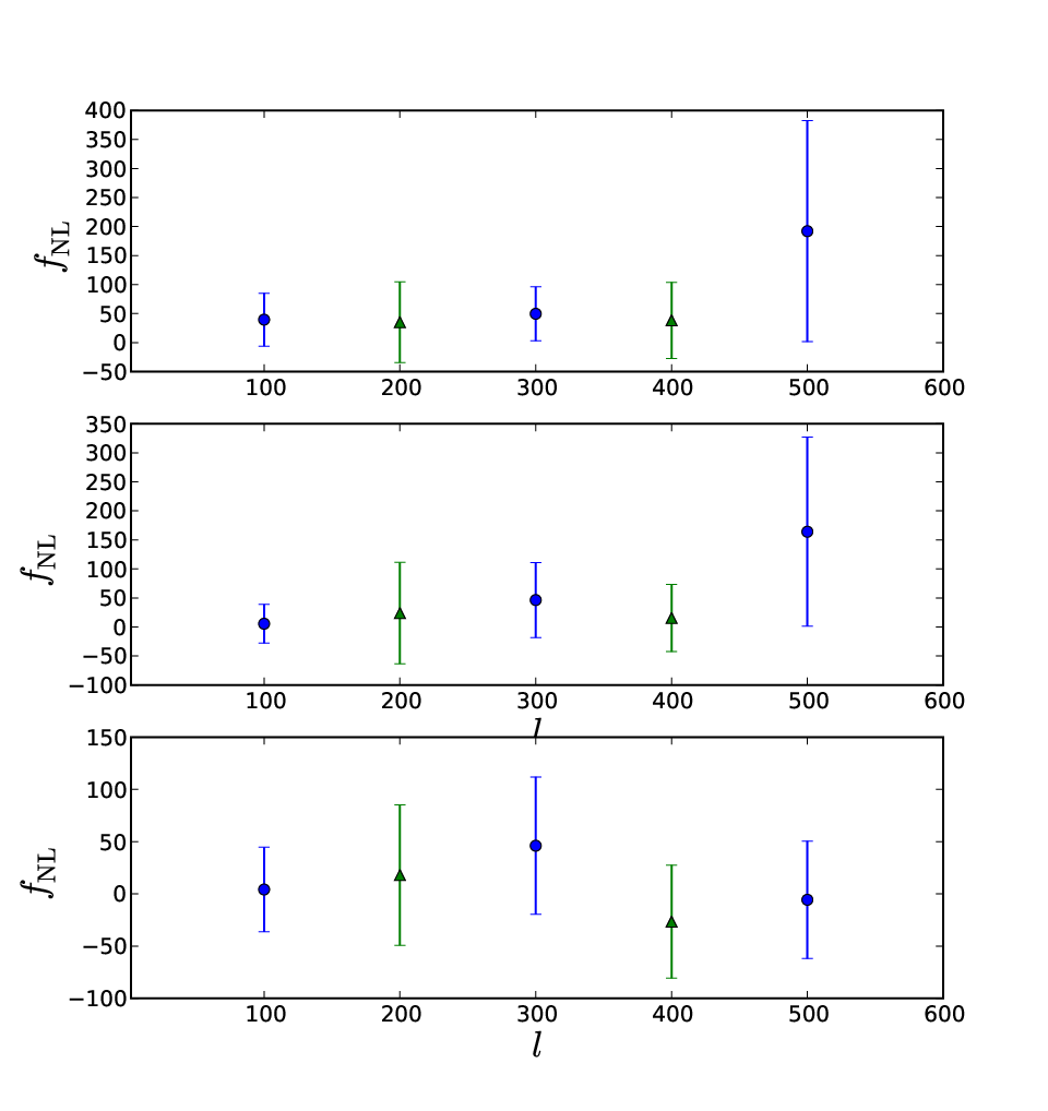
To see if there is any scale dependence to non-Gaussianity we bin in widths of 200 and estimate the value between . The results are shown in Fig. 16 and tabulated in Table IV. Except in the last bin for the case with point sources only between , our values are fully consistent with zero at the 1 level and the last bin is consistent with zero at the 2 level. The last bin also has a large error due to the increase of the instrumental noise. For the same reason, we do not pursue a measurement of when .
It is also interesting to note how accurate our overall error estimate is. As we compute our covariances with 250 simulations there is an inherent error of 1/ in the error bars we obtained in this analysis. Because of this, we note that a more accurate estimate of should be to consider it as where the extra error within the bracket denotes an additional statistical error associated with the finite number of simulations.
| Type | (no PSs) | (w/PSs) | ||||
|---|---|---|---|---|---|---|
| Q | 1.6 | |||||
| V | 0.6 | |||||
| W | 0.6 | |||||
| V+W | 1.0 | |||||
| Q | 1.3 | |||||
| V | 0.3 | |||||
| W | 0.3 | |||||
| V+W | 0.8 | |||||
| Full | ||||||
| Q | 3.2 | |||||
| V | 0.6 | |||||
| W | 0.6 | |||||
| V+W | 0.9 |
| Type | (PS + lensing) | |||||||
|---|---|---|---|---|---|---|---|---|
| Q | 3.4 | |||||||
| V | 1.0 | |||||||
| W | 1.2 | |||||||
| V+W | 1.3 | |||||||
| Q | 0.7 | |||||||
| V | 0.3 | |||||||
| W | 0.3 | |||||||
| V+W | 0.8 | |||||||
| Full | ||||||||
| Q | 3.3 | |||||||
| V | 0.6 | |||||||
| W | 0.8 | |||||||
| V+W | 0.9 |
| Type | (with PSs) | (PSs + lensing-secondary) |
|---|---|---|
| Full | ||
| Technique | Ref | |
|---|---|---|
| WMAP 3-Year, Skewness | [39] | |
| WMAP 5-Year, Skewness | [12] | |
| WMAP 5-Year, Minkowski Functions | [12] | |
| WMAP 5-year, Wavelets | [66] | |
| WMAP 5-year, Needlets | [67] | |
| WMAP 5-year, N-point PDF | [68] | |
| WMAP ISW-correlation | [69] | |
| Large-scale structure bias | [70] | |
| WMAP 5-Year, Optimal Estimator | [40] | |
| WMAP 5-year, Skew-power spectrum | this paper |
V.2 Cross-Skewness
Previous results for from the WMAP 5-year team compute by compressing all information into a single quantity called cross-skewness defined by equation 39. To compare our measurement with their results we calculate our own equivalent version of this cross skewness statistic defined as
| (81) |
where is the estimator obtained from data. We also compute the skewness of the E map using in above. We jointly fit and with a combination of and by effectively comparing the statistic from data to prediction from theory with theory expectation computed as, for example, . In order to determine the errors we also preform the same cross-skewness analysis on all 250 simulations and calculate the covariance of and from these 250 numbers for each frequency. We find that estimated from each of the 250 Gaussian and noise simulations lead to a Gaussian error distribution (Figure 17).
We tabulate our results for after marginalizing over ’s in Table VI. Here, when doing the summations we set so we can compare directly with WMAP 5-year published results [12]. We see that for all three channels we have good agreement with the WMAP team’s 5-year findings. Our best-fit value tends to be bit more positive than quoted by the WMAP team (with in Q, V, and W respectively), but this is a small difference when compared to the large error bar. The errors quoted in the WMAP 5-year paper is consistent with our measurements had we used the skewness statistic. However, as we discussed earlier, fitting to and leads to an improvement in the error estimate of since the shapes of the two skew spectra allow us to break the degeneracies better. Comparing our V+W result using the two spectra to skewness for the same maps, we find that the improvement in the error is roughly 20%.
| Band | WMAP 5-year | |
|---|---|---|
| Q | ||
| V | ||
| W |
VI Conclusion
In this paper, we constrained the primordial non-Gaussianity parameter of the local model using the skewness power spectrum associated with the two-to-one cumulant correlator of cosmic microwave background temperature anisotropies. This bispectrum-related skewness power spectrum was constructed after weighting the temperature maps with the appropriate window functions to form an estimator that probes the multipolar dependence of the underlying bispectrum associated with primordial non-Gaussianity.
We also estimate a separate skewness power spectrum more sensitive to unresolved point sources. When compared to previous attempts at measuring the primordial non-Gaussianity with WMAP data, our estimators have the main advantage that we do not collapse information to a single number. When model fitting two-to-one skewness power spectrum we make use of bispectra generated by primordial non-Gaussianity, radio point sources, and lensing-secondary correlations. W
We analyze Q, V and W-band WMAP 5-year data using the KQ75 mask out to . Using V and W-band data and marginalizing over model parameters related to point sources, our overall and preferred constraint on is 11.0 at the 68% confidence level ( at 95 confidence). Despite previous claims, we find no evidence for a non-zero value of even marginally at the 1 level.
Acknowledgements.
We are grateful to Eiichiro Komatsu, Dipak Munshi, and Kendrick Smith for assistance during various stages of this work. J.S. acknowledges support from a GAANN fellowship. Partial funding of AA and PS was from NSF CAREER AST-0645427.References
- [1] A. H. Guth, Phys. Rev. D 23, 347 (1981).
- [2] A. D. Linde, Phys. Lett. B 108, 389 (1982).
- [3] A. J. Albrecht and P. J. Steinhardt, Phys. Rev. Lett. 48, 1220 (1982).
- [4] K. Sato, Mon. Not. Roy. Astron. Soc. 195, 467 (1981).
- [5] D. Kazanas, Astrophys. J. 241, L59 (1980).
- [6] A. A. Starobinsky, JTEP Lett. 30, 682 (1979).
- [7] A. H. Guth and S. Y. Pi, Phys. Rev. Lett. 49, 1110 (1982).
- [8] J. M. Bardeen, P. J. Steinhardt and M. S. Turner, Phys. Rev. D 28, 679 (1983).
- [9] S. W. Hawking, Phys. Lett. B 115, 295 (1982).
- [10] V. F. Mukhanov, H. A. Feldman and R. H. Brandenberger, Phys. Rept. 215, 203 (1992).
- [11] A. A. Starobinsky, Phys. Lett. B 117, 175 (1982).
- [12] E. Komatsu et al. [WMAP Collaboration], Astrophys. J. Suppl. 180, 330 (2009) [arXiv:0803.0547 [astro-ph]].
- [13] D. Baumann et al. [CMBPol Study Team Collaboration], arXiv:0811.3919 [astro-ph].
- [14] L. F. Abbott and M. B. Wise, Astrophys. J. 282, L47 (1984).
- [15] L. P. Grishchuk, Sov. Phys. JETP 40, 409 (1975) [Zh. Eksp. Teor. Fiz. 67, 825 (1974)].
- [16] [Planck Collaboration], arXiv:astro-ph/0604069.
- [17] J. Bock et al., arXiv:astro-ph/0604101.
- [18] J. Bock et al. [EPIC Collaboration], arXiv:0906.1188 [astro-ph.CO].
- [19] J. Bock et al., arXiv:0805.4207 [astro-ph].
- [20] D. Baumann et al. [CMBPol Study Team Collaboration], arXiv:0811.3911 [astro-ph].
- [21] J. M. Maldacena, JHEP 0305, 013 (2003) [arXiv:astro-ph/0210603].
- [22] M. Sasaki and E. D. Stewart, Prog. Theor. Phys. 95, 71 (1996) [arXiv:astro-ph/9507001].
- [23] D. H. Lyth, K. A. Malik and M. Sasaki, JCAP 0505, 004 (2005) [arXiv:astro-ph/0411220].
- [24] D. H. Lyth and Y. Rodriguez, Phys. Rev. Lett. 95, 121302 (2005) [arXiv:astro-ph/0504045].
- [25] V. Acquaviva, N. Bartolo, S. Matarrese and A. Riotto, Nucl. Phys. B 667, 119 (2003) [arXiv:astro-ph/0209156].
- [26] T. J. Allen, B. Grinstein and M. B. Wise, Phys. Lett. B 197, 66 (1987).
- [27] T. Falk, R. Rangarajan and M. Srednicki, Astrophys. J. 403, L1 (1993) [arXiv:astro-ph/9208001].
- [28] D. S. Salopek and J. R. Bond, Phys. Rev. D 42, 3936 (1990).
- [29] A. Gangui, F. Lucchin, S. Matarrese and S. Mollerach, Astrophys. J. 430, 447 (1994) [arXiv:astro-ph/9312033].
- [30] S. Mollerach, Phys. Rev. D 42, 313 (1990).
- [31] G. Dvali, A. Gruzinov and M. Zaldarriaga, Phys. Rev. D 69, 023505 (2004) [arXiv:astro-ph/0303591].
- [32] A. D. Linde, JETP Lett. 40, 1333 (1984) [Pisma Zh. Eksp. Teor. Fiz. 40, 496 (1984)].
- [33] A. Berera, Phys. Rev. Lett. 75, 3218 (1995) [arXiv:astro-ph/9509049].
- [34] N. Arkani-Hamed, H. C. Cheng, M. A. Luty and S. Mukohyama, JHEP 0405, 074 (2004) [arXiv:hep-th/0312099].
- [35] E. Silverstein and D. Tong, Phys. Rev. D 70, 103505 (2004) [arXiv:hep-th/0310221].
- [36] X. Chen, Phys. Rev. D 72, 123518 (2005) [arXiv:astro-ph/0507053].
- [37] N. Bartolo, E. Komatsu, S. Matarrese and A. Riotto, Phys. Rept. 402, 103 (2004) [arXiv:astro-ph/0406398].
- [38] E. Komatsu and D. N. Spergel, Phys. Rev. D 63, 063002 (2001) [arXiv:astro-ph/0005036].
- [39] A. P. S. Yadav and B. D. Wandelt, Phys. Rev. Lett. 100, 181301 (2008) [arXiv:0712.1148 [astro-ph]].
- [40] K. M. Smith, L. Senatore and M. Zaldarriaga, arXiv:0901.2572 [astro-ph].
- [41] P. Serra and A. Cooray, Phys. Rev. D 77, 107305 (2008) [arXiv:0801.3276 [astro-ph]].
- [42] A. Cooray, Phys. Rev. D 64, 043516 (2001) [arXiv:astro-ph/0105415].
- [43] D. Munshi and A. Heavens, arXiv:0904.4478 [astro-ph.CO].
- [44] D. M. Goldberg and D. N. Spergel, Phys. Rev. D 59, 103002 (1999) [arXiv:astro-ph/9811251].
- [45] A. Cooray and W. Hu, Astrophys. J. 548, 7 (2001) [arXiv:astro-ph/0004151].
- [46] G. Hinshaw, A. J. Banday, C. L. Bennett, K. M. Gorski and A. Kogut, Astrophys. J., 446, 67 (1995)
- [47] P. G. Ferreira, J. Magueijo and K. M. Gorksi, Astrophys. J., 503, 1 (1998); for updates, see also, J. Pando, D. Vallas-Gabaud D. and L. Fang, Phys. Rev. Lett., 79, 1611 (1998); A. J. Banday, S. Zaroubi, S. and K. M. Gorski, Astrophys. J.in press (astro-ph/9908070); B. Bromley and M. Tegmark, Astrophys. J. Lett., 524, L79 (1999)
- [48] A. Cooray, W. Hu and M. Tegmark, Astrophys. J., 540, 1 (2000)
- [49] U. Seljak and M. Zaldarriaga, Astrophys. J., 469, 437 (1996)
- [50] P. Serra, A. Cooray, A. Amblard, L. Pagano and A. Melchiorri, Phys. Rev. D 78, 043004 (2008) [arXiv:0806.1742 [astro-ph]].
- [51] A. Cooray and R. K. Sheth, Phys. Rept. 372, 1 (2002) [arXiv:astro-ph/0206508].
- [52] A. Cooray, Phys. Rev. D 62, 103506 (2000) [arXiv:astro-ph/0005287].
- [53] A. Cooray, Phys. Rev. D 64, 063514 (2001) [arXiv:astro-ph/0105063].
- [54] A. Cooray, Phys. Rev. D 65, 103510 (2002) [arXiv:astro-ph/0112408].
- [55] N. Afshordi, Phys. Rev. D 70, 083536 (2004) [arXiv:astro-ph/0401166].
- [56] E. Komatsu and U. Seljak, Mon. Not. Roy. Astron. Soc. 336, 1256 (2002) [arXiv:astro-ph/0205468].
- [57] A. Mangilli and L. Verde, arXiv:0906.2317 [astro-ph.CO].
- [58] D. Hanson, K. M. Smith, A. Challinor and M. Liguori, arXiv:0905.4732 [astro-ph.CO].
- [59] A. Cooray, D. Sarkar and P. Serra, Phys. Rev. D 77, 123006 (2008) [arXiv:0803.4194 [astro-ph]].
- [60] M. Veneziani et al., arXiv:0904.4313 [astro-ph.CO].
- [61] G. Chen and I. Szapudi, Astrophys. J. 647, L87 (2006) [arXiv:astro-ph/0606394].
- [62] E. Komatsu, D. N. Spergel and B. D. Wandelt, Astrophys. J. 634, 14 (2005) [arXiv:astro-ph/0305189].
- [63] K. M. Gorski, E. Hivon, A. J. Banday, B. D. Wandelt, F. K. Hansen, M. Reinecke and M. Bartelman, Astrophys. J. 622, 759 (2005) [arXiv:astro-ph/0409513].
- [64] N. Jarosik et al. [WMAP Collaboration], Astrophys. J. Suppl. 170, 263 (2007) [arXiv:astro-ph/0603452].
- [65] G. Hinshaw et al. [WMAP Collaboration], Astrophys. J. Suppl. 180, 225 (2009) [arXiv:0803.0732 [astro-ph]].
- [66] A. Curto, E. Martinez-Gonzalez and R. B. Barreiro, arXiv:0902.1523 [astro-ph.CO].
- [67] O. Rudjord, F. K. Hansen, X. Lan, M. Liguori, D. Marinucci and S. Matarrese, arXiv:0901.3154 [astro-ph.CO].
- [68] P. Vielva and J. L. Sanz, arXiv:0812.1756 [astro-ph].
- [69] N. Afshordi and A. J. Tolley, Phys. Rev. D 78, 123507 (2008) [arXiv:0806.1046 [astro-ph]].
- [70] A. Slosar, C. Hirata, U. Seljak, S. Ho and N. Padmanabhan, JCAP 0808, 031 (2008) [arXiv:0805.3580 [astro-ph]].