跳到论文正文
W Papers独立论文阅读器 arXiv:0907.3947 论文正文 计算阅读时间 · 0%
引用这篇论文根据当前论文元数据生成,正式投稿前建议核对。


License: arXiv.org perpetual non-exclusive license
arXiv:0907.3947v2 [hep-ph] 28 Jul 2009

SUSY radiative corrections on μ−τ\mu-\tau neutrino refraction including possible R-parity breaking interactions

J. Gava Email: gava@ipno.in2p3.fr Affiliation: Institut de Physique Nucléaire, CNRS/IN2P3 UMR 8608 and Université Paris-Sud 11, Bât. 100,
F-91406 Orsay cedex, France
   C.-C. Jean-Louis Email: charles.jean-louis@th.u-psud.fr Affiliation: Laboratoire de Physique Théorique, CNRS UMR 8627, Bât. 210, Université Paris-Sud 11, 91405 Orsay Cedex, France
22th July 2009
Abstract

In this paper we investigate the one-loop radiative corrections to the neutrino indices of refraction from supersymmetric models. We consider the Next-to Minimal Supersymmetric extension of the Standard Model (NMSSM) which happens to be a better supersymmetric candidate than the MSSM for both theoretical and experimental reasons. We scan the relevant SUSY parameters and identify regions in the parameter space which yield interesting values for Vμ​τV_{\mu\tau}. If R-parity is broken there are significant differences between MSSM and NMSSM contributions contrary to the R-parity conserved case. Finally, for a non-zero CP-violating phase, we show analytically that the presence of Vμ​τV_{\mu\tau} will explicitly imply CP-violation effects on the supernova electron (anti-) neutrino fluxes.

Keywords: 
Core-collapse Supernova, Neutrino Physics, Supersymmetry, R-parity violation
pacs
14.60.Pq, 11.30.Pb, 97.60.Bw, 11.30.Er, 11.30.Fs

I Introduction

The charged current interaction between neutrinos and their associated leptons in medium give an effective matter potential which can lead to a resonant flavour conversion called the Mikheyev-Smirnov-Wolfenstein (MSW) effect [1, 2]. Such behaviour solves elegantly the solar neutrino deficit problem first pointed out by pioneering experiment of R. Davis in the 60’s [3]. Such phenomenon is of crucial importance for the propagation of neutrinos in the supernova environment whose flux detection could yield precious information concerning the dynamics of the density profile or fundamental neutrinos properties like the hierarchy or the value of the third mixing angle. In supernovae, depending on the mass hierarchy, the electron neutrino may encounter one or two resonances via charged current, while the muon or tau neutrinos will only interact via neutral current, indistinguishably at the tree level in the Standard Model (SM). Indeed, due to the absence of muon or tau particle in such environment, coherent forward scattering may only intervene via neutral current to which all flavours are sensitive. Considering that matter interaction can also be seen as neutrino index of refraction [4, 5], Botella et al. [6], after showing that correction at O⁡(α)O\left(\alpha\right) were negligible in the case of a neutral medium [7], proved that differences at one-loop in the neutrino index of refraction could arise for muon and tau neutrinos at order O⁡(απ​sin2⁡θW​mτ2MW2)O\left({\alpha\over\pi\sin^{2}\theta_{W}}{m_{\tau}^{2}\over M_{W}^{2}}\right). Later, supersymmetric radiative corrections, in the case of the minimal supersymmetric model (MSSM) has been partially calculated [8] showing that it could give potentially much larger radiative effects than in the SM. It is interesting to note that such radiative corrections have been for a longtime considered as negligible or without observable consequences for the supernova environment. Such consideration was probably true when not taking into account the neutrino-neutrino interaction which has dramatically changed the vision we have of neutrino propagating in an exploding star and which has gone through an intense investigation [9, 10, 11, 12, 13, 14, 15, 16, 17, 18, 19, 20, 21, 22, 23, 24, 25, 29, 30, 26, 27, 28, 31, 32, 33]. Actually few papers have shown the importance of the one-loop correction in addition with the neutrino-neutrino interaction. First it has been shown that for early time after post-bounce when the matter density profile is very high, neutrinos can encounter the μ−τ\mu-\tau resonance and possibly modify the νe\nu_{e} flux [25, 27]. Unfortunately, it has also been shown that in such case the high density in addition with a multi-angle neutrino-neutrino interaction would make those effects vanish [31]. Besides those works, only one paper11 1 In [27], it was noted that the CP-violating phase could influence sensibly the μ\mu and τ\tau neutrino flavor. [29] has shown the importance of Vμ​τV_{\mu\tau} via the influence of the CP-violating phase δ\delta contained in the MNSP matrix and whose value is still unknown. Such term induces effects of a non-zero CP-violating phase on the electron neutrino fluxes inside and outside the supernova.

The goal of this paper is to calculate such corrections in the SUSY framework with and without taking into account R-parity breaking interactions. It is organized as follows: Sec.2 introduces the theoretical framework where we briefly remember how to calculate radiative corrections in this context and more importantly where we introduce the supersymmetric framework. The corrections with R-parity conservation are calculated in Sec.3 and Sec.4 is dedicated to the case where the R-parity is broken. Before concluding, we explicitly demonstrate in Sec.5 the influence of Vμ​τV_{\mu\tau} on the νe\nu_{e} flux when the CP-violating phase is non-zero.

II Theoretical framework

II.1 The calculations of the radiative corrections

Neutrinos interaction through matter can be described using indices of refraction and in this case, the evolution equation of neutrinos with matter, omitting the neutrino-neutrino interaction is:

i​dd​t​(νeνμντ)=[12​pν​U​(Δ​m1220000000Δ​m322)​U†−pν​(Δ​ne​μ0000000Δ​nτ​μ)]​(νeνμντ),i{d\over dt}\left(\begin{array}[]{r}\nu_{e}\\ \nu_{\mu}\\ \nu_{\tau}\end{array}\right)=\left[{1\over 2p_{\nu}}U\left(\begin{array}[]{ccc}\Delta m^{2}_{12}&0&0\\ 0&0&0\\ 0&0&\Delta m^{2}_{32}\end{array}\right)U^{\dagger}-p_{\nu}\left(\begin{array}[]{ccc}\Delta n_{e\mu}&0&0\\ 0&0&0\\ 0&0&\Delta n_{\tau\mu}\end{array}\right)\right]\left(\begin{array}[]{r}\nu_{e}\\ \nu_{\mu}\\ \nu_{\tau}\end{array}\right), (1)

where UU is the MNSP matrix, pνp_{\nu} the neutrino momentum, Δ​mi​j2≡mνi2−mνj2\Delta m^{2}_{ij}\equiv m_{\nu_{i}}^{2}-m_{\nu_{j}}^{2} and Δ​nα​β≡nνα−nνβ\Delta n_{\alpha\beta}\equiv n_{\nu_{\alpha}}-n_{\nu_{\beta}}.

To size the effect of such radiative correction on the neutrino propagation, we study the one-loop effect on the scattering amplitude matrix which describes the interaction of neutrinos with matter:

M⁡(νℓ​f→νℓ​f)=−i​GF2​ν¯ℓ​γρ​(1−γ5)​νℓ​f¯​γρ​(Cνℓ​fV+Cνℓ​fA​γ5)​f.M(\nu_{\ell}f\to\nu_{\ell}f)=-i{G_{F}\over\sqrt{2}}\bar{\nu}_{\ell}\gamma^{\rho}(1-\gamma_{5})\nu_{\ell}\bar{f}\gamma_{\rho}(C^{V}_{\nu_{\ell}f}+C^{A}_{\nu_{\ell}f}\gamma_{5})f. (2)

In the calculations we will use the same approximations as in [6] and [8] i.e, neutrinos are propagating though an unpolarized medium at rest. Consequently, the neutrino index of refraction can be written as:

pν(nνℓ−1)=−2GF∑f=u,d,eCνℓ​fVNf.p_{\nu}(n_{\nu_{\ell}}-1)=-\sqrt{2}G_{F}\sum_{f=u,d,e}C^{V}_{\nu_{\ell}f}N_{f}. (3)

where NfN_{f} is the number density of fermion ff in the medium. Therefore, the interesting parameter to study in order to size the radiative correction to matter interaction is Cνℓ​fVC^{V}_{\nu_{\ell}f} which is defined at the tree-level by

Cνℓ​fV=T3​(fL)−2​Qf​sin2⁡θW+δℓ​f,C^{V}_{\nu_{\ell}f}=T_{3}(f_{L})-2Q_{f}\sin^{2}\theta_{W}+\delta_{\ell f}, (4)

with sin2⁡θW≡1−mW2/mZ2≃0.23\sin^{2}\theta_{W}\equiv 1-m_{W}^{2}/m_{Z}^{2}\simeq 0.23, while QfQ_{f} and T3​(fL)T_{3}(f_{L}) are respectively the electric charge and the third component of the weak isospin of the fermion fLf_{L}. To parametrize the loop corrections to Cνℓ​fVC^{V}_{\nu_{\ell}f} Botella et al. [6] have defined in some kind of an arbitrary but convenient way a new Cνℓ​fVC^{V}_{\nu_{\ell}f} by

Cνℓ​fV=ρνℓ​f​T3​(fL)−2​Qf​λνℓ​f​sW2.C^{V}_{\nu_{\ell}f}=\rho^{\nu_{\ell}f}T_{3}(f_{L})-2Q_{f}\lambda^{\nu_{\ell}f}s_{W}^{2}. (5)

for f≠ℓf\neq\ell where the ρνℓ​f\rho^{\nu_{\ell}f} includes the f-dependent (box) diagrams contributions. Since the λνℓ​f\lambda^{\nu_{\ell}f} are chosen to be independent of the ff, in a electrically neutral medium, they will not contribute to Δ​nτ​μ\Delta n_{\tau\mu}. Consequently, Δ​nτ​μ\Delta n_{\tau\mu} will only be sensitive to Δ​ρf≡ρντ​f−ρνμ​f\Delta\rho^{f}\equiv\rho^{\nu_{\tau}f}-\rho^{\nu_{\mu}f}. Note that we are only interested about the difference between nνμn_{\nu_{\mu}} and nντn_{\nu_{\tau}} indices of refraction because the loop correction to Δne​μ=−2GFNe/pν\Delta n_{e\mu}=-\sqrt{2}G_{F}N_{e}/p_{\nu} will be negligible since electron neutrinos already encounter charged current interactions with matter. In the SM, the correction have been calculated and are found to be small :

Δ​nτ​μ=Vμ​τ=ε​Ve≃5.4×10⁻⁵​Ve\Delta n_{\tau\mu}=V_{\mu\tau}=\varepsilon V_{e}\simeq 5.4\times 10^{-5}\,V_{e} (6)

where Vμ​τV_{\mu\tau} is the effective matter potential to tau neutrinos due to one-loop corrections and ε\varepsilon the ratio between the Vμ​τV_{\mu\tau} and VeV_{e} which yields the size of the loop correction in comparison with the charged-current matter potential for electron neutrinos VeV_{e}.

II.2 The supersymmetric framework

The most significant theoretical issues of the Standard Model (SM) are the hierarchy problem for the Higgs mass and the non-unification of the gauge couplings . Supersymmetry allows us to address these problems and is an attractive candidate for new physics beyond the Standard Model (SM). In this theory a supersymmetric particle called LSP (Lightest Supersymmetric Particle) is a natural candidate for dark matter. Among various supersymmetric models the most extensively studied is the minimal supersymmetric model (MSSM).

The MSSM contains the minimum number of fields to describe the known SM particles and their superpartners. These fields can be gathered into chiral superfiels and vector superfields. A chiral superfield Φ^\hat{\Phi} is a multiplet which contains a scalar field (zz), a fermionic field (ψ\psi) and an auxiliary field (FF): Φ^\hat{\Phi} = (zz, ψ\psi, FF). A vector superfield V^\hat{V} is a multiplet which contains a bosonic field (vμv^{\mu}), a fermionic field (λ\lambda) and an auxiliary field (DD): V^\hat{V} = (vμv^{\mu}, λ\lambda, DD). FF and DD are auxiliary fields, they do not have kinetic terms. They are eliminated by the minimization equations of the Lagragian. To SM fermionic fields (leptons, quarks), we have supersymmetric scalar fields (sleptons, squarks) associated. Concerning SM vector bosons (U​(1)YU(1)_{Y}, S​U​(2)LSU(2)_{L}, S​U​(3)CSU(3)_{C} gauge bosons), fermionic fields called gauginos (bino, winos, gluinos) are associated to. Finally, we have fermionic fields called higgsinos associated to Higgs bosons. Higgsinos and gauginos will mix to generate neutralinos and charginos.

A superfield is a function of spacetime coordinates and so-called superspace coordinates which appear as anticommuting Grassman variables [34]. It can be expanded in terms of its component fields and these Grassman variables. Products of superfields can be developed resulting in products of individual particle and sparticle fields.

We call superpotential all the renormalizable products of chiral superfields in a given supersymmetric model. The MSSM’s superpotential is:

WM​S​S​M=ht​Q^.H^u​T^Rc−hb​Q^.H^d​B^Rc−hτ​L^.H^d​L^Rc+μ​H^u.H^d\begin{array}[]{rcl}{\it{W}}_{MSSM}&=&h_{t}\hat{Q}.\hat{H}_{u}\hat{T}_{R}^{c}-h_{b}\hat{Q}.\hat{H}_{d}\hat{B}_{R}^{c}-h_{\tau}\hat{L}.\hat{H}_{d}\hat{L}_{R}^{c}\\ &+&\mu\hat{H}_{u}.\hat{H}_{d}\end{array} (7)

where H^u,Q^​…\hat{H}_{u},\hat{Q}... are chiral superfields. The fermionic part of the supersymmetric lagrangian is obtained through a procedure where the superfields of the superpotential are expanded in terms of component fields and then the superspace coordinates of the result are integrated out:

ℒM​S​S​M=ht​ψQ.Hu​ψTRc−hb​ψQ.Hd​ψBRc−hτ​ψL.Hd​ψLRc+μψHu.ψHd+…(+h.c)\begin{array}[]{rcl}{\cal{L}}_{MSSM}&=&h_{t}\psi_{Q}.H_{u}\psi_{T_{R}^{c}}-h_{b}\psi_{Q}.H_{d}\psi_{B_{R}^{c}}-h_{\tau}\psi_{L}.H_{d}\psi_{L_{R}^{c}}\\ &&+\mu\psi_{H_{u}}.\psi_{H_{d}}+\ldots(+h.c)\end{array} (8)

In Supersymmetry, we need two Higgs bosons to give masses to the other particles.

Despite its simplicity, there are two unexplained hierarchies, within the MSSM:

  • -

    the so-called μ\mu-problem [35]. It arises from the presence of a mass μ\mu-term for the Higgs fields in the superpotential. The only two theoretical natural values for this parameter are either zero or the Planck energy scale. However, we need μ≳100​G​e​V\mu\gtrsim 100GeV to satisfy LEP constraints on the chargino masses and μ≲MS​U​S​Y\mu\lesssim M_{SUSY} for a destabilization of the Higgs potential in order to have non-vanishing v.e.v. for the scalar Higgs fields (<Hu,d>≠0<H_{u,d}>\neq 0)

  • -

    The other hierarchy with an unknown origin is the one existing between the small neutrino masses (smaller than the eV scale) and the electroweak symmetry breaking scale (∼100​G​e​V\sim 100GeV).

In this paper, our framework is the Next-to Minimal Supersymmetric extension of the Standard Model (NMSSM) [36]. This model provides an elegant solution to the μ\mu-problem via the introduction of a new gauge-singlet superfield S^\hat{S} that acquires naturally a v.e.v. xx of the order of the supersymmetry breaking scale, generating an effective μ\mu parameter (λ​x=μeff\lambda x=\mu_{\rm eff}) of order of the electroweak scale. Furthermore, this model explains the second hierarchy by generating two neutrino masses at tree level through R-parity breaking [37] as we will see below.

The NMSSM’s superpotential is:

WN​M​S​S​M=ht​Q^.H^u​T^Rc−hb​Q^.H^d​B^Rc−hτ​L^.H^d​L^Rc+λ​S^​H^u.H^d+κ3​S^3.\begin{array}[]{rcl}{\it{W}}_{NMSSM}&=&h_{t}\hat{Q}.\hat{H}_{u}\hat{T}_{R}^{c}-h_{b}\hat{Q}.\hat{H}_{d}\hat{B}_{R}^{c}-h_{\tau}\hat{L}.\hat{H}_{d}\hat{L}_{R}^{c}\\ &+&\lambda\hat{S}\hat{H}_{u}.\hat{H}_{d}+\frac{\kappa}{3}\hat{S}^{3}.\end{array} (9)

Then, the fermionic part of the NMSSM lagrangian is:

ℒN​M​S​S​M=ht​ψQ.Hu​ψTRc−hb​ψQ.Hd​ψBRc−hτ​ψL.Hd​ψLRc+λSψHu.ψHd+κSψSψS+…(+h.c)\begin{array}[]{rcl}{\cal{L}}_{NMSSM}&=&h_{t}\psi_{Q}.H_{u}\psi_{T_{R}^{c}}-h_{b}\psi_{Q}.H_{d}\psi_{B_{R}^{c}}-h_{\tau}\psi_{L}.H_{d}\psi_{L_{R}^{c}}\\ &&+\lambda S\psi_{H_{u}}.\psi_{H_{d}}+\kappa S\psi_{S}\psi_{S}+\ldots(+h.c)\end{array} (10)

The NMSSM contains the following particles:

  • .

    Standard Model fermions and their left and right scalar supersymmetric partners (sfermions)

  • .

    Standard Model gauge bosons

  • .

    3 neutral scalar Higgs (h1h_{1}, h2h_{2}, h3h_{3})

  • .

    2 neutral pseudo-scalar Higgs (a1a_{1}, a2a_{2})

  • .

    1charged Higgs (H±H^{\pm})

  • .

    2 charginos (χ1,2±\chi_{1,2}^{\pm}) originally from mixing between charged fermionic superpartners of the gauge bosons (gauginos) and charged fermionic superpartners of Higgs bosons (higgsinos)

  • .

    5 neutralinos (χ1​…​50\chi^{0}_{1\ldots 5}) of which the lighest called lighest supersymmetric particle (LSP) is gererally stable and is thence a natural candidate for Dark Matter. They come from the mixing between neutral gauginos et neutral higgsinos.

The NMSSM phenomenology contains the MSSM phenomenology if we take λ→0\lambda\rightarrow 0, κ→0\kappa\rightarrow 0 by keeping μeff\mu_{\rm eff} of the order of MWM_{W}.

Experimental limits on supersymmetric particle masses obviously show that SUSY has to be broken. Thus, the supersymmetric particle masses will be different from Standard Model particle masses. The soft SUSY breaking terms in the NMSSM are:

  • a)

    mass terms for scalar particles:

    mHu2​|Hu|2+mHd2​|Hd|2+mS2​|S|2+mQ32​|Q3|2+mt~R2​|TR|2+mb~R2​|BR|2+mL32​|L3|2+mτ~R2​|LR|2+…m^{2}_{H_{u}}|H_{u}|^{2}+m^{2}_{H_{d}}|H_{d}|^{2}+m^{2}_{S}|S|^{2}+m^{2}_{Q_{3}}|Q_{3}|^{2}+m^{2}_{\tilde{t}_{R}}|T_{R}|^{2}+m^{2}_{\tilde{b}_{R}}|B_{R}|^{2}+m^{2}_{L_{3}}|L_{3}|^{2}+m^{2}_{\tilde{\tau}_{R}}|L_{R}|^{2}+\ldots

    where all the fields are scalar fields,

  • b)

    mass terms for gauginos:

    12​M1​λ1​λ1+12​M2​λ2→.λ2→+12​M3​λ3→.λ3→\frac{1}{2}M_{1}\lambda_{1}\lambda_{1}+\frac{1}{2}M_{2}\overrightarrow{\lambda_{2}}.\overrightarrow{\lambda_{2}}+\frac{1}{2}M_{3}\overrightarrow{\lambda_{3}}.\overrightarrow{\lambda_{3}}
  • c)

    soft terms associated to the superpotential:

    λAλSHu.Hd+κ3AκS3+htAtQ.HuTRc−hbAbQ.HdBRc−hτAτL.HdLRc+…(+h.c)\lambda A_{\lambda}SH_{u}.H_{d}+\frac{\kappa}{3}A_{\kappa}S^{3}+h_{t}A_{t}Q.H_{u}T_{R}^{c}-h_{b}A_{b}Q.H_{d}B_{R}^{c}-h_{\tau}A_{\tau}L.H_{d}L_{R}^{c}+\ldots(+h.c)

    where all fields are scalar fields.

III R-parity conserved SUSY corrections

In Supersymmetry, one usually considers all sfermions to be exactly degenerate at the GUT scale, and obtain their low energy splittings from the renormalization group evolution of the soft parameters and from terms arising after the electroweak symmetry breaking. In this way, although squarks become significantly split from sleptons, the splittings among the masses of different slepton generations are only due to the small τ\tau-Yukawa coupling. This usually implies that mτ~2−mμ~2m_{\tilde{\tau}}^{2}-m_{\tilde{\mu}}^{2} is O⁡(mτ2)O(m_{\tau}^{2}), and hence the radiative effects on the νμ,τ\nu_{\mu,\tau} indices of refraction are, in this case, not larger than the SM ones. In the following, we shall consider in the following a large τ~L\tilde{\tau}_{L}–τ~R\tilde{\tau}_{R} mixing. This occurs for large values of the effective μ\mu parameter and tanβ\beta, or for large values of the parameter AA of the trilinear soft terms, in which case the splitting can be O[mτ(Aτ+μefftanβO[m_{\tau}(A_{\tau}+\mu_{\rm eff}tan\beta)] as we can see below.

We give here the stau and smuon mass-squared matrices where we neglect splittings due to DD-terms among charged and neutral sleptons or among ℓ~L\tilde{\ell}_{L} and ℓ~R\tilde{\ell}_{R}. The diagonal terms are respectively the ℓ~R\tilde{\ell}_{R} and ℓ~L\tilde{\ell}_{L} mass-squared terms.

For tau sleptons:

ℳτ~2=(mτ2+mτ~R2mτ​(Aτ+μeff​t​a​n​β)mτ​(Aτ+μeff​t​a​n​β)mτ2+mL32),\displaystyle{\cal{M}}^{2}_{\tilde{\tau}}=\left(\begin{array}[]{cc}m_{\tau}^{2}+m_{\tilde{\tau}_{R}}^{2}&m_{\tau}(A_{\tau}+\mu_{\rm eff}tan\beta)\cr m_{\tau}(A_{\tau}+\mu_{\rm eff}tan\beta)&m_{\tau}^{2}+m_{L_{3}}^{2}\end{array}\right)\ ,\

and for muon sleptons:

ℳμ~2=(mμ2+mμ~R2mμ​(Aμ+μeff​t​a​n​β)mμ​(Aμ+μeff​t​a​n​β)mμ2+mL22)\displaystyle{\cal{M}}^{2}_{\tilde{\mu}}=\left(\begin{array}[]{cc}m_{\mu}^{2}+m_{\tilde{\mu}_{R}}^{2}&m_{\mu}(A_{\mu}+\mu_{\rm eff}tan\beta)\cr m_{\mu}(A_{\mu}+\mu_{\rm eff}tan\beta)&m_{\mu}^{2}+m_{L_{2}}^{2}\end{array}\right)

where

  • -

    mτ~R2m_{\tilde{\tau}_{R}}^{2}, mμ~R2m_{\tilde{\mu}_{R}}^{2}, mL32m_{L_{3}}^{2} and mL22m_{L_{2}}^{2} are of the order of Ms​u​s​y2∼0.1−1​T​e​V2M_{susy}^{2}\sim 0.1-1TeV^{2},

  • -

    (Aτ+μeff​t​a​n​βA_{\tau}+\mu_{\rm eff}tan\beta), (Aμ+μeff​t​a​n​βA_{\mu}+\mu_{\rm eff}tan\beta) are of the order of Ms​u​s​yM_{susy},

  • -

    mτ=1.8​G​e​Vm_{\tau}=1.8GeV, mμ=105​M​e​Vm_{\mu}=105MeV.

In the 2n​d2^{nd} generation case, we can neglect the mixing between μ~R\tilde{\mu}_{R} and μ~L\tilde{\mu}_{L} because the off-diagonal terms are negligible w.r.t. the diagonal terms. But in the third generation, we have to consider τ~1\tilde{\tau}_{1}, τ~2\tilde{\tau}_{2} instead of τ~R\tilde{\tau}_{R}, τ~L\tilde{\tau}_{L}.

The SUSY contribution to Δ​nτ​μ\Delta n_{\tau\mu} can then be larger than the SM one.

In the following, to calculate the loop diagrams contributions we will use the dimensional regularization method and the vanishing external legs approximation [6, 8] which turns out to be legitimate because of the low masses and energy of the fermions with respect to the electro-weak (MWM_{W}) and SUSY (MS​U​S​YM_{SUSY}) breaking scales. When one does not use this approximation, the loop integrals to perform will have several different mass scales. Such calculations are much more complicated and need advanced mathematical methods as in [38]. In this framework, some specific functions will appear:

  • -

    For the self-energies and the penguin:

    H0​(x,y)=x​y​[x​ln​x(x−y)​(x−1)+(x↔y)],H_{0}(x,y)=\sqrt{xy}\left[{x{\rm ln}x\over(x-y)(x-1)}+(x\leftrightarrow y)\right],
    G0​(x,y)=[x2​ln​x(x−y)​(x−1)+(x↔y)].G_{0}(x,y)=\left[{x^{2}{\rm ln}x\over(x-y)(x-1)}+(x\leftrightarrow y)\right].
  • -

    For the box diagrams:

    H′​(x,y,z)=x​y​[x​ln​x(x−y)​(x−z)​(x−1)+y​ln​y(y−x)​(y−z)​(y−1)+z​ln​z(z−x)​(z−y)​(z−1)],H^{\prime}(x,y,z)=\sqrt{xy}\left[{x{\rm ln}x\over(x-y)(x-z)(x-1)}+{y{\rm ln}y\over(y-x)(y-z)(y-1)}+{z{\rm ln}z\over(z-x)(z-y)(z-1)}\right],
    G′​(x,y,z)=x2​ln​x(x−y)​(x−z)​(x−1)+y2​ln​y(y−x)​(y−z)​(y−1)+z2​ln​z(z−x)​(z−y)​(z−1).G^{\prime}(x,y,z)={x^{2}{\rm ln}x\over(x-y)(x-z)(x-1)}+{y^{2}{\rm ln}y\over(y-x)(y-z)(y-1)}+{z^{2}{\rm ln}z\over(z-x)(z-y)(z-1)}.

III.1 Vertices

Following the notation of [39, 40], we denote by Ni​jN_{ij} by χi0≡Ni​j​Ψ~j\chi_{i}^{0}\equiv N_{ij}\tilde{\Psi}_{j} where Ψ~T=(B~,W~3,h~u,h~d,s~)\tilde{\Psi}^{T}=(\tilde{B},\tilde{W}_{3},\tilde{h}_{u},\tilde{h}_{d},\tilde{s}), UU and VV are the 2×22\times 2 matrices required for the diagonalization of the chargino mass matrix.

Refer to caption

Figure 1: R-parity conserved vertices involving charginos and up fermions.

Refer to caption

Figure 2: R-parity conserved vertices involving charginos and down fermions.

We see in Fig.(1) and (2) that vertices between chargino χi+\chi_{i}^{+}, a fermion ff and the right scalar partner f~R\tilde{f}_{R} are negligible w.r.t. vertices between chargino χi+\chi_{i}^{+}, a fermion ff and the left scalar partner f~L\tilde{f}_{L} because mfMW≪1\frac{m_{f}}{M_{W}}\ll 1 for f≡μ,u,df\equiv\mu,u,d. We will neglect the loops including the primary vertices below.

Refer to caption

Figure 3: R-parity conserved vertices involving neutralinos, fermions and associated sfermions.

Refer to caption

Figure 4: R-parity conserved vertices with Z0Z^{0}-boson.

The coupling of one neutralino χi0\chi_{i}^{0} to one fermion and the associated left (right) scalar partner Gf​L​(R)jG^{j}_{fL(R)} is:

Gf​Lj=Qf​s​i​n​θW​Nj​1∗+cLfc​o​s​θW​Nj​2∗G^{j}_{fL}=Q_{f}sin\theta_{W}N^{*}_{j1}+{c_{L}^{f}\over cos\theta_{W}}N^{*}_{j2}

where f≡ν,e,u,df\equiv\nu,e,u,d.

Gf​Rj=sign⁡(mχj0)​[Qf​s​i​n​θW​Nj​1+cRfc​o​s​θW​Nj​2]G^{j}_{fR}={\rm sign}(m_{\chi^{0}_{j}})\left[Q_{f}sin\theta_{W}N_{j1}+{c_{R}^{f}\over cos\theta_{W}}N_{j2}\right]

where f≡e,u,df\equiv e,u,d.

The coupling of left (right) scalar partners to the Z0Z^{0}-boson is:

cL⁡(R)f=T3​(fL⁡(R))−Qf​s​i​n2​θW.c^{f}_{L(R)}=T_{3}(f_{L(R)})-Q_{f}sin^{2}\theta_{W}.

The coupling of scalar partners in their mass basis to the Z0Z^{0}-boson [41] is:

cf​Mk​j=T3(f)∑i=13Γf​Lk​iΓf​Lji∗−Qfsin2θWδk​hc^{kj}_{f\it{M}}=T_{3}(f)\sum_{i=1}^{3}\Gamma_{fL}^{ki}\Gamma_{fL}^{ji*}-Q_{f}sin^{2}\theta_{W}\delta^{kh}

where τ~L=Γτ​Lk​3​τ~k\tilde{\tau}_{L}=\Gamma_{\tau L}^{k3}\tilde{\tau}_{k}. The coupling of charginos to the Z0Z^{0}-boson [41, 42], is:

𝒪′i​jL=−Vi​1​Vj​1∗−12​Vi​2​Vj​2∗+δi​j​s​i​n2​θW{\cal O^{\prime}}^{L}_{ij}=-V_{i1}V^{*}_{j1}-\frac{1}{2}V_{i2}V^{*}_{j2}+\delta_{ij}sin^{2}\theta_{W}

and

𝒪′i​jR=−Ui​1​Uj​1∗−12​Ui​2​Uj​2∗+δi​j​s​i​n2​θW.{\cal O^{\prime}}^{R}_{ij}=-U_{i1}U^{*}_{j1}-\frac{1}{2}U_{i2}U^{*}_{j2}+\delta_{ij}sin^{2}\theta_{W}.

We will assume below that all the parameters are real.

III.2 Self-energy diagrams

The computation of the supersymmetric contribution to Δ​ρ\Delta\rho requires the evaluation of the Feynman diagrams.

The self-energy, penguin and box contributions to Δ​ρf\Delta\rho^{f} can be written as

Δ​ρf=Δ​ρp+Δ​ρb​o​xfT3​(fL).\Delta\rho^{f}=\Delta\rho_{p}+{\Delta\rho^{f}_{box}\over T_{3}(f_{L})}.

We consider here the contributions to neutrino and antineutrino scattering involving self-energy diagrams.

The first contribution implies a slepton-chargino loop (Fig.5α\alpha). We diagonalize the stau mass matrix and use the vertices of Fig.(1). We neglect the μ~R\tilde{\mu}_{R} contribution.

Δρℓ~(Σ)=−αW8​π∑j=12Uj​12[∑k=12Γτ​Lk​32{G0(Xχj+​τ~k,1)+lnmτ~k2μ2}−{G0(Xχj+​μ~L,1)+lnmμ~L2μ2}]\begin{array}[]{rcl}\Delta\rho^{\tilde{\ell}}(\Sigma)=-{\alpha_{W}\over 8\pi}\sum_{j=1}^{2}U_{j1}^{2}&&\left[\sum_{k=1}^{2}{\Gamma_{\tau L}^{k3}}^{2}\left\{G_{0}(X_{\chi^{+}_{j}\tilde{\tau}_{k}},1)+{\rm ln}{m_{\tilde{\tau}_{k}}^{2}\over\mu^{2}}\right\}\right.\\ &&\left.-\left\{G_{0}(X_{\chi^{+}_{j}\tilde{\mu}_{L}},1)+{\rm ln}{m_{\tilde{\mu}_{L}}^{2}\over\mu^{2}}\right\}\right]\end{array} (17)

where Xa​b=ma2mb2X_{ab}=\frac{m_{a}^{2}}{m_{b}^{2}}. Then, we have a neutralino-sneutrino loop (Fig.6ι\iota).

Δρν~(Σ)=−αW4​π∑j=15Gν​Lj2{G0(Xχj0​ν~τL,1)+lnmν~τL2μ2−(ν~τL→ν~μL)}.\displaystyle\Delta\rho^{\tilde{\nu}}(\Sigma)=-{\alpha_{W}\over 4\pi}\sum_{j=1}^{5}{G_{\nu L}^{j}}^{2}\left\{G_{0}(X_{\chi^{0}_{j}\tilde{\nu}_{\tau_{L}}},1)+{\rm ln}{m_{\tilde{\nu}_{\tau_{L}}}^{2}\over\mu^{2}}-(\tilde{\nu}_{\tau_{L}}\to\tilde{\nu}_{\mu_{L}})\right\}. (18)

Refer to caption

Figure 5: R-parity conserved penguins and self-energies involving charginos and the charged Higgs.

III.3 penguin diagrams

We consider here the contributions to (anti)neutrino scattering involving penguins. We use the vertices of Fig.(4).

Refer to caption

Figure 6: R-parity conserved penguins and self-energies involving neutralinos.

Δ​ρp​(ℓ~)\Delta\rho_{p}(\tilde{\ell}) implies a chargino-slepton loop in which the slepton couples to the Z0Z^{0}-boson (Fig.5ε\varepsilon). In Δ​ρp​(χ+)\Delta\rho_{p}(\chi^{+}), the chargino couples to the Z0Z^{0}-boson (Fig.5γ\gamma). Δ​ρpL​(ν~)\Delta\rho^{L}_{p}(\tilde{\nu}) implies a neutralino-sneutrino loop in which the sneutrino couples to the Z0Z^{0}-boson (Fig.6η\eta) and in Δ​ρpL​(χ0)\Delta\rho^{L}_{p}(\chi^{0}) the neutralino couples to Z0Z^{0}-boson (Fig.6θ\theta).

Δ​ρp​(ℓ~)=αW4​π​∑i=12Ui​12[∑j,k=12Γτ​Lk​3Γτ​Lj​3ck​jτ{G0(Xτ~j​χi+,Xτ~k​χi+)+lnmχi+2μ2}−cℓL{G0(Xχi+​μ~L,1)+lnmμ~L2μ2}],\begin{array}[]{rcl}\Delta\rho_{p}(\tilde{\ell})={\alpha_{W}\over 4\pi}\sum_{i=1}^{2}U_{i1}^{2}&&\left[\sum_{j,k=1}^{2}\Gamma_{\tau L}^{k3}\Gamma_{\tau L}^{j3}c^{kj}_{\tau}\left\{G_{0}(X_{\tilde{\tau}_{j}\chi^{+}_{i}},X_{\tilde{\tau}_{k}\chi^{+}_{i}})+{\rm ln}{m_{\chi^{+}_{i}}^{2}\over\mu^{2}}\right\}\right.\\ &&\left.-c^{\ell}_{L}\left\{G_{0}(X_{\chi^{+}_{i}\tilde{\mu}_{L}},1)+{\rm ln}{m_{\tilde{\mu}_{L}}^{2}\over\mu^{2}}\right\}\right],\end{array} (19)
Δ​ρpL​(ν~)=αW4​π​∑j=15Gν​Lj2​{G0​(Xχj0​ν~τL,1)+ln​mν~τL2μ2−(ν~τL→ν~μL)},\displaystyle\Delta\rho^{L}_{p}(\tilde{\nu})={\alpha_{W}\over 4\pi}\sum_{j=1}^{5}{G_{\nu L}^{j}}^{2}\left\{G_{0}(X_{\chi^{0}_{j}\tilde{\nu}_{\tau_{L}}},1)+{\rm ln}{m_{\tilde{\nu}_{\tau_{L}}}^{2}\over\mu^{2}}-(\tilde{\nu}_{\tau_{L}}\to\tilde{\nu}_{\mu_{L}})\right\}, (20)
Δ​ρp​(χ+)=αW4​π∑i,j=12Ui​1Uj​1×[∑k=12Γτ​Lk​32{2𝒪′Li​jH0(Xχi+​τ~k,Xχj+​τ~k)−𝒪′Ri​j(G0(Xχi+​τ~k,Xχj+​τ~k)+lnmτ~k2μ2)}−{2𝒪′Li​jH0(Xχi+​μ~L,Xχj+​μ~L)−𝒪′Ri​j(G0(Xχi+​μ~L,Xχj+​μ~L)+lnmμ~L2μ2)}],\begin{array}[]{rcl}\Delta\rho_{p}(\chi^{+})&=&{\alpha_{W}\over 4\pi}\sum_{i,j=1}^{2}U_{i1}U_{j1}\times\\ &&\left[\sum_{k=1}^{2}{\Gamma_{\tau L}^{k3}}^{2}\left\{2{\cal O^{\prime}}^{L}_{ij}H_{0}(X_{\chi^{+}_{i}\tilde{\tau}_{k}},X_{\chi^{+}_{j}\tilde{\tau}_{k}})-{\cal O^{\prime}}^{R}_{ij}\left(G_{0}(X_{\chi^{+}_{i}\tilde{\tau}_{k}},X_{\chi^{+}_{j}\tilde{\tau}_{k}})+{\rm ln}{m_{\tilde{\tau}_{k}}^{2}\over\mu^{2}}\right)\right\}\right.\\ &-&\left.\left\{2{\cal O^{\prime}}^{L}_{ij}H_{0}(X_{\chi^{+}_{i}\tilde{\mu}_{L}},X_{\chi^{+}_{j}\tilde{\mu}_{L}})-{\cal O^{\prime}}^{R}_{ij}\left(G_{0}(X_{\chi^{+}_{i}\tilde{\mu}_{L}},X_{\chi^{+}_{j}\tilde{\mu}_{L}})+{\rm ln}{m_{\tilde{\mu}_{L}}^{2}\over\mu^{2}}\right)\right\}\right],\end{array} (21)
Δ​ρpL​(χ0)=αW4​π∑i,j=12Gν​LiGν​Lj{Ni​4Nj​4−Ni​3Nj​3}×[2​H0​(Xχi0​ν~τL,Xχj0​ν~τL)+{G0​(Xχi0​ν~τL,Xχj0​ν~τL)+ln​mν~τL2μ2}−(ν~τL→ν~μL)].\begin{array}[]{rcl}\Delta\rho^{L}_{p}(\chi^{0})&=&{\alpha_{W}\over 4\pi}\sum_{i,j=1}^{2}G_{\nu L}^{i}G_{\nu L}^{j}\left\{N_{i4}N_{j4}-N_{i3}N_{j3}\right\}\times\\ &&\left[2H_{0}(X_{\chi^{0}_{i}\tilde{\nu}_{\tau_{L}}},X_{\chi^{0}_{j}\tilde{\nu}_{\tau_{L}}})+\left\{G_{0}(X_{\chi^{0}_{i}\tilde{\nu}_{\tau_{L}}},X_{\chi^{0}_{j}\tilde{\nu}_{\tau_{L}}})+{\rm ln}{m_{\tilde{\nu}_{\tau_{L}}}^{2}\over\mu^{2}}\right\}-(\tilde{\nu}_{\tau_{L}}\to\tilde{\nu}_{\mu_{L}})\right].\end{array} (22)

We have neglected the loops involving μ~R\tilde{\mu}_{R}.

When we sum all the contributions (Fig.5β\beta, 5δ\delta, 5ζ\zeta) involving the charged Higgs boson [8], we find:

Δ​ρpH+≃−αW4​π​mτ2MW2​tg2​β​y2​[11−y+ln​y(1−y)2].\Delta\rho_{p}^{H^{+}}\simeq-{\alpha_{W}\over 4\pi}{m_{\tau}^{2}\over M_{W}^{2}}{\rm tg}^{2}\beta{y\over 2}\left[{1\over 1-y}+{{\rm ln}y\over(1-y)^{2}}\right].

III.4 Box diagrams

Refer to caption

Figure 7: R-parity conserved box diagrams.

The charge conjugation operators in the vertices of Fig.(2) imply that all box diagrams involving charginos induce radiative corrections to neutrino scattering only, despite the fact that the neutrino fermionic lines of Fig.(7κ\kappa) and Fif.(7λ\lambda) are oriented on the left. As we did before, we diagonalize the stau mass matrix and we neglect the μ~R\tilde{\mu}_{R} contribution. The box diagrams involving charginos (resp. Fig.7κ\kappa, 7λ\lambda, 7ν\nu) are:

Δ​ρb​o​xe​(χ+)=−αW4​πMW2mν~e2∑j,k=12Vj​1Vk​1Uj​1Uk​1×{∑i=12Γτ​Li​32​H′​(Xχj+​ν~e,Xχk+​ν~e,Xτ~i​ν~e)−H′​(Xχj+​ν~e,Xχk+​ν~e,Xμ~L​ν~e)},\begin{array}[]{rcl}\Delta\rho^{e}_{box}(\chi^{+})&=&-{\alpha_{W}\over 4\pi}{M_{W}^{2}\over m_{\tilde{\nu}_{e}}^{2}}\sum_{j,k=1}^{2}V_{j1}V_{k1}U_{j1}U_{k1}\times\\ &&\left\{\sum_{i=1}^{2}{\Gamma_{\tau L}^{i3}}^{2}H^{\prime}(X_{\chi^{+}_{j}\tilde{\nu}_{e}},X_{\chi^{+}_{k}\tilde{\nu}_{e}},X_{\tilde{\tau}_{i}\tilde{\nu}_{e}})-H^{\prime}(X_{\chi^{+}_{j}\tilde{\nu}_{e}},X_{\chi^{+}_{k}\tilde{\nu}_{e}},X_{\tilde{\mu}_{L}\tilde{\nu}_{e}})\right\},\end{array} (23)
Δ​ρb​o​xd​(χ+)=Δ​ρb​o​xe​(χ+)​(ν~e→u~L),\begin{array}[]{rcl}\Delta\rho^{d}_{box}(\chi^{+})=\Delta\rho^{e}_{box}(\chi^{+})\ (\tilde{\nu}_{e}\to\tilde{u}_{L}),\end{array} (24)
Δρub​o​x(χ+)=−αW8​πMW2md~L2∑j,k=12Uj​12Uk​12{∑i=12Γτ​Li​32G′(Xτ~i​d~L,Xχj+​d~L,Xχk+​d~L)−G′(Xμ~L​d~L,Xχj+​d~L,Xχk+​d~L)}.\begin{array}[]{rcl}\Delta\rho^{u}_{box}(\chi^{+})=-{\alpha_{W}\over 8\pi}{M_{W}^{2}\over m_{\tilde{d}_{L}}^{2}}\sum_{j,k=1}^{2}U_{j1}^{2}U_{k1}^{2}&&\left\{\sum_{i=1}^{2}{\Gamma_{\tau L}^{i3}}^{2}G^{\prime}(X_{\tilde{\tau}_{i}\tilde{d}_{L}},X_{\chi^{+}_{j}\tilde{d}_{L}},X_{\chi^{+}_{k}\tilde{d}_{L}})\right.\\ &-&\left.G^{\prime}(X_{\tilde{\mu}_{L}\tilde{d}_{L}},X_{\chi^{+}_{j}\tilde{d}_{L}},X_{\chi^{+}_{k}\tilde{d}_{L}})\right\}.\end{array} (25)

The box diagrams involving neutralinos with crossed fermionic lines will only contribute to neurino scattering because the neutrino fermionic lines are oriented on the right. Here, f~R\tilde{f}_{R} contributions are non-negligible.

We consider here the box diagrams involving neutralinos for neutrino scattering (Fig.7ξ\xi):

  • .

    with left sfermions (e~L\tilde{e}_{L}, u~L\tilde{u}_{L}, d~L\tilde{d}_{L}):

    Δ​ρb​o​xf~L​(χ0)=−αW2​π∑j,k=15Gkν​LGjν​LGkf​LGjf​LMW2mf~L2[G′(Xν~τ​f~L,Xχj0​f~L,Xχk0​f~L)−(ν~τ→ν~μ)]\begin{array}[]{rcl}\Delta\rho^{\tilde{f}_{L}}_{box}(\chi^{0})&=&-{\alpha_{W}\over 2\pi}\sum_{j,k=1}^{5}G^{k}_{\nu L}G^{j}_{\nu L}G^{k}_{fL}G^{j}_{fL}{M_{W}^{2}\over m_{\tilde{f}_{L}}^{2}}\left[G^{\prime}(X_{\tilde{\nu}_{\tau}\tilde{f}_{L}},X_{\chi^{0}_{j}\tilde{f}_{L}},X_{\chi^{0}_{k}\tilde{f}_{L}})-(\tilde{\nu}_{\tau}\to\tilde{\nu}_{\mu})\right]\end{array} (26)
  • .

    with right sfermions (e~R\tilde{e}_{R}, u~R\tilde{u}_{R}, d~R\tilde{d}_{R}):

    Δ​ρb​o​xf~R​(χ0)=αWπ​∑j,k=15Gν​Lk​Gν​Lj​Gf​Rk​Gf​Rj​MW2mf~R2​[H′​(Xχj0​f~R,Xχk0​f~R,Xν~τ​f~R)−(ν~τ→ν~μ)]\begin{array}[]{rcl}\Delta\rho^{\tilde{f}_{R}}_{box}(\chi^{0})&=&{\alpha_{W}\over\pi}\sum_{j,k=1}^{5}G^{k}_{\nu L}G^{j}_{\nu L}G^{k}_{fR}G^{j}_{fR}{M_{W}^{2}\over m_{\tilde{f}_{R}}^{2}}\left[H^{\prime}(X_{\chi^{0}_{j}\tilde{f}_{R}},X_{\chi^{0}_{k}\tilde{f}_{R}},X_{\tilde{\nu}_{\tau}\tilde{f}_{R}})-(\tilde{\nu}_{\tau}\to\tilde{\nu}_{\mu})\right]\end{array} (27)

Note that the contributions from all box diagrams involving antineutrino scattering are identical to the previous contributions, only the forms of the boxes will be different. For instance if a ladder box was contributing to antineutrinos then the corresponding box for neutrinos will have crossed fermionic lines and vice-versa.

III.5 Numerical results

We make here a low-energy study where we take first generation sleptons degenerate with the second generation ones, and only allow the third generation sleptons to have a different mass. It is a possibility that sfermion masses may dynamically align along the directions, in flavour space, of the fermion masses, suppressing FCNC but allowing large mass splittings [43].
Refer to caption  Refer to caption

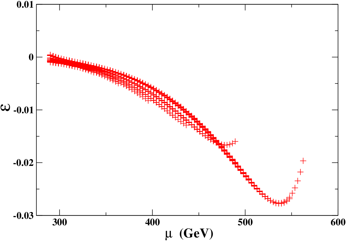
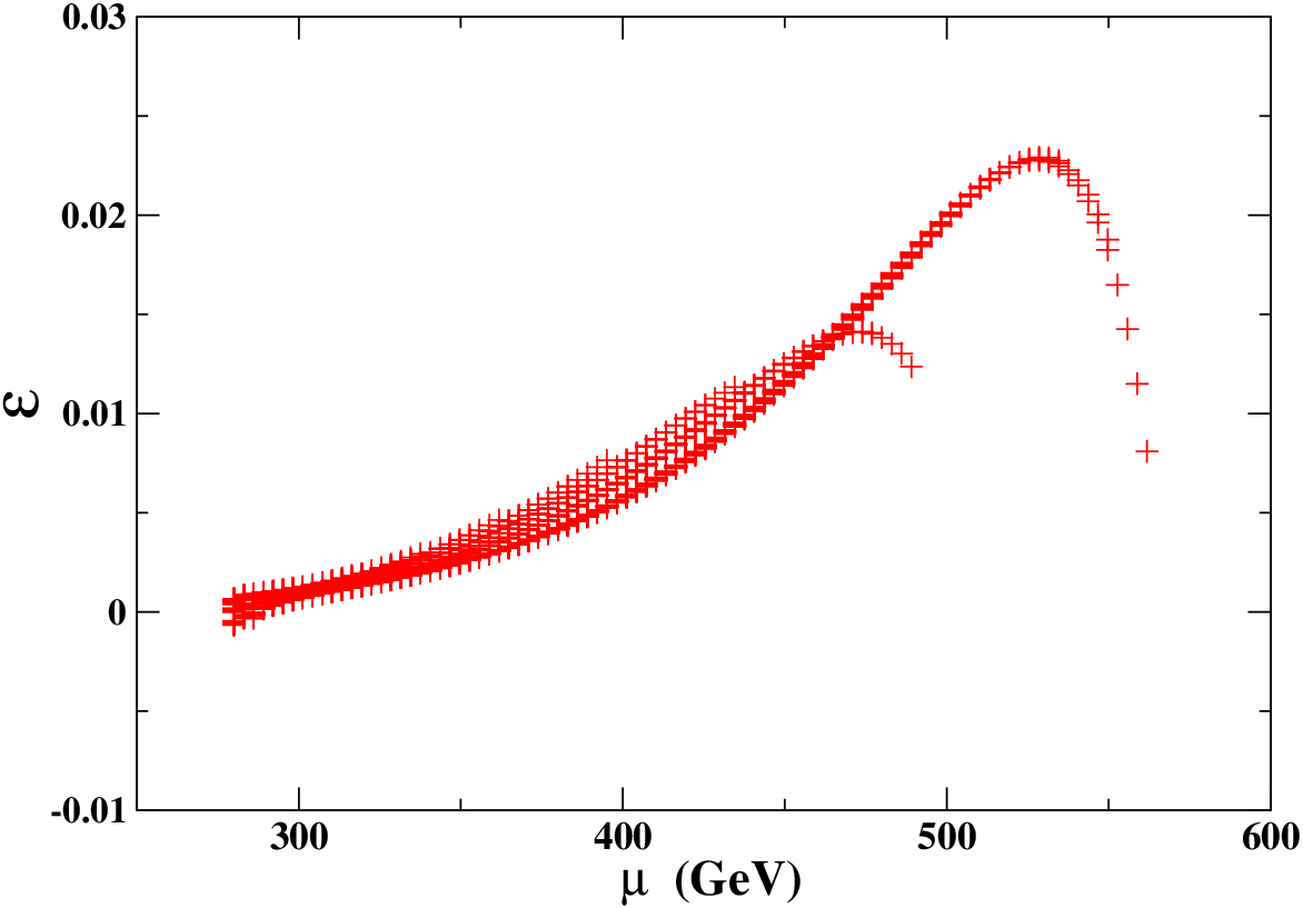
Figure 8: ε\varepsilon as a function of μ\mu. We fix λ=0.4\lambda=0.4 and κ=0.5\kappa=0.5. M1=66​G​e​VM_{1}=66GeV, M2=133​G​e​VM_{2}=133GeV and M3=500​G​e​VM_{3}=500GeV. The figure on the left represents the normal supersymmetric hierarchy (mτ~=300​G​e​Vm_{\tilde{\tau}}=300GeV and mμ~=200​G​e​Vm_{\tilde{\mu}}=200GeV), the figure on the right represents the inverted supersymmetric hierarchy (mτ~=200​G​e​Vm_{\tilde{\tau}}=200GeV and mμ~=300​G​e​Vm_{\tilde{\mu}}=300GeV).

We consider two experimentally allowed cases for the sleptons with a splitting between the third and the second generation:

  • .

    mτ~=300​G​e​Vm_{\tilde{\tau}}=300GeV and mμ~=200​G​e​Vm_{\tilde{\mu}}=200GeV (normal supersymmetric hierarchy)

  • .

    mτ~=200​G​e​Vm_{\tilde{\tau}}=200GeV and mμ~=300​G​e​Vm_{\tilde{\mu}}=300GeV (inverted supersymmetric hierarchy)

We also assume that squarks are much heavier than sleptons: MQ~=1​T​e​VM_{\tilde{Q}}=1TeV. These are the effects of gluino masses in the renormalization group evolution of scalar masses.

The splitting among the sleptons of the second and third generations is mainly responsible for the size of Δ​ρ\Delta\rho.

Refer to caption  Refer to caption

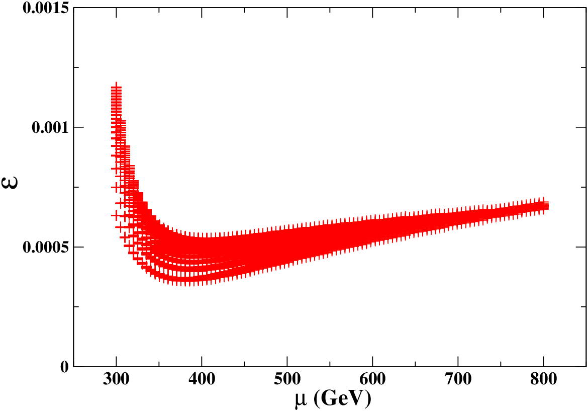
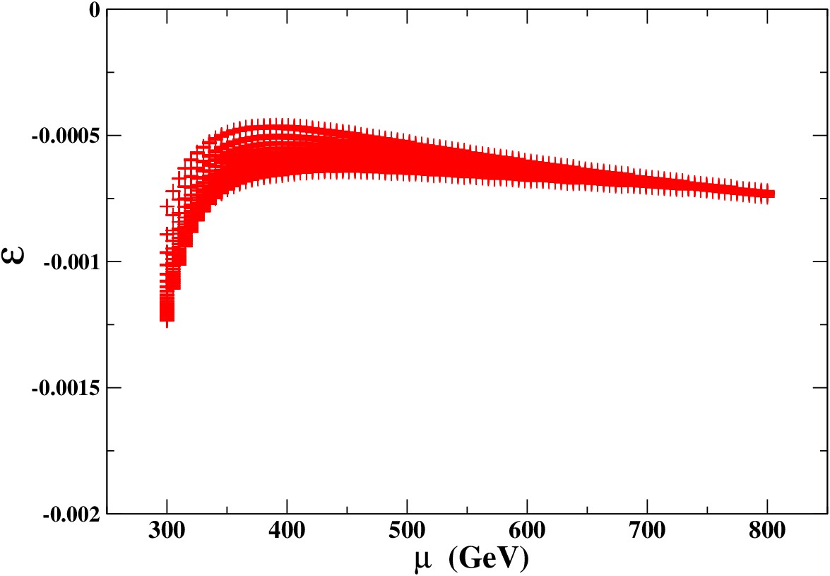
Figure 9: ε\varepsilon as a function of μ\mu. We fix λ=0.4\lambda=0.4 and κ=0.5\kappa=0.5. M1=150​G​e​VM_{1}=150GeV, M2=300​G​e​VM_{2}=300GeV and M3=1​T​e​VM_{3}=1TeV. The figure on the left represents the normal supersymmetric hierarchy, the figure on the right represents the inverted supersymmetric hierarchy.

The purpose of this Section is the investigation of the supersymmetric parameter space in some specific cases. To this end we made a subroutine to the Fortran code NMHDECAY, which is available on the NMSSMTools web page [40], [44], [45]. This subroutine computes the different R-parity conserved supersymmetric contributions to ε\varepsilon. Note that ε\varepsilon is the same for antineutrinos, as in the SM.

By making scans over the supersymmetric parameter space, we can obtain, in some regions of the parameter space, divergences for either mχj+=mτ~km_{\chi_{j}^{+}}=m_{\tilde{\tau}_{k}}, mχj+=mμ~Lm_{\chi_{j}^{+}}=m_{\tilde{\mu}_{L}} or mχi0=mν~ℓm_{\chi_{i}^{0}}=m_{\tilde{\nu}_{\ell}}. This is because we assume vanishing external legs.

In supersymmetry, there are many parameters. ε\varepsilon doesn’t depend very much on λ\lambda and κ\kappa so we fix them as we usually do in supersymmetry: λ=0.4\lambda=0.4 and κ=0.5\kappa=0.5 . We allow some other parameters to vary: tan​β{\rm tan}\beta, MAM_{A} and μeff\mu_{\rm eff}.

tan​β{\rm tan}\beta is the ratio vu/vdv_{u}/v_{d} where vuv_{u} and vdv_{d} are the v.e.v. of the scalar Higgs fields HuH_{u} and HdH_{d}. MAM_{A} is an effective supersymmetric parameter somewhat equivalent to the second pseudoscalar Higgs mass in our regions of the parameter space.


We show two different illustrative situations motivated by high-energy models for the gaugino masses:

  • .

    M1=66​G​e​VM_{1}=66GeV, M2=133​G​e​VM_{2}=133GeV and M3=500​G​e​VM_{3}=500GeV (cf Fig.(8))

  • .

    M1=150​G​e​VM_{1}=150GeV, M2=300​G​e​VM_{2}=300GeV and M3=1​T​e​VM_{3}=1TeV (cf Fig.(9))

In Fig.(8), tan​β{\rm tan}\beta varies between 2 and 15, MAM_{A} varies between 579 and 2000 GeV, μ\mu varies between 300 and 800 GeV. We see in Fig.(8) that contrary to the SM case, Vμ​τV_{\mu\tau} can be either positive or negative.

In Fig.(9), tan​β{\rm tan}\beta varies between 2 and 18 (for the figure on the left) and between 2 and 9.6 (for the figure on the right), MAM_{A} varies between 500 and 1000 GeV, μ\mu varies between 200 and 564 GeV.

On the other hand, as we can see in the Fig.(9), ε\varepsilon can go up to 2× 10−22\times\,10^{-2} in this region of the parameter space. The sign of μ\mu does not have an important impact on the maximal value that ε\varepsilon can reach.

We finally mention that other extensions of the SM may also lead to sizable effects upon Δ​nτ​μ\Delta n_{\tau\mu}. In the next section, we will consider supersymmetric RR-parity violating interactions which can have important effects on the neutrino indices of refraction already at the tree-level [46].

IV R-parity breaking SUSY corrections

IV.1 Introduction

The superpotential W𝑁𝑀𝑆𝑆𝑀\it{W}_{NMSSM} is not the most general superpotential we wan write because there exist some other gauge invariant couplings that we didn’t take into account. These new couplings break a discrete symmetry called R-parity. This symmetry requires that an interaction must have an even number of SUSY particles. If R-parity is broken, the LSP will no longer be stable [47]. R-parity violating interactions also violate lepton number (L\it{L}) or baryon number (B\it{B}). To be as general as possible, the superpotential has to contain the following terms:

WR̸P=∑i,j,k(12​λ𝑖𝑗𝑘​L^i​L^j​E^kc+λ𝑖𝑗𝑘′​L^i​Q^j​D^kc+12​λ𝑖𝑗𝑘′′​εα​β​γ​U^ic​α​D^jc​β​D^kc​γ+μi​H^u​L^i+λi​S^​H^u​L^i)\displaystyle\it{W}_{\not{R}_{P}}=\sum_{i,j,k}\left(\frac{1}{2}\lambda_{ijk}\hat{L}_{i}\hat{L}_{j}\hat{E}_{k}^{c}+\lambda^{\prime}_{ijk}\hat{L}_{i}\hat{Q}_{j}\hat{D}_{k}^{c}+\frac{1}{2}\lambda^{\prime\prime}_{ijk}\varepsilon_{\alpha\beta\gamma}\hat{U}_{i}^{c\alpha}\hat{D}_{j}^{c\beta}\hat{D}_{k}^{c\gamma}+\mu_{i}\hat{H}_{u}\hat{L}_{i}+\lambda_{i}\hat{S}\hat{H}_{u}\hat{L}_{i}\right) (28)

The lagrangian ℒR̸P{\cal{L}}_{\not{R}_{P}} can be derived using the common procedure [48, 37].

If we consider this part of the superpotential:

W𝑚𝑎𝑠𝑠𝑒𝑠=W𝑁𝑀𝑆𝑆𝑀+μi​H^u​L^i+λi​S^​H^u​L^i\displaystyle\it{W}_{masses}=\it{W}_{NMSSM}+\mu_{i}\hat{H}_{u}\hat{L}_{i}+\lambda_{i}\hat{S}\hat{H}_{u}\hat{L}_{i} (29)

we can generate two neutrino masses at tree-level [37] by mixing neutrinos and neutralinos. By considering a See-Saw-like mechanism, the mass matrix is:

ℳχ0~=(ℳN​M​S​S​MξR̸PTξR̸P03×3)\displaystyle{\cal{M}}_{\tilde{\chi^{0}}}=\left(\begin{array}[]{cc}{\cal{M}}_{NMSSM}&\xi_{\not{R}_{P}}^{T}\cr\xi_{\not{R}_{P}}&0_{3\times 3}\end{array}\right)

where ℳN​M​S​S​M{\cal{M}}_{NMSSM} is the R-parity conserved neutralino mass matrix and ξR̸P\xi_{\not{R}_{P}} is the part of the mass matrix induced by R-parity violation which mix neutralinos and neutrinos. We will assume here: vi/vu,d≪1v_{i}/v_{u,d}\ll 1, |μi/μ|≪1|\mu_{i}/\mu|\ll 1 and |λi/λ|≪1|\lambda_{i}/\lambda|\ll 1 in order to reproduce the neutrino phenomenology. viv_{i} are the v.e.v. of the sneutrinos.
This model is self-consistent because we give here a way to generate the neutrino masses contrary to many other scenarios of radiative corrections on neutrino indices of refraction.

In the following, νi=Ni​j​Ψ~j\nu_{i}=N_{ij}\tilde{\Psi}_{j} where Ψ~T=(B~,W~3,h~u,h~d,s~,νe,νμ,ντ)\tilde{\Psi}^{T}=(\tilde{B},\tilde{W}_{3},\tilde{h}_{u},\tilde{h}_{d},\tilde{s},\nu_{e},\nu_{\mu},\nu_{\tau}), i=1..3i=1..3 and j=1..8j=1..8. νe\nu_{e}, νμ\nu_{\mu} and ντ\nu_{\tau} represent the neutrinos in their flavour basis, νi\nu_{i} represent the neutrinos in their mass basis. χi0=N(i+3)​j​Ψ~j\chi^{0}_{i}=N_{(i+3)j}\tilde{\Psi}_{j} where i=1..5i=1..5 and j=1..8j=1..8. χi0\chi^{0}_{i} are the five NMSSM’s neutralinos.

IV.2 Tree-level corrections

Because of R-parity breaking, new interactions are possible between SUSY particles. This yields new one-loop corrections but also tree level corrections contrary to the R-parity conserved case. Such tree level corrections in the Supernova context have been partially studied in [49, 46]. Since this work focuses on Vμ​τV_{\mu\tau}, we only concentrate on graphs involving μ\mu and τ\tau neutrinos. Moreover, we only consider neutrinos which do not change of flavour after the R-parity breaking interaction, therefore we are not concerned by off-diagonal term in the matter Hamiltonian.

Refer to caption

Figure 10: R-parity broken Tree-level corrections.

Here, we give a specific contribution to antineutrino scattering (Fig.10a) with left sleptons ℓ~L,i\tilde{\ell}_{L,i}:

Δρa(ℓ~L,i)=−∑i=13(λ3​i​12−λ2​i​12)g2MW2mℓ~L,i2\Delta\rho_{a}(\tilde{\ell}_{L,i})=-\sum_{i=1}^{3}\frac{(\lambda_{3i1}^{2}-\lambda_{2i1}^{2})}{g^{2}}\frac{M_{W}^{2}}{m_{\tilde{\ell}_{L,i}}^{2}} (33)

With left down squarks d~L,i\tilde{d}_{L,i} (Fig.10b):

Δρb(d~L,i)=Δρa(ℓ~L,i)(λk​i​1→λk​i​1′,ℓ~L,i→d~L,i)\Delta\rho_{b}(\tilde{d}_{L,i})=\Delta\rho_{a}(\tilde{\ell}_{L,i})\ (\lambda_{ki1}\rightarrow\lambda_{ki1}^{\prime},\tilde{\ell}_{L,i}\rightarrow\tilde{d}_{L,i}) (34)

The right sleptons ℓ~R,i\tilde{\ell}_{R,i} and the right down squarks d~R,i\tilde{d}_{R,i} do not contribute.

The following contributions induce corrections to both neutrino and antineutrino scattering:

for diagram (Fig.10c):

Δρc(χ0)=−∑j,k=15(N(j+3)​8N(i+3)​8−N(j+3)​7N(i+3)​7)(N(j+3)​4N(i+3)​4−N(j+3)​3N(i+3)​3)\displaystyle\Delta\rho_{c}(\chi^{0})=-\sum_{j,k=1}^{5}\left(N_{(j+3)8}N_{(i+3)8}-N_{(j+3)7}N_{(i+3)7}\right)\left(N_{(j+3)4}N_{(i+3)4}-N_{(j+3)3}N_{(i+3)3}\right) (35)

for diagram (Fig.10d):

Δ​ρd​(ℓ~L,i)=Δ​ρa​(ℓ~L,i)\Delta\rho_{d}(\tilde{\ell}_{L,i})=\Delta\rho_{a}(\tilde{\ell}_{L,i}) (36)

for diagram (Fig.10e):

Δ​ρe​(d~L,i)=Δ​ρb​(d~L,i)\Delta\rho_{e}(\tilde{d}_{L,i})=\Delta\rho_{b}(\tilde{d}_{L,i}) (37)

For (Fig.10d) and (Fig.10e), the right sleptons ℓ~R,i\tilde{\ell}_{R,i} and the right down squarks d~R,i\tilde{d}_{R,i} do not contribute.

IV.3 Self-energy corrections

We willingly leave certain factors not simplified to be able to compare with other corrections more rapidly. All the contributions will be equal for neutrino and antineutrino scattering.

Refer to caption

Figure 11: R-parity broken Self-energy corrections.

For Fig.(11f):

Δρℓ~R(Σ)=−αW8​π∑i,j=13(λ3​i​j2−λ2​i​j2)g2{G0(Xℓi​ℓ~R,j,1)+lnmℓ~R,j2μ2},\displaystyle\Delta\rho^{\tilde{\ell}_{R}}(\Sigma)=-{\alpha_{W}\over 8\pi}\sum_{i,j=1}^{3}\frac{(\lambda_{3ij}^{2}-\lambda_{2ij}^{2})}{g^{2}}\left\{G_{0}(X_{\ell_{i}\tilde{\ell}_{R,j}},1)+{\rm ln}{m_{\tilde{\ell}_{R,j}}^{2}\over\mu^{2}}\right\}, (38)
Δρd~R(Σ)=Δρℓ~R(Σ)(λk​i​j→λk​i​j′,ℓ~R,j→d~R,j)\Delta\rho^{\tilde{d}_{R}}(\Sigma)=\Delta\rho^{\tilde{\ell}_{R}}(\Sigma)\ (\lambda_{kij}\rightarrow\lambda_{kij}^{\prime},\tilde{\ell}_{R,j}\rightarrow\tilde{d}_{R,j})

For Fig.(11h):

Δρℓ~L(Σ)=Δρℓ~R(Σ)(λk​i​j→λk​j​i,ℓ~R,j→ℓ~L,j),\displaystyle\Delta\rho^{\tilde{\ell}_{L}}(\Sigma)=\Delta\rho^{\tilde{\ell}_{R}}(\Sigma)\ (\lambda_{kij}\rightarrow\lambda_{kji},\tilde{\ell}_{R,j}\rightarrow\tilde{\ell}_{L,j}), (39)
Δρd~L(Σ)=Δρℓ~R(Σ)(λk​i​j→λk​j​i′,ℓ~R,j→d~L,j)\Delta\rho^{\tilde{d}_{L}}(\Sigma)=\Delta\rho^{\tilde{\ell}_{R}}(\Sigma)\ (\lambda_{kij}\rightarrow\lambda_{kji}^{\prime},\tilde{\ell}_{R,j}\rightarrow\tilde{d}_{L,j})

In the R-parity breaking scenario, there are NMSSM specific self-energies due to the term λi​S^​H^u​L^i\lambda_{i}\hat{S}\hat{H}_{u}\hat{L}_{i} in the superpotential. This term induce one new coupling between a neutrino, one Higgs (scalar or pseudoscalar) and a neutralino. We present here the contributions for scalar Higgses and for pseudoscalar Higgses.

For both Fig.(11g) and (11i), the contribution from scalar higgses:

Δρh(Σ)=−αW8​π(λ32−λ22)g2∑i=15∑j=13(N(i+3)​52Sj​12+N(i+3)​32Sj​32){G0(Xχi0​hj,1)+lnmhj2μ2}\displaystyle\Delta\rho^{h}(\Sigma)=-{\alpha_{W}\over 8\pi}\frac{(\lambda_{3}^{2}-\lambda_{2}^{2})}{g^{2}}\sum_{i=1}^{5}\sum_{j=1}^{3}(N_{(i+3)5}^{2}S_{j1}^{2}+N_{(i+3)3}^{2}S_{j3}^{2})\left\{G_{0}(X_{\chi^{0}_{i}h_{j}},1)+{\rm ln}{m_{h_{j}}^{2}\over\mu^{2}}\right\} (40)

from pseudoscalar higgses:

Δρa(Σ)=−αW8​π(λ32−λ22)g2∑i=15∑j=12(N(i+3)​52Pj​12+N(i+3)​32Pj​32){G0(Xχi0​aj,1)+lnmaj2μ2}\displaystyle\Delta\rho^{a}(\Sigma)=-{\alpha_{W}\over 8\pi}\frac{(\lambda_{3}^{2}-\lambda_{2}^{2})}{g^{2}}\sum_{i=1}^{5}\sum_{j=1}^{2}(N_{(i+3)5}^{2}P_{j1}^{2}+N_{(i+3)3}^{2}P_{j3}^{2})\left\{G_{0}(X_{\chi^{0}_{i}a_{j}},1)+{\rm ln}{m_{a_{j}}^{2}\over\mu^{2}}\right\} (41)

IV.4 penguin type diagrams

Refer to caption

Figure 12: R-parity broken penguin type diagrams.

We consider here the penguin diagrams. All the contributions will be equal for neutrino and antineutrino scattering.

For the diagram of Fig.(13j) and Fig.(13l):

ΔρPℓ~L(ℓ)=−αW16​π∑i,j=13(λ3​j​i2−λ2​j​i2)g2[G0(Xℓ~L,j,ℓi,1)+ln(mℓi2μ2)],\Delta\rho_{P}^{\tilde{\ell}_{L}}(\ell)=-\frac{\alpha_{W}}{16\pi}\sum_{i,j=1}^{3}\frac{(\lambda^{2}_{3ji}-\lambda^{2}_{2ji})}{g^{2}}\left[G_{0}(X_{\tilde{\ell}_{L,j},\ell_{i}},1)+\ln(\frac{m^{2}_{{\ell}_{i}}}{\mu^{2}})\right], (42)
ΔρPd~L(d)=ΔρPℓ~L(ℓ)(λk​j​i→λk​j​i′,ℓ~L,j→d~L,j,ℓi→di)\Delta\rho_{P}^{\tilde{d}_{L}}(d)=\Delta\rho_{P}^{\tilde{\ell}_{L}}(\ell)\ (\lambda_{kji}\rightarrow\lambda_{kji}^{\prime},\tilde{\ell}_{L,j}\rightarrow\tilde{d}_{L,j},\ell_{i}\rightarrow d_{i})

For the diagram of Fig.(13k) and Fig.(13m):

ΔρPℓ(ℓ~L)=−αW4​πcLℓ∑i,j=13(λ3​j​i2−λ2​j​i2)g2[G0(Xℓi,ℓ~L,j,1)+ln(mℓ~L,j2μ2)]\Delta\rho_{P}^{\ell}(\tilde{\ell}_{L})=-\frac{\alpha_{W}}{4\pi}c^{\ell}_{L}\sum_{i,j=1}^{3}\frac{(\lambda^{2}_{3ji}-\lambda^{2}_{2ji})}{g^{2}}\left[G_{0}(X_{\ell_{i},\tilde{\ell}_{L,j}},1)+\ln(\frac{m^{2}_{\tilde{\ell}_{L,j}}}{\mu^{2}})\right] (43)
ΔρPd(d~L)=ΔρPℓ(ℓ~L)(λk​j​i→λk​j​i′,ℓ~L,j→d~L,j,ℓi→di)\Delta\rho_{P}^{d}(\tilde{d}_{L})=\Delta\rho_{P}^{\ell}(\tilde{\ell}_{L})\ (\lambda_{kji}\rightarrow\lambda_{kji}^{\prime},\tilde{\ell}_{L,j}\rightarrow\tilde{d}_{L,j},\ell_{i}\rightarrow d_{i})

For all the previous penguin diagrams, the right sleptons ℓ~R,j\tilde{\ell}_{R,j} and the right squarks d~R,j\tilde{d}_{R,j} do not contribute.

We have below NMSSM specific penguins also due to the term λi​S^​H^u​L^i\lambda_{i}\hat{S}\hat{H}_{u}\hat{L}_{i} in the superpotential.

Refer to caption

Figure 13: R-parity broken NMSSM specific penguin type diagrams.

For the diagram of Fig.(13p):

Δ​ρph​(χ0)=−αW8​πλ32−λ22g2∑i,j=15∑m=13N(i+3)​5N(j+3)​5Sm​12(N(j+3)​4N(i+3)​4−N(j+3)​3N(i+3)​3)×[2​H0​(Xχi0​hm,Xχj0​hm)+{G0​(Xχi0​hm,Xχj0​hm)+ln​mhm2μ2}],\begin{array}[]{rcl}\Delta\rho^{h}_{p}(\chi^{0})&=&-{\alpha_{W}\over 8\pi}\frac{\lambda_{3}^{2}-\lambda_{2}^{2}}{g^{2}}\sum_{i,j=1}^{5}\sum_{m=1}^{3}N_{(i+3)5}N_{(j+3)5}S_{m1}^{2}\left(N_{(j+3)4}N_{(i+3)4}-N_{(j+3)3}N_{(i+3)3}\right)\\ &&\times\left[2H_{0}(X_{\chi^{0}_{i}h_{m}},X_{\chi^{0}_{j}h_{m}})+\left\{G_{0}(X_{\chi^{0}_{i}h_{m}},X_{\chi^{0}_{j}h_{m}})+{\rm ln}{m_{h_{m}}^{2}\over\mu^{2}}\right\}\right],\end{array} (44)

For the diagram of Fig.(13n):

Δ​ρpa​(χ0)=−αW8​πλ32−λ22g2∑i,j=15∑n=12N(i+3)​5N(j+3)​5Pn​12(N(j+3)​4N(i+3)​4−N(j+3)​3N(i+3)​3)×[2​H0​(Xχi0​an,Xχj0​an)+{G0​(Xχi0​an,Xχj0​an)+ln​man2μ2}],\begin{array}[]{rcl}\Delta\rho^{a}_{p}(\chi^{0})&=&-{\alpha_{W}\over 8\pi}\frac{\lambda_{3}^{2}-\lambda_{2}^{2}}{g^{2}}\sum_{i,j=1}^{5}\sum_{n=1}^{2}N_{(i+3)5}N_{(j+3)5}P_{n1}^{2}\left(N_{(j+3)4}N_{(i+3)4}-N_{(j+3)3}N_{(i+3)3}\right)\\ &&\times\left[2H_{0}(X_{\chi^{0}_{i}a_{n}},X_{\chi^{0}_{j}a_{n}})+\left\{G_{0}(X_{\chi^{0}_{i}a_{n}},X_{\chi^{0}_{j}a_{n}})+{\rm ln}{m_{a_{n}}^{2}\over\mu^{2}}\right\}\right],\end{array} (45)

We have two identical contributions from the diagram of Fig.(13o) and Fig.(13q) and we obtain:

Δρpχ0=−αW4​πλ32−λ22g2∑i=15∑m=13∑n=12N(i+3)​52Sm​1Pn​1AMm​n{G0(Xhm​χi0,Xan​χi0)+lnmχi02μ2}\displaystyle\Delta\rho^{\chi^{0}}_{p}=-{\alpha_{W}\over 4\pi}\frac{\lambda_{3}^{2}-\lambda_{2}^{2}}{g^{2}}\sum_{i=1}^{5}\sum_{m=1}^{3}\sum_{n=1}^{2}N_{(i+3)5}^{2}S_{m1}P_{n1}A^{mn}_{M}\left\{G_{0}(X_{h_{m}\chi^{0}_{i}},X_{a_{n}\chi^{0}_{i}})+{\rm ln}{m_{\chi^{0}_{i}}^{2}\over\mu^{2}}\right\} (46)

where AMm​n=Sm​1​Pn​1−Sm​2​Pn​2A^{mn}_{\it{M}}=S_{m1}P_{n1}-S_{m2}P_{n2} following the notation of [40].

IV.5 Box diagrams

IV.5.1 R-parity broken box diagrams

Refer to caption  Refer to caption

Figure 14: R-parity broken box diagrams.

We present in this section the box diagrams corrections. Each box diagram correction involves Fierz transformations to obtain a similar form as the SM tree level interaction. The box diagrams with crossed fermions lines (Fig.14q2, Fig.14r2, Fig.14s2, Fig.14u2, Fig.14v2, Fig.14w2) will only contribute to neurinos, meanwhile the uncrossed fermion lines (Fig.14q1, Fig.14r1, Fig.14s1, Fig.14u1, Fig.14v1, Fig.14w1) will contribute to antineutrinos. However, the contributions to antineutrino scattering will be exactly the same as the contributions to neutrino scattering. We show below the contributions to neutrino scattering.

For the diagram of Fig.(14v2) with ℓ~L,i−d~R,m\tilde{\ell}_{L,i}-\tilde{d}_{R,m}:

Δρb​o​xv​2(ℓ~L−d~R)=−αW8​π∑i,j,k,m=13MW2md~R,m2(λ3​i​j​λ3​i​k−λ2​i​j​λ2​i​k)​λj​1​m′​λk​1​m′g4G′(Xℓj,d~R,m,Xℓk,d~R,m,Xℓ~L,i,d~R,m).\Delta\rho_{box}^{v2}(\tilde{\ell}_{L}-\tilde{d}_{R})=-\frac{\alpha_{W}}{8\pi}\sum_{i,j,k,m=1}^{3}\frac{M^{2}_{W}}{m^{2}_{\tilde{d}_{R,m}}}\frac{(\lambda_{3ij}\lambda_{3ik}-\lambda_{2ij}\lambda_{2ik})\lambda^{\prime}_{j1m}\lambda^{\prime}_{k1m}}{g^{4}}G^{\prime}(X_{\ell_{j},\tilde{d}_{R,m}},X_{\ell_{k},\tilde{d}_{R,m}},X_{\tilde{\ell}_{L,i},\tilde{d}_{R,m}}). (47)

For the diagram of Fig.(14r2) with d~L,i−ℓ~L,m\tilde{d}_{L,i}-\tilde{\ell}_{L,m} and the diagram of Fig.(14s2) with d~L,i−u~L,m\tilde{d}_{L,i}-\tilde{u}_{L,m}:

Δρb​o​xr​2(d~L−ℓ~L)=Δρb​o​xv​2(ℓ~L−d~R)(λ→λ′,λj​1​m′λk​1​m′→λm​1​j′λm​1​k′,lj,k→dj,k,d~R,m→ℓ~L,m),\Delta\rho_{box}^{r2}(\tilde{d}_{L}-\tilde{\ell}_{L})=\Delta\rho_{box}^{v2}(\tilde{\ell}_{L}-\tilde{d}_{R})\ (\lambda\rightarrow\lambda^{\prime},\lambda^{\prime}_{j1m}\lambda^{\prime}_{k1m}\rightarrow\lambda^{\prime}_{m1j}\lambda^{\prime}_{m1k},l_{j,k}\rightarrow d_{j,k},\tilde{d}_{R,m}\rightarrow\tilde{\ell}_{L,m}), (48)
Δρb​o​xs​2(d~L−u~L)=Δρb​o​xr​2(d~L−ℓ~L)(λm​1​j′λm​1​k′→λ1​m​j′λ1​m​k′,ℓ~L,m→u~L,m).\Delta\rho_{box}^{s2}(\tilde{d}_{L}-\tilde{u}_{L})=\Delta\rho_{box}^{r2}(\tilde{d}_{L}-\tilde{\ell}_{L})\ (\lambda^{\prime}_{m1j}\lambda^{\prime}_{m1k}\rightarrow\lambda^{\prime}_{1mj}\lambda^{\prime}_{1mk},\tilde{\ell}_{L,m}\rightarrow\tilde{u}_{L,m}).

For the diagram of Fig.(14r2) with d~R,i−ℓ~L,m\tilde{d}_{R,i}-\tilde{\ell}_{L,m} and the diagram of Fig.(14s2) with d~R,i−u~L,m\tilde{d}_{R,i}-\tilde{u}_{L,m}:

Δ​ρb​o​xr​2​(d~R−ℓ~L)=αW4​π​∑i,j,k,m=13MW2mℓ~L,m2​(λ3​j​i′​λ3​k​i′−λ2​j​i′​λ2​k​i′)​λm​1​j′​λm​1​k′g4​H′​(Xdj,ℓ~L,m,Xdk,ℓ~L,m,Xd~R,i,ℓ~L,m),\Delta\rho_{box}^{r2}(\tilde{d}_{R}-\tilde{\ell}_{L})=\frac{\alpha_{W}}{4\pi}\sum_{i,j,k,m=1}^{3}\frac{M^{2}_{W}}{m^{2}_{\tilde{\ell}_{L,m}}}\frac{(\lambda^{\prime}_{3ji}\lambda^{\prime}_{3ki}-\lambda^{\prime}_{2ji}\lambda^{\prime}_{2ki})\lambda^{\prime}_{m1j}\lambda^{\prime}_{m1k}}{g^{4}}H^{\prime}(X_{d_{j},\tilde{\ell}_{L,m}},X_{d_{k},\tilde{\ell}_{L,m}},X_{\tilde{d}_{R,i},\tilde{\ell}_{L,m}}), (49)
Δρb​o​xs​2(d~R−u~L)=Δρb​o​xr​2(d~R−ℓ~L)(λm​1​j′λm​1​k′→λ1​m​j′λ1​m​k′,ℓ~L,m→u~L,m).\Delta\rho_{box}^{s2}(\tilde{d}_{R}-\tilde{u}_{L})=\Delta\rho_{box}^{r2}(\tilde{d}_{R}-\tilde{\ell}_{L})\ (\lambda^{\prime}_{m1j}\lambda^{\prime}_{m1k}\rightarrow\lambda^{\prime}_{1mj}\lambda^{\prime}_{1mk},\tilde{\ell}_{L,m}\rightarrow\tilde{u}_{L,m}).

For the diagram of Fig.(14q2) with d~R,i−ν~L,m\tilde{d}_{R,i}-\tilde{\nu}_{L,m} and for the diagram of Fig.(14u2) with ℓ~R,i−ν~L,m\tilde{\ell}_{R,i}-\tilde{\nu}_{L,m}:

Δ​ρb​o​xq​2​(d~R−ν~L)=αW4​π​∑i,j,k,m=13MW2mν~L,m2​(λ3​i​j′​λ3​i​k′−λ2​i​j′​λ2​i​k′)​λm​j​1′​λm​k​1′g4​H′​(Xdj,ν~L,m,Xdk,ν~L,m,Xd~R,i,ν~L,m),\Delta\rho_{box}^{q2}(\tilde{d}_{R}-\tilde{\nu}_{L})=\frac{\alpha_{W}}{4\pi}\sum_{i,j,k,m=1}^{3}\frac{M^{2}_{W}}{m^{2}_{\tilde{\nu}_{L,m}}}\frac{(\lambda^{\prime}_{3ij}\lambda^{\prime}_{3ik}-\lambda^{\prime}_{2ij}\lambda^{\prime}_{2ik})\lambda^{\prime}_{mj1}\lambda^{\prime}_{mk1}}{g^{4}}H^{\prime}(X_{d_{j},\tilde{\nu}_{L,m}},X_{d_{k},\tilde{\nu}_{L,m}},X_{\tilde{d}_{R,i},\tilde{\nu}_{L,m}}), (50)
Δρb​o​xu​2(ℓ~R−ν~L)=Δρb​o​xq​2(d~R−ν~L)(λm​j​1′λm​k​1′→λm​1​j′λm​1​k′thenλ′→λ,dj,k→ℓj,k,d~R,i→ℓ~R,i).\Delta\rho_{box}^{u2}(\tilde{\ell}_{R}-\tilde{\nu}_{L})=\Delta\rho_{box}^{q2}(\tilde{d}_{R}-\tilde{\nu}_{L})\ (\lambda^{\prime}_{mj1}\lambda^{\prime}_{mk1}\rightarrow\lambda^{\prime}_{m1j}\lambda^{\prime}_{m1k}{\rm then}\lambda^{\prime}\rightarrow\lambda,d_{j,k}\rightarrow\ell_{j,k},\tilde{d}_{R,i}\rightarrow\tilde{\ell}_{R,i}).

For the diagram of Fig.(14v2) with ℓ~R,i−d~R,m\tilde{\ell}_{R,i}-\tilde{d}_{R,m} and for the diagram of Fig.(14w2) with ℓ~L,i−u~L,m\tilde{\ell}_{L,i}-\tilde{u}_{L,m}:

Δ​ρb​o​xv​2​(ℓ~R−d~R)=αW4​π​∑i,j,k,m=13MW2md~R,m2​(λ3​j​i​λ3​k​i−λ2​j​i​λ2​k​i)​λj​1​m′​λk​1​m′g4​H′​(Xℓj,d~R,m,Xℓk,d~R,m,Xℓ~R,i,d~R,m),\Delta\rho_{box}^{v2}(\tilde{\ell}_{R}-\tilde{d}_{R})=\frac{\alpha_{W}}{4\pi}\sum_{i,j,k,m=1}^{3}\frac{M^{2}_{W}}{m^{2}_{\tilde{d}_{R,m}}}\frac{(\lambda_{3ji}\lambda_{3ki}-\lambda_{2ji}\lambda_{2ki})\lambda^{\prime}_{j1m}\lambda^{\prime}_{k1m}}{g^{4}}H^{\prime}(X_{\ell_{j},\tilde{d}_{R,m}},X_{\ell_{k},\tilde{d}_{R,m}},X_{\tilde{\ell}_{R,i},\tilde{d}_{R,m}}), (51)
Δρb​o​xw​2(ℓ~L−u~L)=Δρb​o​xv​2(ℓ~R−d~R)(λj​1​m′λk​1​m′→λj​m​1′λk​m​1′,d~R,m→u~L,m,ℓ~R,i→ℓ~L,i).\Delta\rho_{box}^{w2}(\tilde{\ell}_{L}-\tilde{u}_{L})=\Delta\rho_{box}^{v2}(\tilde{\ell}_{R}-\tilde{d}_{R})\ (\lambda^{\prime}_{j1m}\lambda^{\prime}_{k1m}\rightarrow\lambda^{\prime}_{jm1}\lambda^{\prime}_{km1},\tilde{d}_{R,m}\rightarrow\tilde{u}_{L,m},\tilde{\ell}_{R,i}\rightarrow\tilde{\ell}_{L,i}).

For the diagram of Fig.(14r2) with d~L,i−d~R,m\tilde{d}_{L,i}-\tilde{d}_{R,m}:

Δ​ρb​o​x,α​σr​2​(d~L−d~R)=αW4​π​∑i,j,k,m=13∑β,δ,γ=13MW2md~R,mγ2​(λ3​i​j′​λ3​i​k′−λ2​i​j′​λ2​i​k′)​λ1​m​j′′​λ1​m​k′′g4​ϵσ​γ​δ​ϵα​γ​β​H′​(Xdjδ,d~R,mγ,Xdkβ,d~R,mγ,Xd~L,i,d~R,mγ).\Delta\rho_{box,\alpha\sigma}^{r2}(\tilde{d}_{L}-\tilde{d}_{R})=\frac{\alpha_{W}}{4\pi}\sum_{i,j,k,m=1}^{3}\sum_{\beta,\delta,\gamma=1}^{3}\frac{M^{2}_{W}}{m^{2}_{\tilde{d}^{\gamma}_{R,m}}}\frac{(\lambda^{\prime}_{3ij}\lambda^{\prime}_{3ik}-\lambda^{\prime}_{2ij}\lambda^{\prime}_{2ik})\lambda^{\prime\prime}_{1mj}\lambda^{\prime\prime}_{1mk}}{g^{4}}\epsilon_{\sigma\gamma\delta}\epsilon_{\alpha\gamma\beta}H^{\prime}(X_{d^{\delta}_{j},\tilde{d}^{\gamma}_{R,m}},X_{d^{\beta}_{k},\tilde{d}^{\gamma}_{R,m}},X_{\tilde{d}_{L,i},\tilde{d}^{\gamma}_{R,m}}). (52)

For the diagram of Fig.(14q2) with d~R,i−u~R,m\tilde{d}_{R,i}-\tilde{u}_{R,m}:

Δ​ρb​o​x,β​σq​2​(d~R−u~R)=αW16​π​∑i,j,k,m=13∑α,δ,γ=13MW2mu~R,mα2​(λ3​j​i′​λ3​k​i′−λ2​j​i′​λ2​k​i′)​λm​j​1′′​λm​k​1′′g4​ϵα​δ​σ​ϵα​γ​β​H′​(Xdjγ,u~R,mα,Xdkδ,u~R,mα,Xd~R,i,u~R,mα).\Delta\rho_{box,\beta\sigma}^{q2}(\tilde{d}_{R}-\tilde{u}_{R})=\frac{\alpha_{W}}{16\pi}\sum_{i,j,k,m=1}^{3}\sum_{\alpha,\delta,\gamma=1}^{3}\frac{M^{2}_{W}}{m^{2}_{\tilde{u}^{\alpha}_{R,m}}}\frac{(\lambda^{\prime}_{3ji}\lambda^{\prime}_{3ki}-\lambda^{\prime}_{2ji}\lambda^{\prime}_{2ki})\lambda^{\prime\prime}_{mj1}\lambda^{\prime\prime}_{mk1}}{g^{4}}\epsilon_{\alpha\delta\sigma}\epsilon_{\alpha\gamma\beta}H^{\prime}(X_{d_{j}^{\gamma},\tilde{u}^{\alpha}_{R,m}},X_{d_{k}^{\delta},\tilde{u}^{\alpha}_{R,m}},X_{\tilde{d}_{R,i},\tilde{u}^{\alpha}_{R,m}}). (53)

The indices of ϵ\epsilon denote S​U​(3)SU(3) color indices where ϵ\epsilon is antisymmetric, ϵα​β​γ=ϵβ​γ​α=ϵγ​α​β\epsilon_{\alpha\beta\gamma}=\epsilon_{\beta\gamma\alpha}=\epsilon_{\gamma\alpha\beta}. For example, for the diagram of Fig.(14q2) with d~L,i−u~R,m\tilde{d}_{L,i}-\tilde{u}_{R,m}, the down quark on the left carries the index β\beta and the down quark on the right carries the index σ\sigma:

Δ​ρb​o​x,β​σq​2​(d~L−u~R)\displaystyle\Delta\rho_{box,\beta\sigma}^{q2}(\tilde{d}_{L}-\tilde{u}_{R}) =\displaystyle= αW16​π​∑i,j,k,m=13∑α,δ,γ=13MW2mu~R,mα2​(λ3​i​j′​λ3​i​k′−λ2​i​j′​λ2​i​k′)​λm​1​j′′​λm​1​k′′g4​ϵα​σ​δ​ϵα​β​γ\displaystyle\frac{\alpha_{W}}{16\pi}\sum_{i,j,k,m=1}^{3}\sum_{\alpha,\delta,\gamma=1}^{3}\frac{M^{2}_{W}}{m^{2}_{\tilde{u}^{\alpha}_{R,m}}}\frac{(\lambda^{\prime}_{3ij}\lambda^{\prime}_{3ik}-\lambda^{\prime}_{2ij}\lambda^{\prime}_{2ik})\lambda^{\prime\prime}_{m1j}\lambda^{\prime\prime}_{m1k}}{g^{4}}\epsilon_{\alpha\sigma\delta}\epsilon_{\alpha\beta\gamma} (54)
[H′​(Xdjδ,u~R,mα,Xdkγ,u~R,mα,Xd~L,i,u~R,mα)−G′​(Xdjδ,u~R,mα,Xdkγ,u~R,mα,Xd~L,i,u~R,mα)2].\displaystyle\left[H^{\prime}(X_{d_{j}^{\delta},\tilde{u}^{\alpha}_{R,m}},X_{d_{k}^{\gamma},\tilde{u}^{\alpha}_{R,m}},X_{\tilde{d}_{L,i},\tilde{u}^{\alpha}_{R,m}})-\frac{G^{\prime}(X_{d_{j}^{\delta},\tilde{u}^{\alpha}_{R,m}},X_{d_{k}^{\gamma},\tilde{u}^{\alpha}_{R,m}},X_{\tilde{d}_{L,i},\tilde{u}^{\alpha}_{R,m}})}{2}\right].

The diagram of Fig.(14q2) with d~L,i−ν~L,m\tilde{d}_{L,i}-\tilde{\nu}_{L,m} can be deducted from the previous one by removing the ϵ\epsilon factors and by taking a factor 4 and λ′′→λ′\lambda^{\prime\prime}\rightarrow\lambda^{\prime}, u~R→ν~L\tilde{u}_{R}\rightarrow\tilde{\nu}_{L}:

Δ​ρb​o​xq​2​(d~L−ν~L)\displaystyle\Delta\rho_{box}^{q2}(\tilde{d}_{L}-\tilde{\nu}_{L}) =\displaystyle= αW4​π​∑i,j,k,m=13MW2mν~L,m2​(λ3​i​j′​λ3​i​k′−λ2​i​j′​λ2​i​k′)​λm​j​1′​λm​k​1′g4\displaystyle\frac{\alpha_{W}}{4\pi}\sum_{i,j,k,m=1}^{3}\frac{M^{2}_{W}}{m^{2}_{\tilde{\nu}_{L,m}}}\frac{(\lambda^{\prime}_{3ij}\lambda^{\prime}_{3ik}-\lambda^{\prime}_{2ij}\lambda^{\prime}_{2ik})\lambda^{\prime}_{mj1}\lambda^{\prime}_{mk1}}{g^{4}} (55)
[H′​(Xdj,ν~L,m,Xdk,ν~L,m,Xd~L,i,ν~L,m)−G′​(Xdj,ν~L,m,Xdk,ν~L,m,Xd~L,i,ν~L,m)2].\displaystyle\left[H^{\prime}(X_{d_{j},\tilde{\nu}_{L,m}},X_{d_{k},\tilde{\nu}_{L,m}},X_{\tilde{d}_{L,i},\tilde{\nu}_{L,m}})-\frac{G^{\prime}(X_{d_{j},\tilde{\nu}_{L,m}},X_{d_{k},\tilde{\nu}_{L,m}},X_{\tilde{d}_{L,i},\tilde{\nu}_{L,m}})}{2}\right].

Finally, for the diagram of Fig.(14u2) with ℓ~L,i−ν~L,m\tilde{\ell}_{L,i}-\tilde{\nu}_{L,m}:

Δρb​o​xu​2(ℓ~L−ν~L)=Δρb​o​xq​2(d~L−ν~L)(λ′→λ,dj,k→ℓj,k,d~L,i→ℓ~L,i).\displaystyle\Delta\rho_{box}^{u2}(\tilde{\ell}_{L}-\tilde{\nu}_{L})=\Delta\rho_{box}^{q2}(\tilde{d}_{L}-\tilde{\nu}_{L})\ (\lambda^{\prime}\rightarrow\lambda,d_{j,k}\rightarrow\ell_{j,k},\tilde{d}_{L,i}\rightarrow\tilde{\ell}_{L,i}). (56)

The rest of diagrams do not contribute because of a different form as the correct tree level SM form given in Eq.(2).

IV.5.2 Cancelling diagrams

Refer to caption  Refer to caption

Figure 15: R-parity broken radiative corrections which cancel out. The Feynman graphs with uncrossed scalar lines on the left cancel with the Feynman graphs with crossed scalar lines on the right.

It is interesting to notice that amongst the possible radiative corrections induced by the R-parity breaking interactions, some of them cancel. Contrary to the previous box diagrams, all box diagrams in Fig.(15) should contribute equally to neutrinos and anti-neutrinos because the fermionic lines do not link the neutrinos to the fermion present in the external leg. The particles exchanged between the two fermionic lines here are all scalar.

To understand the consequences, we write the tensorial part of the scattering amplitude of a ladder scalar line box diagram (Fig.15x1) and the corresponding crossed scalar line box diagram (Fig.15x2):

For the left diagram we have:

ℳ1\displaystyle{\cal{M}}_{1} =\displaystyle= u¯(k1)[∫d​q4(2​π)4iλ3​k​i1+γ52i⁡(q̸+mℓi)q2−mℓi2iλ3​j​i1−γ52u(p1)i(p1−q)2−mℓ~L,j2i(k1−q)2−mℓ~L,k2\displaystyle\bar{u}(k_{1})\left[\int\frac{dq^{4}}{(2\pi)^{4}}i\lambda_{3ki}\frac{1+\gamma_{5}}{2}\frac{i(\not{q}+m_{\ell_{i}})}{q^{2}-m^{2}_{\ell_{i}}}i\lambda_{3ji}\frac{1-\gamma_{5}}{2}u(p_{1})\frac{i}{(p_{1}-q)^{2}-m^{2}_{\tilde{\ell}_{L,j}}}\frac{i}{(k_{1}-q)^{2}-m^{2}_{\tilde{\ell}_{L,k}}}\right. (57)
u¯(k2)iλm​k​11−γ52i⁡(p̸2+p̸1−q̸+mνm)q2−mνm2iλm​j​11+γ52]u(p2)\displaystyle\left.\bar{u}(k_{2})i\lambda_{mk1}\frac{1-\gamma_{5}}{2}\frac{i(\not{p_{2}}+\not{p_{1}}-\not{q}+m_{\nu_{m}})}{q^{2}-m^{2}_{\nu_{m}}}i\lambda_{mj1}\frac{1+\gamma_{5}}{2}\right]u(p_{2})

while for the right diagram we have:

ℳ2\displaystyle{\cal{M}}_{2} =\displaystyle= u¯(k1)[∫d​q4(2​π)4iλ3​j​i1+γ52i⁡(q̸+mℓi)q2−mℓi2iλ3​k​i1−γ52u(p1)i(p1−q)2−mℓ~L,k2i(k1−q)2−mℓ~L,j2\displaystyle\bar{u}(k_{1})\left[\int\frac{dq^{4}}{(2\pi)^{4}}i\lambda_{3ji}\frac{1+\gamma_{5}}{2}\frac{i(\not{q}+m_{\ell_{i}})}{q^{2}-m^{2}_{\ell_{i}}}i\lambda_{3ki}\frac{1-\gamma_{5}}{2}u(p_{1})\frac{i}{(p_{1}-q)^{2}-m^{2}_{\tilde{\ell}_{L,k}}}\frac{i}{(k_{1}-q)^{2}-m^{2}_{\tilde{\ell}_{L,j}}}\right. (58)
u¯(k2)iλm​k​11−γ52i⁡(p̸2−k̸1+q̸+mνm)q2−mνm2iλm​j​11+γ52]u(p2)\displaystyle\left.\bar{u}(k_{2})i\lambda_{mk1}\frac{1-\gamma_{5}}{2}\frac{i(\not{p_{2}}-\not{k_{1}}+\not{q}+m_{\nu_{m}})}{q^{2}-m^{2}_{\nu_{m}}}i\lambda_{mj1}\frac{1+\gamma_{5}}{2}\right]u(p_{2})

Therefore , in the approximation of zero external legs (p1p_{1}, p2p_{2}, k1k_{1}, k2k_{2} = 0), we have ℳ1=−ℳ2{\cal{M}}_{1}=-{\cal{M}}_{2}. From a physical point of view, it is actually quite natural that such corrections cancel out when considering vanishing external legs, the Feynman box diagrams are anti-symmetric in this case since scalar particles are exchanged and the sign of the νm\nu_{m} neutrino impulsion is opposite.

V Implications on the supernova neutrino fluxes

In the supernova environment the density is sufficiently high that neutrinos encounter not only the so called high resonance associated with θ13\theta_{13} and the low resonance associated with θ12\theta_{12} but also the μ−τ\mu-\tau resonance whose precise conditions depend on the hierarchy [50]. The importance of such correction term has been investigated in [25, 27] showing that such resonance could influence the electron neutrino flux. This radiative correction term may also influence the electron (anti-) neutrino in an indirect way. Indeed, Vμ​τV_{\mu\tau} breaks the symmetry between muon neutrinos and tau neutrinos and creates a CP-violation dependence for the electron (anti-) neutrino survival probability and consequently on the electron (anti-) neutrino flux. Such a phenomenon was numerically observed in [51]. The addition of the non-linear neutrino-neutrino interaction induces larger effects on the electron neutrino fluxes up to a level of 10%10\% inside the supernova [29]. In this section, we analytically demonstrate that the inclusion of Vμ​τV_{\mu\tau} (or more generally the inclusion of an interaction term in the total Hamiltonian breaking the symmetry between mu and tau neutrinos) will make the electron survival probability dependent upon the CP-violation phase δ\delta. The fact that in the SUSY framework, Vμ​τV_{\mu\tau} can be up to a factor 2× 10−2​Ve2\times\,10^{-2}\,V_{e} implies sizeable effects on the electron neutrino fluxes seen in a detector on Earth.

V.0.1 The factorization

In a dense environment the neutrino evolution equations with one-loop correction to matter interactions are given by:

i​∂∂t​(ΨeΨμΨτ)=[U​(E1000E2000E3)​U†+(Vc0000000Vμ​τ)]​(ΨeΨμΨτ)i\frac{\partial}{\partial t}\left(\begin{array}[]{c}\Psi_{e}\\ \Psi_{\mu}\\ \Psi_{\tau}\end{array}\right)=\left[U\left(\begin{array}[]{ccc}E_{1}&0&0\\ 0&E_{2}&0\\ 0&0&E_{3}\end{array}\right)U^{\dagger}+\left(\begin{array}[]{ccc}V_{c}&0&0\\ 0&0&0\\ 0&0&V_{\mu\tau}\end{array}\right)\right]\left(\begin{array}[]{c}\Psi_{e}\\ \Psi_{\mu}\\ \Psi_{\tau}\end{array}\right) (59)

where Ψα\Psi_{\alpha} denotes a neutrino in a flavour state α=\alpha=e, μ,τ\mu,\tau, Ei=1,2,3E_{i=1,2,3} being the energies of the neutrino mass eigenstates, and UU the unitary Maki-Nakagawa-Sakata-Pontecorvo matrix

U=T23​T13​T12=(1000c23s230−s23c23)​(c130s13​e−i​δ010−s13​ei​δ0c13)​(c12s120−s12c120001),U=T_{23}T_{13}T_{12}=\left(\begin{array}[]{ccc}1&0&0\\ 0&c_{23}&s_{23}\\ 0&-s_{23}&c_{23}\end{array}\right)\left(\begin{array}[]{ccc}c_{13}&0&s_{13}\,e^{-i\delta}\\ 0&1&0\\ -s_{13}\,e^{i\delta}&0&c_{13}\end{array}\right)\left(\begin{array}[]{ccc}c_{12}&s_{12}&0\\ -s_{12}&c_{12}&0\\ 0&0&1\end{array}\right), (60)

where ci​j=c​o​s​θi​jc_{ij}=cos\theta_{ij} (si​j=s​i​n​θi​js_{ij}=sin\theta_{ij}) with θ12,θ23\theta_{12},\theta_{23} and θ13\theta_{13} the three neutrino mixing angles. The presence of a Dirac δ\delta phase in Eq.(60) renders UU complex and introduces a difference between matter and anti-matter. The neutrino interaction with matter is taken into account through an effective Hamiltonian which corresponds, at tree level, to the diagonal matrix Hm=d​i​a​g​(Vc,0,0)H_{m}=diag(V_{c},0,0), where the Vc​(x)=2​GF​Ne​(x)V_{c}(x)=\sqrt{2}G_{F}N_{e}(x) potential, due to the charged-current interaction, depends upon the electron density Ne​(x)N_{e}(x) (note that the neutral current interaction introduces an overall phase only). Following the derivation of [51, 29], to obtain explicit relations between probabilities and the CP-violating phase, it is convenient to work within a new basis where a rotation by T23T_{23} is performed. In this basis, one can factorize the SS matrix, defined by d​i​a​g​(1,1,ei​δ)diag(1,1,e^{i\delta}), out of the Hamiltonian, so that:

i​∂∂t​(ΨeΨ~μΨ~τ)\displaystyle i\frac{\partial}{\partial t}\left(\begin{array}[]{c}\Psi_{e}\\ \tilde{\Psi}_{\mu}\\ \tilde{\Psi}_{\tau}\end{array}\right) =\displaystyle= H~T​(δ)​(ΨeΨ~μΨ~τ)=S​H′~T​(δ)​S†​(ΨeΨ~μΨ~τ)\displaystyle\tilde{H}_{T}(\delta)\left(\begin{array}[]{c}\Psi_{e}\\ \tilde{\Psi}_{\mu}\\ \tilde{\Psi}_{\tau}\end{array}\right)=S\,\tilde{H^{\prime}}_{T}(\delta)\,S^{\dagger}\left(\begin{array}[]{c}\Psi_{e}\\ \tilde{\Psi}_{\mu}\\ \tilde{\Psi}_{\tau}\end{array}\right)
=\displaystyle= S[T130T12(E1000E2000E3)T12†T130†\displaystyle S\left[T^{0}_{13}T_{12}\left(\begin{array}[]{ccc}E_{1}&0&0\\ 0&E_{2}&0\\ 0&0&E_{3}\end{array}\right)T_{12}^{\dagger}{T^{0}_{13}}^{\dagger}\right.
+\displaystyle+ (Vc000s232​Vμ​τ−c23​s23​ei​δ​Vμ​τ0−c23​s23​e−i​δ​Vμ​τc232​Vμ​τ)]S†(ΨeΨ~μΨ~τ),\displaystyle\left.\left(\begin{array}[]{ccc}V_{c}&0&0\\ 0&s_{23}^{2}\,V_{\mu\tau}&-c_{23}s_{23}e^{i\delta}\,V_{\mu\tau}\\ 0&-c_{23}s_{23}e^{-i\delta}\,V_{\mu\tau}&c_{23}^{2}\,V_{\mu\tau}\end{array}\right)\right]S^{\dagger}\left(\begin{array}[]{c}\Psi_{e}\\ \tilde{\Psi}_{\mu}\\ \tilde{\Psi}_{\tau}\end{array}\right),

Contrary to the case where only tree level matter interaction is considered, the SS matrix does not commute with the matter Hamiltonian in the T23T_{23} basis. This fact implies that:

H~T​(δ)≠S​H~T​(δ=0)​S†,\tilde{H}_{T}(\delta)\neq S\,\tilde{H}_{T}(\delta=0)\,S^{\dagger}, (82)

and, therefore, that

U~m​(δ)≠S​U~m​(δ=0)​S†.\tilde{U}_{m}(\delta)\neq S\tilde{U}_{m}(\delta=0)S^{\dagger}. (83)

V.0.2 Consequence on the electron neutrino survival probability

Nevertheless, the factorization of the SS matrices is always possible but the Hamiltonian H′~T​(δ)\tilde{H^{\prime}}_{T}(\delta) will depend on δ\delta. We can rewrite Eq.(V.0.1) in the evolution operator formalism to be:

i​∂∂t​(Ae​eAμ~​eAτ~​e​ei​δAe​μ~Aμ~​μ~Aτ~​μ~​ei​δAe​τ~​e−i​δAμ~​τ~​e−i​δAτ~​τ~)=H′~T​(δ)​(Ae​eAμ~​eAτ~​e​ei​δAe​μ~Aμ~​μ~Aτ~​μ~​ei​δAe​τ~​e−i​δAμ~​τ~​e−i​δAτ~​τ~)i\frac{\partial}{\partial t}\left(\begin{array}[]{ccc}A_{ee}&A_{\tilde{\mu}e}&A_{\tilde{\tau}e}e^{i\delta}\\ A_{e\tilde{\mu}}&A_{\tilde{\mu}\tilde{\mu}}&A_{\tilde{\tau}\tilde{\mu}}e^{i\delta}\\ A_{e\tilde{\tau}}e^{-i\delta}&A_{\tilde{\mu}\tilde{\tau}}e^{-i\delta}&A_{\tilde{\tau}\tilde{\tau}}\end{array}\right)=\tilde{H^{\prime}}_{T}(\delta)\left(\begin{array}[]{ccc}A_{ee}&A_{\tilde{\mu}e}&A_{\tilde{\tau}e}e^{i\delta}\\ A_{e\tilde{\mu}}&A_{\tilde{\mu}\tilde{\mu}}&A_{\tilde{\tau}\tilde{\mu}}e^{i\delta}\\ A_{e\tilde{\tau}}e^{-i\delta}&A_{\tilde{\mu}\tilde{\tau}}e^{-i\delta}&A_{\tilde{\tau}\tilde{\tau}}\end{array}\right) (84)

Defining the Hamiltonian H′~T​(δ)\tilde{H^{\prime}}_{T}(\delta) by22 2 Note that the terms a, b, c, d, e ,f and g are real.:

H′~T​(δ)=(abcbd(e−g​ei​δ)c(e−g​e−i​δ)f)\tilde{H^{\prime}}_{T}(\delta)=\left(\begin{array}[]{ccc}a&b&c\\ b&d&(e-g\,e^{i\delta})\\ c&(e-g\,e^{-i\delta})&f\end{array}\right) (85)

we can rewrite the evolution equations for the amplitudes of the first column of the evolution operator, which corresponds to the creation of an electron neutrino νe\nu_{e} initially:

i​dd​t​Ae​e\displaystyle i\frac{d}{dt}A_{ee} =\displaystyle= a​Ae​e+b​Ae​μ~+c​Ae​τ~​e−i​δ\displaystyle a\,A_{ee}+b\,A_{e\tilde{\mu}}+c\,A_{e\tilde{\tau}}e^{-i\delta}
i​dd​t​Ae​μ~\displaystyle i\frac{d}{dt}A_{e\tilde{\mu}} =\displaystyle= b​Ae​e+d​Ae​μ~+(e−g​ei​δ)​Ae​τ~​e−i​δ\displaystyle b\,A_{ee}+d\,A_{e\tilde{\mu}}+(e-g\,e^{i\delta})\,A_{e\tilde{\tau}}e^{-i\delta}
i​dd​t​Ae​τ~​e−i​δ\displaystyle i\frac{d}{dt}A_{e\tilde{\tau}}e^{-i\delta} =\displaystyle= c​Ae​e+(e−g​ei​δ)​Ae​μ~+f​Ae​τ~​e−i​δ\displaystyle c\,A_{ee}+(e-g\,e^{i\delta})\,A_{e\tilde{\mu}}+f\,A_{e\tilde{\tau}}e^{-i\delta} (86)

Similarly, we can write the same equation for the amplitudes Bα​βB_{\alpha\beta} when δ\delta is taken to be zero and look at the difference between the amplitudes that depend on δ\delta and those which do not. The basic idea here is to prove that, because of the one-loop correction term Vμ​τV_{\mu\tau}, the function (Ae​e−Be​eA_{ee}-B_{ee}) can not remain zero function by showing that its derivative is non zero.

i​dd​t​(Ae​e−Be​e)\displaystyle i\frac{d}{dt}(A_{ee}-B_{ee}) =\displaystyle= a⁡(Ae​e−Be​e)+b⁡(Ae​μ~−Be​μ~)+c⁡(Ae​τ~​e−i​δ−Be​τ~)\displaystyle a\,(A_{ee}-B_{ee})+b\,(A_{e\tilde{\mu}}-B_{e\tilde{\mu}})+c\,(A_{e\tilde{\tau}}e^{-i\delta}-B_{e\tilde{\tau}}) (87)
i​dd​t​(Ae​μ~−Be​μ~)\displaystyle i\frac{d}{dt}(A_{e\tilde{\mu}}-B_{e\tilde{\mu}}) =\displaystyle= b⁡(Ae​e−Be​e)+d⁡(Ae​μ~−Be​μ~)+e⁡(Ae​τ~​e−i​δ−Be​τ~)+g⁡(Ae​τ~−Be​τ~)\displaystyle b\,(A_{ee}-B_{ee})+d\,(A_{e\tilde{\mu}}-B_{e\tilde{\mu}})+e\,(A_{e\tilde{\tau}}e^{-i\delta}-B_{e\tilde{\tau}})+g\,(A_{e\tilde{\tau}}-B_{e\tilde{\tau}})
i​dd​t​(Ae​τ~​e−i​δ−Be​τ~)\displaystyle i\frac{d}{dt}(A_{e\tilde{\tau}}e^{-i\delta}-B_{e\tilde{\tau}}) =\displaystyle= c⁡(Ae​e−Be​e)+e⁡(Ae​μ~−Ae​μ~)+f⁡(Ae​τ~​e−i​δ−Be​τ~)−g⁡(Ae​μ~​e−i​δ−Be​μ~)\displaystyle c\,(A_{ee}-B_{ee})+e\,(A_{e\tilde{\mu}}-A_{e\tilde{\mu}})+f\,(A_{e\tilde{\tau}}e^{-i\delta}-B_{e\tilde{\tau}})-g\,(A_{e\tilde{\mu}}e^{-i\delta}-B_{e\tilde{\mu}})

Let us now take a closer look at Eqs.(87). The initial condition we are interested in, namely a νe\nu_{e} created initially means that initially the amplitudes AA and BB are:

(ΨeΨμΨτ)=(100)⇒(Ae​eAe​μ~Ae​τ~​e−i​δ)=(Be​eBe​μ~Be​τ~)=(100)\left(\begin{array}[]{c}\Psi_{e}\\ \Psi_{\mu}\\ \Psi_{\tau}\end{array}\right)=\left(\begin{array}[]{c}1\\ 0\\ 0\end{array}\right)\Rightarrow\left(\begin{array}[]{c}A_{ee}\\ A_{e\tilde{\mu}}\\ A_{e\tilde{\tau}}e^{-i\delta}\end{array}\right)=\left(\begin{array}[]{c}B_{ee}\\ B_{e\tilde{\mu}}\\ B_{e\tilde{\tau}}\end{array}\right)=\left(\begin{array}[]{c}1\\ 0\\ 0\end{array}\right) (88)

When g=0g=0 (Vμ​τ=0V_{\mu\tau}=0), it is easy to see that inserting the initial conditions into Eqs.(87) will imply that the functions fe=Ae​e−Be​ef_{e}=A_{ee}-B_{ee}, fμ=Ae​μ~−Be​μ~f_{\mu}=A_{e\tilde{\mu}}-B_{e\tilde{\mu}} and fτ=Ae​τ~​e−i​δ−Be​τ~f_{\tau}=A_{e\tilde{\tau}}e^{-i\delta}-B_{e\tilde{\tau}} will be equal to zero. By discretizing time we see, by recurrence, that if those functions are zero at beginning, they will be equal to zero at all time. But when g≠0g\neq 0 (Vμ​τ≠0V_{\mu\tau}\neq 0) we have to look also at the evolution of the functions f^μ=Ae​μ~​e−i​δ−Be​μ~\hat{f}_{\mu}=A_{e\tilde{\mu}}e^{-i\delta}-B_{e\tilde{\mu}} and f^τ=Ae​τ~−Be​τ~\hat{f}_{\tau}=A_{e\tilde{\tau}}-B_{e\tilde{\tau}}. Their respective evolution equation can be easily derived from Eq.(86) to yield:

i​dd​t​(Ae​μ~​e−i​δ−Be​μ~)=b⁡(Ae​e​e−i​δ−Be​e)+d⁡(Ae​μ~​e−i​δ−Be​μ~)+e⁡(Ae​τ~​e−2​i​δ−Be​τ~)+g⁡(Ae​τ~​e−i​δ−Be​τ~)i\frac{d}{dt}(A_{e\tilde{\mu}}e^{-i\delta}-B_{e\tilde{\mu}})=b\,(A_{ee}e^{-i\delta}-B_{ee})+d\,(A_{e\tilde{\mu}}e^{-i\delta}-B_{e\tilde{\mu}})+e\,(A_{e\tilde{\tau}}e^{-2i\delta}-B_{e\tilde{\tau}})+g\,(A_{e\tilde{\tau}}e^{-i\delta}-B_{e\tilde{\tau}}) (89)
i​dd​t​(Ae​τ~−Be​τ~)=c⁡(Ae​e​ei​δ−Be​e)+e⁡(Ae​μ~​ei​δ−Ae​μ~)+f⁡(Ae​τ~−Be​τ~)−g⁡(Ae​μ~−Be​μ~)i\frac{d}{dt}(A_{e\tilde{\tau}}-B_{e\tilde{\tau}})=c\,(A_{ee}e^{i\delta}-B_{ee})+e\,(A_{e\tilde{\mu}}e^{i\delta}-A_{e\tilde{\mu}})+f\,(A_{e\tilde{\tau}}-B_{e\tilde{\tau}})-g\,(A_{e\tilde{\mu}}-B_{e\tilde{\mu}}) (90)

Initially, the derivatives are :

i​dd​t​(Ae​μ~​e−i​δ−Be​μ~)​(t=0)\displaystyle i\frac{d}{dt}(A_{e\tilde{\mu}}e^{-i\delta}-B_{e\tilde{\mu}})(t=0) =\displaystyle= i​dd​t​f^μ​(t=0)=b⁡(e−i​δ−1)\displaystyle i\frac{d}{dt}\hat{f}_{\mu}(t=0)=b(e^{-i\delta}-1)
i​dd​t​(Ae​τ~−Be​τ~)​(t=0)\displaystyle i\frac{d}{dt}(A_{e\tilde{\tau}}-B_{e\tilde{\tau}})(t=0) =\displaystyle= i​dd​t​f^τ​(t=0)=c⁡(ei​δ−1)\displaystyle i\frac{d}{dt}\hat{f}_{\tau}(t=0)=c(e^{i\delta}-1) (91)

We just proved that since the functions f^μ\hat{f}_{\mu} and f^τ\hat{f}_{\tau} are non constant zero functions, the functions fμf_{\mu} and fτf_{\tau} won’t be zero as well. But does it implies that the function fef_{e} is non zero at all time? No, because the contributions from f^μ\hat{f}_{\mu} and f^τ\hat{f}_{\tau} could cancel in the evolution equation (87) of fef_{e}. To precisely study the evolution of fef_{e}, we discretize time such as t=N∗Δ​tt=N*\Delta t with N∈ℕN\in\mathbb{N} and

dd​t​fe=fe​(t+Δ​t)−fe​(t)Δ​t\frac{d}{dt}f_{e}=\frac{f_{e}(t+\Delta t)-f_{e}(t)}{\Delta t} (92)

Using Eqs.(87) and the time discretization we see that: At t=Δ​tt=\Delta t:

f^μ​(Δ​t)\displaystyle\hat{f}_{\mu}(\Delta t) =\displaystyle= b⁡(e−i​δ−1)i​Δ​t\displaystyle\frac{b(e^{-i\delta}-1)}{i}\Delta t
f^τ​(Δ​t)\displaystyle\hat{f}_{\tau}(\Delta t) =\displaystyle= c⁡(ei​δ−1)i​Δ​t\displaystyle\frac{c(e^{i\delta}-1)}{i}\Delta t

which implies that: At t=2​Δ​tt=2\Delta t:

fμ​(2​Δ​t)\displaystyle f_{\mu}(2\Delta t) =\displaystyle= g​b​(e−i​δ−1)​Δ2​t\displaystyle gb(e^{-i\delta}-1)\Delta^{2}t
fτ​(2​Δ​t)\displaystyle f_{\tau}(2\Delta t) =\displaystyle= −g​c​(ei​δ−1)​Δ2​t\displaystyle-gc(e^{i\delta}-1)\Delta^{2}t

leading at t=3​Δ​tt=3\Delta t

fe​(3​Δ​t)\displaystyle f_{e}(3\Delta t) =\displaystyle= 1i​(g​b​c​(e−i​δ−1)−g​b​c​(ei​δ−1))​Δ3​t\displaystyle\frac{1}{i}\left(gbc(e^{-i\delta}-1)-gbc(e^{i\delta}-1)\right)\Delta^{3}t (95)
=\displaystyle= 1i​g​b​c​(e−i​δ−ei​δ)​Δ3​t\displaystyle\frac{1}{i}gbc(e^{-i\delta}-e^{i\delta})\Delta^{3}t
=\displaystyle= −2​g​b​c​sin⁡δ​Δ3​t\displaystyle-2gbc\sin\delta\Delta^{3}t

This last formula proves that the function fef_{e} is not the constant zero function when δ≠0\delta\neq 033 3 Note that with such formula, fef_{e} is also equal to zero when δ=π\delta=\pi, but going to the forth step will show, after a tedious but straightforward calculation, that fef_{e} is non zero even when δ=π\delta=\pi., therefore Ae​e≠Be​eA_{ee}\neq B_{ee} and consequently, for Vμ​τ≠0V_{\mu\tau}\neq 0:

P(νe→νe,δ≠0)≠P(νe→νe,δ=0)P(\nu_{e}\rightarrow\nu_{e},\delta\neq 0)\neq P(\nu_{e}\rightarrow\nu_{e},\delta=0) (96)

Therefore, when δ\delta is non zero, it has an influence on the value of P(νe→νe,δ)P(\nu_{e}\rightarrow\nu_{e},\delta). The luminosity of a neutrino emitted initially as a flavour α\alpha is

Lνα¯​(r,Eν)=Lνα¯0Tνα¯3​⟨Eνα¯⟩​F2​(η)​Eνα¯21+exp⁡(Eνα¯/Tνα¯−η)L_{{\nu}_{\underline{\alpha}}}(r,E_{\nu})={L^{0}_{{\nu}_{\underline{\alpha}}}\over{T_{\nu_{\underline{\alpha}}}^{3}\langle E_{\nu_{\underline{\alpha}}}\rangle F_{2}(\eta)}}{{E_{\nu_{\underline{\alpha}}}^{2}}\over{1+\exp{(E_{\nu_{\underline{\alpha}}}/T_{\nu_{\underline{\alpha}}}-\eta)}}} (97)

where F2​(η)F_{2}(\eta) is the Fermi integral, Lνα¯0L^{0}_{{\nu}_{\underline{\alpha}}} and Tνα¯T_{\nu_{\underline{\alpha}}} are the luminosity and temperature at the neutrinosphere. The νe\nu_{e} and ν¯e\bar{\nu}_{e} fluxes will depend on δ\delta even when the luminosities Lνμ¯L_{\nu_{\underline{\mu}}} and Lντ¯L_{\nu_{\underline{\tau}}} are taken equal at the neutrino-sphere:

ϕνe​(δ)\displaystyle{\phi}_{\nu_{e}}(\delta) =\displaystyle= Lνe¯P(νe→νe,δ)+Lνμ¯(P(νμ→νe)+P(ντ→νe))\displaystyle L_{\nu_{\underline{e}}}P(\nu_{e}\rightarrow\nu_{e},\,\delta)+L_{\nu_{\underline{\mu}}}\left(P(\nu_{\mu}\rightarrow\nu_{e})+P(\nu_{\tau}\rightarrow\nu_{e})\right) (98)
=\displaystyle= Lνe¯P(νe→νe,δ)+Lνμ¯(1−P(νe→νe,δ))\displaystyle L_{\nu_{\underline{e}}}P(\nu_{e}\rightarrow\nu_{e},\,\delta)+L_{\nu_{\underline{\mu}}}\left(1-P(\nu_{e}\rightarrow\nu_{e},\,\delta)\right)
=\displaystyle= (Lνe¯−Lνμ¯)P(νe→νe,δ)+Lνμ¯\displaystyle(L_{\nu_{\underline{e}}}-L_{\nu_{\underline{\mu}}})P(\nu_{e}\rightarrow\nu_{e},\,\delta)+L_{\nu_{\underline{\mu}}}

This analytical derivation proves that, if the dependence on δ\delta of the evolution operator cannot be factorized then the electron neutrino survival probability depends on δ\delta. Nevertheless, this implication had been observed numerically. We can easily generalize this derivation to other interactions that would distinguish νμ\nu_{\mu} from ντ\nu_{\tau} like for instance, non-standard neutrino interaction [52]. Therefore we can state that as soon as the medium effect on νμ\nu_{\mu} and on ντ\nu_{\tau} is not the same, effects of the CP-violating phase on the electron neutrino (and anti-neutrino) fluxes will appear.

VI Conclusions

In this paper, we have investigated the radiative correction on the μ−τ\mu-\tau neutrino indices of refraction coming from beyond standard physics. In the NMSSM, we have shown that the sign of Vμ​τV_{\mu\tau} depends upon the hierarchy of the sleptons masses and therefore could be negative contrary to the Standard Model case. After writing and adding a subroutine to a low-energy code taking into account all current constraints on SUSY we showed that ε\varepsilon can increase up to the order of 2×10⁻²²\times 10^{-2} depending on the supersymmetric parameters. Such value could be highly important in the calculation of neutrino fluxes from core-collapse supernovae as it can induce sizeable effects upon the electron (anti)-neutrino fluxes. In a second part we have calculated all contributions from R-parity breaking interactions on the radiative corrections Vμ​τV_{\mu\tau}. Taking into account such interactions, we showed that NMSSM distinguishes from MSSM in this case and bring new possible contributions. The next step in this type of calculations would be to see the consequences of theses values of Vμ​τV_{\mu\tau} on the supernova neutrino fluxes and to use it in order to survey the supersymmetric parameter space [53]. Secondly, we would have to calculate corrections with gravitino loops and all contributions from R-parity breaking interactions. Another interesting possibility would be to calculate the radiative corrections for the neutrino-neutrino interaction. Such calculation has been recently done in the SM [54] and SUSY framework could yield potentially much bigger effect. Finally, as an application for Vμ​τV_{\mu\tau} we demonstrated that the inclusion of such a term implies that the electron (anti-) neutrino survival probability, and consequently the electron (anti-) neutrino fluxes, will depend upon δ\delta. The consequences of such dependence and the fact that Vμ​τV_{\mu\tau} can be up to 2×10⁻²​Ve2\times 10^{-2}\,V_{e} will be studied in a future work.

Acknowledgements

The authors are grateful to S. Friot for his enthusiasm and encouragement during the realization of this work and for useful discussion. They also want to thank F. Domingo, J. Kneller and S. Descotes-Genon for fruitful discussions. Finally, they thank A. Mirizzi, P. D. Serpico and J. Kneller for the careful reading of the manuscript.

References

  • [1] L. Wolfenstein, Phys. Rev. D 17, 2369 (1978);20, 2634 (1979)
  • [2] S. P. Mikheev and A. Y. Smirnov, Nuovo Cim. C 9, 17 (1986).
  • [3] R. Davis Phys. Rev. Lett. 12 (1964) 303.
  • [4] Paul Langacker, Jacques P. Leveille, and Jon Sheiman Phys. Rev. D 27, 1228 (1983).
  • [5] R.R. Lewis, Phys. Rev. D 21, 663 (1980).
  • [6] F. J. Botella, C. S. Lim, and W. J. Marciano, Phys. Rev. D 35 (1987) 896.
  • [7] L.M. Sehgal Phys. Lett. 162B, 370 (1985).
  • [8] E. Roulet, Phys. Lett. B 356 (1995) 264 [arXiv:hep-ph/9506221v1].
  • [9] J. T. Pantaleone, Phys. Lett. B 287, 128 (1992).
  • [10] G. Sigl and G. Raffelt, Nucl. Phys. B 406, 423 (1993).
  • [11] S. Samuel, Phys. Rev. D 48, 1462 (1993).
  • [12] Y. Z. Qian and G. M. Fuller, Phys. Rev. D 51, 1479 (1995) [arXiv:astro-ph/9406073].
  • [13] G. Sigl, Phys. Rev. D 51, 4035 (1995) [arXiv:astro-ph/9410094].
  • [14] S. Pastor, G. G. Raffelt and D. V. Semikoz, Phys. Rev. D 65, 053011 (2002) [arXiv:hep-ph/0109035].
  • [15] S. Pastor and G. Raffelt, Phys. Rev. Lett. 89, 191101 (2002) [arXiv:astro-ph/0207281].
  • [16] A. B. Balantekin and H. Yuksel, New J. Phys. 7, 51 (2005) [arXiv:astro-ph/0411159].
  • [17] H. Duan, G. M. Fuller and Y. Z. Qian, Phys. Rev. D 74, 123004 (2006) [arXiv:astro-ph/0511275].
  • [18] H. Duan, G. M. Fuller, J. Carlson and Y. Z. Qian, Phys. Rev. D 74, 105014 (2006) [arXiv:astro-ph/0606616].
  • [19] S. Hannestad, G. G. Raffelt, G. Sigl and Y. Y. Y. Wong, Phys. Rev. D 74, 105010 (2006) [Erratum-ibid. D 76, 029901 (2007)] [arXiv:astro-ph/0608695].
  • [20] A. B. Balantekin and Y. Pehlivan, J. Phys. G 34 (2007) 47 [arXiv:astro-ph/0607527].
  • [21] H. Duan, G. M. Fuller, J. Carlson and Y. Z. Qian, Phys. Rev. Lett. 97, 241101 (2006) [arXiv:astro-ph/0608050].
  • [22] G. L. Fogli, E. Lisi, A. Marrone and A. Mirizzi, JCAP 0712, 010 (2007) [arXiv:0707.1998 [hep-ph]].
  • [23] G. G. Raffelt and A. Y. Smirnov, Phys. Rev. D 76, 081301 (2007) [Erratum-ibid. D 77, 029903 (2008)] [arXiv:0705.1830 [hep-ph]].
  • [24] G. G. Raffelt and A. Y. Smirnov, Phys. Rev. D 76, 125008 (2007) [arXiv:0709.4641 [hep-ph]].
  • [25] A. Esteban-Pretel, S. Pastor, R. Tomas, G. G. Raffelt and G. Sigl, Phys. Rev. D 77, 065024 (2008) [arXiv:0712.1137 [astro-ph]].
  • [26] H. Duan, G. M. Fuller, J. Carlson and Y. Z. Qian, Phys. Rev. Lett. 100, 021101 (2008) [arXiv:0710.1271 [astro-ph]].
  • [27] H. Duan, G. M. Fuller and Y. Z. Qian, Phys. Rev. D 77, 085016 (2008) [arXiv:0801.1363 [hep-ph]].
  • [28] B. Dasgupta and A. Dighe, Phys. Rev. D 77, 113002 (2008) [arXiv:0712.3798 [hep-ph]].
  • [29] Jerome Gava, and Cristina Volpe, Phys. Rev. D 78, 083007 (2008) arXiv:0807.3418 [astro-ph].
  • [30] A. Esteban-Pretel, S. Pastor, R. Tomas, G. G. Raffelt and G. Sigl, Phys. Rev. D 76, 125018 (2007) [arXiv:0706.2498 [astro-ph]].
  • [31] A. Esteban-Pretel, A. Mirizzi, S. Pastor, R. Tomas, G. G. Raffelt, P. D. Serpico and G. Sigl, arXiv:0807.0659 [astro-ph].
  • [32] J. Gava, J. Kneller, C. Volpe and G. C. McLaughlin, arXiv:0902.0317 [hep-ph].
  • [33] S. Galais, J. Kneller, C. Volpe and J. Gava, arXiv:0906.5294 [hep-ph].
  • [34] J. Wess and J. Bagger, Supersymmetry and Supergravity, second ed., Princeton University Press, Princeton, 1992.
  • [35] J. E. Kim and H. P. Nilles, Phys. Lett. B 138 (1984) 150.
  • [36] M. Maniatis, [arXiv:hep-ph/0906.0777v1]; U. Ellwanger et al., Z. Phys. C 67 (1995) 665; U. Ellwanger et al., Nucl. Phys. B 492 (1997) 21; U. Ellwanger and C.  Hugonie, Eur. Phys. J. C 25 (2002) 297; U. Ellwanger et al., JHEP 0507 (2005) 041; U. Ellwanger and C. Hugonie, Phys. Lett. B 623 (2005) 93.
  • [37] Asmaa Abada and Gregory Moreau, JHEP 0608 (2006) 044 [arXiv:hep-ph/0604216v1];
    Asmaa Abada, Gautam Bhattacharyya and Gregory Moreau, Phys. Lett. B 642 (2006) 503 [arXiv:hep-ph/0606179v2].
  • [38] S. Friot, D. Greynat and E. De Rafael, Phys. Lett. B 628 (2005) 73 [arXiv:hep-ph/0505038].
  • [39] J. Gunion and H. E. Haber, Nucl. Phys. B 272 (1986) 1; H. Haber and G. L. Kane, Phys. Rep. 117 (1985) 75.
  • [40] U. Ellwanger, J. F. Gunion and C. Hugonie, JHEP 0502 (2005) 066 [arXiv:hep-ph/0406215]. http://www.th.u-psud.fr/NMHDECAY/nmssmtools.html
  • [41] S. Bertolini et al., Nucl. Phys. B 353 (1991) 591.
  • [42] J. Rosiek, [arXiv:hep-ph/9511250v3].
  • [43] S. Dimopoulos and G. Giudice, Nucl. Phys. B 454 (1995) 59.
  • [44] U. Ellwanger and C. Hugonie, Comput. Phys. Commun. 177 (2007) 399.
  • [45] U. Ellwanger, C.-C. Jean-Louis and A.M. Teixeira, JHEP 0805 (2008) 044 [arXiv:0803.2962 [hep-ph]].
  • [46] E. Roulet, Phys. Rev. D 44 (1991) R935.
  • [47] C. C. Jean-Louis and G. Moreau, in preparation.
  • [48] Marc Chemtob, Prog. Part. Nucl. Phys. 54 (2005) [arXiv:hep-ph/0406029v1]
  • [49] P. S. Amanik, G. M. Fuller and B. Grinstein, Astropart. Phys. 24 (2005) 160 [arXiv:hep-ph/0407130].
  • [50] James P. Kneller and Gail C. McLaughlin arXiv:0904.3823 [hep-ph].
  • [51] A. B. Balantekin, J. Gava and C. Volpe, Phys. Lett. B 662, 396 (2008) [arXiv:0710.3112 [astro-ph]].
  • [52] A. Esteban-Pretel, R. Tomas and J. W. F. Valle, Phys. Rev. D 76, 053001 (2007) [arXiv:0704.0032 [hep-ph]].
  • [53] J. Gava and C. C. Jean-Louis, in preparation.
  • [54] A. Mirizzi, S. Pozzorini, G. G. Raffelt and P. D. Serpico, arXiv:0907.3674 [hep-ph].