Dynamics of biomolecules DNA Physical properties of polymers

For a polymer in solution, hydrodynamics introduces long-range coupling between different points on the chain contour, its strength falling off with inverse distance like $1/r$. Though this has long been recognized as a crucial factor in understanding the dynamics of flexible polymers [1], its importance in the case of semiflexible and stiff chains is not fully appreciated. The cause is often expediency: even without taking long-range coupling into account, the nature of the local interactions—governed by bending stiffness and inextensibility—presents a formidable problem in constructing a theory of semiflexible polymer dynamics. The most widely used model—the worm-like chain (WLC) [2]—yields nonlinear equations of motion, and thus all dynamical theories of the WLC have been approximate. One approach is the weakly-bending assumption: deriving equations of motion from a perturbation analysis around the rigid rod limit [3, 4, 5, 6, 7]. This is particularly relevant for certain biopolymers like actin, where the large persistence length, $l_{p}\sim{\cal O}(1\>\mu\text{m})$, means that a broad dynamical regime, consisting of motion on length scales much smaller than $l_{p}$, will be dominated by the bending stiffness. Yet for less rigid cases like double-stranded DNA, where $l_{p}\approx 50$ nm, many empirical situations will involve complex cross-overs between stiffness-dominated and flexible regimes at different time scales. Weakly-bending approaches cannot provide an accurate description of these cross-overs, which hydrodynamics makes even more challenging to model: the fluctuation modes at all length scales are coupled due to the long-range interactions.

The need for a comprehensive, quantitatively accurate theory of semiflexible polymer dynamics is made more urgent by advances in single-molecule experimental techniques. Fluorescence correlation spectroscopy (FCS) can already probe double-stranded DNA kinetics at the level of a single monomer [8, 9, 10]. The most recent results, by Petrov et. al. [10], reveal a rich sequence of dynamical behaviors for the motion of a tagged end in DNA fragments varying in length from $L\approx 30-7000$ nm. In our work, we show that a single theory, without any fitting parameters, can give an excellent description of these experimental results over the entire range, covering the whole cross-over between stiff and flexible chain dynamics. Our approach is based on a Gaussian mean-field theory (MFT) [11, 12, 13, 14, 15], which is in itself surprising: Gaussian models are usually considered tools for flexible polymers, with limited applicability as one nears the rigid rod limit. What we demonstrate is that hydrodynamics—the complicating element in the theory—is what underlies its success: the MFT becomes more accurate because of the long-range interactions. We specifically concentrate on highly stiff chains, the most difficult terrain for a Gaussian theory, and investigate the strengths and limitations of the MFT approximation. Since the experimental results for short-time dynamics of stiff fragments are not well resolved, we additionally validate the theory through Brownian hydrodynamics (BD) simulations. Though the MFT is restricted to quantities which are spatially-averaged over all coordinate directions (i.e. the mean square displacements measured through FCS), it can capture the full complexity of the monomer motion: hydrodynamic effects, rotational and center-of-mass diffusion, and the cross-overs between dynamical regimes at different time scales.

We begin by reviewing the general MFT approach to semiflexible polymer dynamics (a more detailed treatment can be found in Ref. [15]). Polymer stiffness is typically modeled by the WLC Hamiltonian, $U_{\text{WLC}}=\frac{1}{2}l_{p}k_{B}T\int ds\,(\partial_{s}\mathbf{u}(s))^{2}$, describing the bending energy of a polymer contour $\mathbf{r}(s)$, $0\leq s\leq L$, with persistence length $l_{p}$ and tangent vector $\mathbf{u}(s)\equiv\partial_{s}\mathbf{r}(s)$. The local inextensibility of the contour is expressed through the restriction $|\mathbf{u}(s)|=1$ at each $s$. The partition function $Z$ is a path integral over all possible contours, $Z=\int{\cal D}\mathbf{u}\,\prod_{s}\delta(|\mathbf{u}(s)|-1)\,\exp(-\beta U_{\text{WLC}})$, with the $\delta$ functions enforcing the inextensibility constraint and $\beta=1/(k_{B}T)$. Since this constraint is nonlinear, only certain equilibrium properties can be calculated exactly, and deriving any dynamical quantities requires an approximation. In our case, we obtain a more tractable Gaussian mean-field model by estimating $Z$ through the stationary phase approach [12], $Z\approx\exp(-\beta{\cal F}_{\text{MF}})=\int{\cal D}\mathbf{u}\,\exp(-\beta U_{\text{MF}})$, where the MFT Hamiltonian $U_{\text{MF}}$ has the form: $U_{\text{MF}}=(\epsilon/2)\int ds\,\left(\partial_{s}\mathbf{u}(s)\right)^{2}+\nu\int ds\,\mathbf{u}^{2}(s)+\nu_{0}\left(\mathbf{u}^{2}(0)+\mathbf{u}^{2}(L)\right)$. Here local inextensibility has been relaxed, and the parameters $\nu$ and $\nu_{0}$ are related through the stationary phase condition, $\partial_{\nu}{\cal F}_{\text{MF}}=\partial_{\nu_{0}}{\cal F}_{\text{MF}}=0$. The latter yields $\sqrt{\nu\epsilon/2}=\nu_{0}=3k_{B}T/4$. This is equivalent to making $\nu$ and $\nu_{0}$ act as Lagrange multipliers enforcing the global and end-point constraints $\int ds\,\langle\mathbf{u}^{2}(s)\rangle=L$, $\langle\mathbf{u}^{2}(0)\rangle=\langle\mathbf{u}^{2}(L)\rangle=1$. By setting the bending modulus $\epsilon=(3/2)l_{p}k_{B}T$, the Hamiltonian $U_{\text{MF}}$ can be tuned to reproduce exactly the tangent-tangent correlation $\langle\mathbf{u}(s)\cdot\mathbf{u}(s^{\prime})\rangle=\exp(-|s-s^{\prime}|/l_{p})$ of a WLC with persistence length $l_{p}$, as well as related thermodynamic averages like the mean square end-to-end vector $\langle\mathbf{R}^{2}\rangle$.

The Gaussian approximation provides a starting point for deriving the dynamics of the system, following a hydrodynamic pre-averaging approach similar to that of the Zimm model [13, 15]. The behavior of the chain contour $\mathbf{r}(s,t)$ obeys the Langevin equation, $\partial_{t}\mathbf{r}(s,t)=-\int ds^{\prime}\,\mu_{\text{avg}}(s-s^{\prime})\delta U_{\text{MF}}/\delta\mathbf{r}(s^{\prime},t)+\boldsymbol{\xi}(s,t)$, where $\boldsymbol{\xi}(s,t)$ are Gaussian stochastic velocities whose components have correlations governed by the fluctuation-dissipation theorem: $\langle\xi_{i}(s,t)\xi_{j}(s^{\prime},t^{\prime})\rangle=2k_{B}T\delta_{ij}\delta(t-t^{\prime})\mu_{\text{avg}}(s-s^{\prime})$. Here $\mu_{\text{avg}}(s-s^{\prime})$ is the pre-averaged mobility tensor, obtained from the continuum Rotne-Prager tensor $\overleftrightarrow{\boldsymbol{\mu}}(s,s^{\prime};\mathbf{x})$ [16, 13] describing long-range hydrodynamic interactions between two points $s$, $s^{\prime}$ on the contour at spatial separation $\mathbf{x}$:

$\overleftrightarrow{\mathbf{1}}$ is the $3\times 3$ identity matrix, $a$ is a microscopic length scale corresponding to the monomer radius, $\eta$ is the viscosity of water, $\mu_{0}=1/6\pi\eta a$ is the Stokes mobility of a sphere of radius $a$, and the $\Theta$ step function excludes unphysical situations involving overlap between monomers. If a polymer configuration with points $s$ and $s^{\prime}$ separated by $\mathbf{x}$ has an equilibrium probability $G(s,s^{\prime};\mathbf{x})$, then the pre-averaged mobility is defined through the integration: $\int d^{3}\mathbf{x}\,\overleftrightarrow{\boldsymbol{\mu}}(s,s^{\prime};\mathbf{x})G(s,s^{\prime};\mathbf{x})=\mu_{\text{avg}}(s-s^{\prime})\overleftrightarrow{\mathbf{1}}$. In order to determine the relative importance of hydrodynamic effects, we will also compare the free-draining case where the long-range interactions are turned off, and the mobility reads $\mu^{\text{fd}}_{\text{avg}}(s-s^{\prime})=2a\mu_{0}\delta(s-s^{\prime})$.

The Langevin equation can be solved through normal mode decomposition, yielding a set of coupled stochastic partial differential equations for the normal mode amplitudes. These can be diagonalized, resulting in a set of decoupled normal modes characterized by relaxation times $\tau_{n}$ (in decreasing order such that $\tau_{1}$ is largest). As in Ref. [15], we impose a mode number cutoff $M=L/8a$ to agree with BD simulations at short times, approximately modeling the discrete nature of the chain at distances on the order of the monomer radius $a$. Results at larger length scales (i.e. the experimental comparisons discussed below) do not depend on the details of the cutoff.

To test the accuracy of the MFT, we compared the theoretical results to BD simulations [17] of a bead-spring worm-like chain consisting of $N$ monomers of radius $a$ (contour length $L=2aN$). The bead positions $\mathbf{r}_{i}(t)$ obey a discrete Langevin equation, with monomers coupled hydrodynamically through the Rotne-Prager tensor [16]. The elastic potential of the chain $U=U_{\text{ben}}+U_{\text{str}}+U_{\text{LJ}}$ has three parts: (i) a bending energy $U_{\text{ben}}=(l_{p}k_{B}T/2a)\sum_{i}(1-\cos\theta_{i})$, where $\theta_{i}$ is the angle between adjacent bonds; (ii) a harmonic stretching term $U_{\text{str}}=(\gamma/4a)\sum_{i}\left(r_{i+1,i}-2a\right)^{2}$, where the large modulus $\gamma=200k_{B}T/a$ ensures inextensibility and $\mathbf{r}_{i,j}=\mathbf{r}_{i}-\mathbf{r}_{j}$; (iii) a truncated Lennard-Jones interaction $U_{\text{LJ}}=\omega\sum_{i<j}\Theta(2a-r_{i,j})[(2a/r_{i,j})^{12}-2(2a/r_{i,j})^{6}+1]$ with $\omega=3k_{B}T$. In our simulations we set $N=50$, with various $l_{p}=10a-200a$, and used a Langevin time step $\tau=3\times 10^{-4}\>a^{2}/(k_{B}T\mu_{0})$. Thermodynamic averages were derived from 5-20 independent runs, with data collection occurring every $10^{2}-10^{3}$ steps, and each run lasting $10^{8}-10^{9}$ steps.

We start our analysis by focusing on one specific dynamical quantity: the mean square displacement (MSD) of a chain end-point, $\Delta_{\text{end}}(t)\equiv\langle(\mathbf{r}(L,t)-\mathbf{r}(L,0))^{2}\rangle$. The top panel of Fig. 1 shows $\Delta_{\text{end}}(t)$ for DNA strands of various length, $L\approx 100-20000$ bp, taken from the FCS measurements of Petrov et. al. [10]. Superimposed is the MFT prediction, without any fitting parameters. The constants in the theory are taken from the experimental conditions and the literature: $T=298$ K, $\eta=0.891$ $\text{mPa}\cdot\text{s}$, $a=1$ nm, a rise per bp of $0.34$ nm, $l_{p}=50$ nm. The agreement between the MFT and experimental results is remarkable: the average discrepancy in the time range $t=10^{-1}-10^{2}$ ms, where there is the least scatter in the FCS data, varies between $6-25\%$ for the different $L$. This close agreement without fitting parameters is only possible if the full set of equations for the MFT normal mode amplitudes, including the off-diagonal coupling between normal modes due to hydrodynamics, is diagonalized and solved. If the off-diagonal elements are assumed negligible, as was done in Ref. [10], additional fitting parameters are required to get agreement: rescaling factors for the relaxation times and the diffusion constant. This in itself is a testament to the importance of hydrodynamic effects. In Ref. [15], we had compared the MFT to FCS data from a similar experiment [9] for a smaller set of DNA chain lengths: the discrepancies we observed between MFT and experiment at intermediate times are completely absent in the more recent and extensive FCS results analyzed here. This might indicate that the experimental setup or analysis in Ref. [9] may need to be re-examined.

The local slope of the $\Delta_{\text{end}}(t)$ curves in the log-log plot, $\alpha_{\text{end}}(t)$, is shown in the bottom panel of Fig 1. $\alpha_{\text{end}}(t)$ is calculated for each time $t$ by fitting a straight line to the log-log plot of data points within a small range of times $t_{i}$ defined by $|\log_{10}t_{i}/t|<0.15$. The local slope would be constant for pure power law behavior, and what we find as $L$ is increased is the gradual emergence of a scaling regime at intermediate times with $\alpha_{\text{end}}\approx 0.62$. The standard expectation for long, flexible polymers in solution is given by the Zimm result, $\alpha_{\text{end}}=2/3$ [1]. In our case, the sub-Zimm scaling and pronounced variation in $\alpha_{\text{end}}(t)$ with $t$ is evidence that slow cross-over effects have a significant role [15]: the resulting deviation from the classical scaling theory of flexible polymers is thus experimentally observable, and precisely captured by the MFT.

The time at which the slope reaches its minimum value is the same order of magnitude as $\tau_{1}$, the longest relaxation time. For $t>\tau_{1}$ we see a cross-over to center-of-mass motion, with a slope $\alpha_{\text{end}}=1$. The oscillations in the FCS slopes in this cross-over are due to uncertainties in $\Delta_{\text{end}}(t)$ at large $t$, arising from noise in the long-time exponential tails of the FCS correlation functions. There should be another cross-over at short times, where the length scale of the fluctuations is comparable to the persistence length, $\Delta_{\text{end}}(t)\lesssim l_{p}^{2}\approx 2.5\times 10^{-3}$ $\mu$m². Here the expected behavior is a power-law scaling with exponent $\alpha_{\text{end}}=3/4$ in the free-draining case; hydrodynamics introduces logarithmic corrections to this scaling, which are observable as an increase in the exponent on the order of $10\%$ [3, 5]. Unfortunately in the time range where we should see this stiffness-dominated regime the FCS data is not well-resolved: there is too much scatter in the $\Delta_{\text{end}}(t)$ results when $t<10^{-1}$ ms for us to be able to extract accurate local slopes. Note that the MFT curves are still in excellent agreement even for the shortest chains examined, where $L$ is smaller or comparable to $l_{p}\approx 50$ nm ($\approx 150$ bp). But what is being measured for these short, stiff fragments is essentially only the cross-over to center-of-mass diffusion, with the slope $\alpha_{\text{end}}$ approaching 1.

We thus need an alternative approach to validate the MFT description of polymer dynamics in the cross-over to the stiff regime. In this case BD simulations are an ideal tool: computational constraints restrict us to relatively short chains, but this is precisely the limit we want to investigate, where $l_{p}\gg a$, $L\sim\text{O}(l_{p})$. Fig. 2 shows the comparison between simulation and MFT $\Delta_{\text{end}}(t)$ for a chain of length $L=100a$ and varying $l_{p}$, going from the flexible case of $l_{p}/L=0.1$, to the stiff one of $l_{p}/L=2.0$. The regular theory/simulation results with hydrodynamic interactions (shown in blue) are contrasted to the free-draining case (shown in red). We see a quite interesting trend: the hydrodynamic MFT continues to be an accurate predictor of $\Delta_{\text{end}}(t)$, even as $l_{p}$ becomes larger than $L$. In the time range $t=10^{1}-10^{4}$ $a^{2}/k_{B}T\mu_{0}$ the average error between the hydrodynamic MFT and simulation $\Delta_{\text{end}}(t)$ varies from $3-15\%$ for the different $l_{p}$, similar to the errors seen in the experimental comparison above. On the other hand, the free-draining MFT is much less accurate: it noticeably overestimates the short-time $\Delta_{\text{end}}(t)$, and the average errors compared to the BD results are 4-8 times larger than in the hydrodynamic counterparts. This is also plainly seen in the local slopes plotted in the bottom panels of Fig. 2: the non-hydrodynamic MFT performs significantly worse. Though hydrodynamics introduces another level of complexity into our approach, requiring an additional approximation in the form of pre-averaging, the resulting MFT is quantitatively more successful than the simpler free-draining theory. This reflects a general well-known feature of mean-field theories: they are closer to reality in systems with long-range interactions. Due to hydrodynamics, every point on the chain is coupled to every other point through the Rotne-Prager tensor. For a free-draining polymer, the dynamics of a point on the chain are determined solely by the local bending/extensibility interactions with its nearest neighbors. Thus we can expect a Gaussian mean-field description in this case to be a much cruder estimate.

For the BD simulation results in Fig. 2, the evolution of the dynamics from the flexible to stiff limits roughly agrees with earlier scaling theory expectations: for the free-draining chain with $l_{p}/L=0.1$ we see an intermediate time regime with $\alpha_{\text{end}}$ approaching the Rouse value of 1/2, appropriate for flexible polymers [1], which increases to around 3/4 as we move to larger $l_{p}$. Adding hydrodynamics has several effects: the center-of-mass diffusion becomes faster (due to hydrodynamic entrainment), the relaxation times become shorter, and the local slopes are all shifted upwards. The $\alpha_{\text{end}}$ plateau near 3/4 in the stiff limit is now near $0.85$. For both the hydrodynamic and free-draining cases, note that only at the largest $l_{p}$ do we see the emergence of nearly pure power-law scaling behavior at short times: cross-over effects dominate in the more flexible cases. Moreover the shape of the $\alpha_{\text{end}}(t)$ curve changes as $l_{p}$ is increased: two local minima are formed, a shallow one in the short-time plateau region, and a much sharper dip at longer times on the order of $\tau_{1}$. This sharp dip, connected to the appearance of a new dynamical regime, will be discussed further below. First we turn to a more basic question: given that at $l_{p}/L=2.0$ we are approaching the stiff rod limit, how is it that a Gaussian model can still work so well?

To answer this question, we look at the dynamics of semiflexible and stiff chains in more detail, by decomposing the motion into components approximately parallel and perpendicular to the chain contour. For the chain end-point, we define a tangent vector $\hat{\mathbf{u}}_{\text{avg}}(t)\equiv(\mathbf{u}(L,t)+\mathbf{u}(L,0))/|\mathbf{u}(L,t)+\mathbf{u}(L,0)|$, which is an average between the end-point tangent at times $t$ and $0$. The parallel and perpendicular components of $\Delta_{\text{end}}(t)$ are then given by: $\Delta^{\parallel}_{\text{end}}(t)=\langle\left[(\mathbf{r}(L,t)-\mathbf{r}(L,0))\cdot\hat{\mathbf{u}}_{\text{avg}}(t)\right]^{2}\rangle$, $\Delta^{\perp}_{\text{end}}(t)=(\Delta_{\text{end}}(t)-\Delta^{\parallel}_{\text{end}}(t))/2$. This decomposition is applied to BD simulation results of a chain with $L=100a$ and $l_{p}/L=0.4$, $2.0$ in the top panels of Figs. 3-4. The total MSD, $\Delta_{\text{end}}(t)$, and the corresponding MFT estimate is also plotted for comparison, and all quantities are shown both in the hydrodynamic and free-draining cases. At times greater than the largest relaxation time, $t\gtrsim\tau_{1}$, where the orientation of $\mathbf{u}(L,t)$ and $\mathbf{u}(L,0)$ are uncorrelated, the components converge to the same value, equal to 1/3 the total $\Delta_{\text{end}}(t)$. For shorter times we see an anisotropy, becoming more prominent as the chain becomes stiffer: $\Delta^{\parallel}_{\text{end}}(t)<\Delta^{\perp}_{\text{end}}(t)$, due to the suppression of parallel fluctuations with increasing $l_{p}$. In the absence of hydrodynamics, one can derive scaling predictions for the two components based on the weakly-bending approximation: $\Delta^{\perp}_{\text{end}}(t)$ should have an exponent $\alpha^{\perp}_{\text{end}}=3/4$ [3, 5], while the effects of tension propagation along the backbone lead to a higher exponent $\alpha^{\parallel}_{\text{end}}=7/8$ for $\Delta^{\parallel}_{\text{end}}(t)$ [6, 7]. We see these two dynamical behaviors most clearly in the free-draining BD results for $l_{p}/L=2.0$, with the local slopes $\alpha_{\text{end}}^{\perp}(t)$ and $\alpha_{\text{end}}^{\parallel}(t)$ approaching 3/4 and 7/8 at intermediate times (with slight modifications due to cross-over effects). Adding hydrodynamics changes the scaling, shifting both of these exponents up by $5-15\%$.

The MFT entirely misses the anisotropy: given the isotropic nature of the Gaussian Hamiltonian, it predicts $\Delta^{\parallel}_{\text{end}}(t)=\Delta^{\perp}_{\text{end}}(t)$. However, the MFT will still work for any quantity which is averaged over all spatial directions, and thus can successfully estimate the total $\Delta_{\text{end}}(t)$. In the stiff limit, the spatially averaged MSD is dominated by large fluctuations perpendicular to the backbone, for which the Gaussian MFT gives a reasonable description; in fact, as we will argue below, the MFT normal modes at large $l_{p}$ for $n>1$ effectively behave like the transverse modes in the standard weakly-bending perturbation analysis. In contrast, the longitudinal fluctuations of a nearly stiff rod cannot be approximated well by a Gaussian model. But because their contribution to the total $\Delta_{\text{end}}(t)$ is small, the MFT manages to capture the spatially-averaged dynamics. While these limitations are not relevant to modeling the FCS results for $\Delta_{\text{end}}(t)$ of a freely diffusing chain, they would be significant for an anisotropic experimental setup, i.e. a chain under tension. In this case the MFT would have to be refined [18].

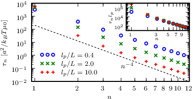
Another way of looking at the chain internal kinetics is through the end-to-end vector MSD, $\Delta_{\text{ee}}(t)\equiv\langle(\mathbf{R}(t)-\mathbf{R}(0))^{2}\rangle$, where $\mathbf{R}(t)=\mathbf{r}(L,t)-\mathbf{r}(0,t)$. For the same parameters used in the top panels of Figs. 3-4, the analogous $\Delta_{\text{ee}}(t)$ results are shown in the bottom panels, together with the corresponding local slopes $\alpha_{\text{ee}}(t)$. The decomposition here is defined with respect to the unit vector $\hat{\mathbf{R}}_{\text{avg}}(t)\equiv(\mathbf{R}(t)+\mathbf{R}(0))/|\mathbf{R}(t)+\mathbf{R}(0)|$, so that $\Delta^{\parallel}_{\text{ee}}(t)=\langle[(\mathbf{R}(t)-\mathbf{R}(0))\cdot\hat{\mathbf{R}}_{\text{avg}}(t)]^{2}\rangle$, $\Delta^{\perp}_{\text{ee}}(t)=(\Delta_{\text{ee}}(t)-\Delta^{\parallel}_{\text{ee}}(t))/2$. The component $\Delta^{\parallel}_{\text{ee}}(t)$ at short times is approximately equal to the MSD of the projected length, $\Delta_{\text{proj}}(t)=\langle(R(t)-R(0))^{2}\rangle$, where $R(t)=|\mathbf{R}(t)|$. This is a well-studied quantity for characterizing semiflexible polymer dynamics [3, 19], and is also plotted in Figs. 3-4. In the stiff limit, the time scale at which $\Delta_{\text{proj}}(t)$ saturates is the upper bound for relaxation of both $\parallel$ and $\perp$ internal contour fluctuations. As can be seen in Figs. 3-4, this saturation time coincides approximately with $\tau_{2}$. Though $\Delta^{\perp}_{\text{ee}}(t)$ continues to grow between $\tau_{2}$ and $\tau_{1}$, the dominant contribution in this range is rotational diffusion of the polymer backbone. The underlying reason is that for $l_{p}/L\to\infty$, the $n=1$ normal mode in the MFT becomes a purely rotational mode [20, 14]. We can see this directly in the plot of $\tau_{n}$ versus $n$ for $L=100a$ and various $l_{p}/L$ in Fig. 5: as we move to stiffer chains, $\tau_{1}$ approaches a constant value, independent of $l_{p}$. Up to a prefactor, this constant agrees with $\tau_{r}\sim L^{3}/\mu_{0}k_{B}T\ln(L/2a)$, the rotational relaxation time of a stiff rod of length $L$ and diameter $2a$. The behavior of $\tau_{n}$ for $n>1$ is quite different: the times scale approximately like $\sim L^{4}/l_{p}n^{4}$ (the inset of Fig. 5 shows data collapse for different $l_{p}$), with corrections due to hydrodynamics. This is exactly the predicted behavior of the relaxation times for transverse fluctuation modes in the weakly bending approach [3].

Thus we can now understand fully the various dynamical regimes seen in both the simulation and MFT results for $\Delta_{\text{end}}(t)$ in the stiff limit. For short times $t\lesssim\tau_{2}$ the motion is dominated by the $\perp$ bending modes of the chain, and we see the characteristic $3/4$ scaling (plus hydrodynamic corrections) in the total MSD curves. Between $\tau_{2}$ and $\tau_{1}$ we have a regime controlled by rotational diffusion: the local slopes increase after $\tau_{2}$, dip sharply through $\tau_{1}$, before rising to 1 at times $t\gg\tau_{1}$, where center-of-mass translational diffusion is dominant. This rotational regime has not been correctly reproduced by any earlier theory based on the weakly-bending assumption. Though the MFT is limited to spatially-averaged properties, it does describe quantitatively the full cross-over between all three regimes, particularly important when making detailed comparisons to experiments.

In summary, we have presented a mean-field approach to semiflexible polymer dynamics that gives a highly accurate description, without fitting parameters, of both experimental FCS measurements on DNA and BD simulations. It incorporates hydrodynamics and works over a wide range of flexibility, even for short, stiff fragments. The latter case is particularly interesting with respect to DNA: there are claims that the elastic energy of the WLC model may no longer be applicable at length scales $\lesssim 100$ nm [21]. If the resolution of FCS experiments could be increased to probe this regime, it would provide a direct and independent test, together with our theory and simulation results, of DNA mechanical properties at these scales, highly relevant to cellular processes.