Magnetic Braiding and Quasi-Separatrix Layers
Abstract
The squashing factor (Titov et al. 2002), a property of the magnetic field line mapping, has been suggested as an indicator for the formation of current sheets, and subsequently magnetic reconnection, in astrophysical plasmas. Here we test this hypothesis for a particular class of braided magnetic fields which serve as a model for solar coronal loops. We explore the relationship between Quasi-Separatrix Layers (QSLs), that is, layer-like structures with high value, electric currents and integrated parallel currents, the latter being a quantity closely related to the reconnection rate. It is found that as the degree of braiding of the magnetic field is increased the maximum values of increase exponentially. At the same time, the distribution of becomes increasingly filamentary, with the width of the high- layers exponentially decreasing. This is accompanied by an increase in the number of layers so that as the field is increasingly braided the volume becomes occupied by a myriad of thin QSLs. QSLs are not found to be good predictors of current features in this class of braided fields. Indeed, despite the presence of multiple QSLs, the current associated with the field remains smooth and large-scale under ideal relaxation; the field dynamically adjusts to a smooth equilibrium. Regions of high are found to be better related to regions of high integrated parallel current than to actual current sheets.
Keywords: magnetohydrodynamics (MHD); magnetic fields; solar corona.
corresponding author: antonia@maths.dundee.ac.uk
1 Introduction
Several different mechanisms have been proposed as explanations for solar coronal heating and indeed it is likely that a number of different heating processes are responsible for the extreme temperature values found. Much of the corona is considered to be close to force-free, that is, in a state satisfying . This consideration led to the proposal of one of the earliest and most debated coronal heating theories, that of topological dissipation (Parker, 1972). Parker theorized that the coronal magnetic field is unable to relax to a smooth force-free equilibrium following arbitrary perturbations of the field via footpoint motions and the consequence is a development of tangential discontinuities in the field. Magnetic reconnection may then occur across the resulting current sheets. Since Parker’s original paper a multitude of arguments for and against the hypothesis have been given but no unanimity presently exists (e.g. van Ballegooijen, 1985; Galsgaard & Nordlund 1996, Craid & Sneyd 2005).
One technique presently employed for predicting current sheet formation in continuous fields is to examine a quantity known as the squashing factor, (Titov et al. 2002; see Appendix A for further details of the function itself). This is a measure for continuous magnetic fields which describes the level of squashing of an infinitesimal flux tube; is large in regions where the footpoint mapping of the field is highly distorted. Regions of very high outline so-called quasi-separatrix layers or QSLs (Priest & Démoulin 1995) and can be considered as an analogue of the separatrix surface in configurations with no null points. QSLs are thought to be sites of preferential current sheet formation (Démoulin et al. 1996; Titov et al. 2002) and a number of numerical experiments have supported this hypothesis (e.g. Longcope & Strauss 1994; Milano et al. 1999; Galsgaard et al. 2003; Aulanier et al. 2005). In addition, observational studies have attempted to examine the relation between QSLs and current sheets (e.g. Schmieder et al. 1997; Fletcher et al. 2001) although this is difficult due to the spatial resolution and quality of the data required for an accurate depiction of the QSLs.
In an earlier paper (Wilmot-Smith et al. 2009) we considered a class of braided magnetic fields. The braids were initially given in closed form (and not in MHD equilibrium), then inserted into a numerical scheme and underwent magnetic relaxation towards a force-free equilibrium. In that paper the current structure of the fields was looked at in some detail. The results are summarized for convenience and put into context in Section 3. Here we return to these models for braided fields in order to examine the relationship between QSLs, currents and a quantity which is important for magnetic reconnection in three dimensions, the electric current integrated along magnetic field lines. As such we begin by describing the braided fields under consideration.
2 Model for a class of braided fields
In Wilmot-Smith et al. 2009, (hereafter Paper I) we introduced a class of braided fields designed to model magnetic fields in solar coronal loops. The fields are given as , , where can be considered as a concatenation of times the ‘elementary’ field . The braided field is modelled on the pigtail braid as illustrated in Figure 1.

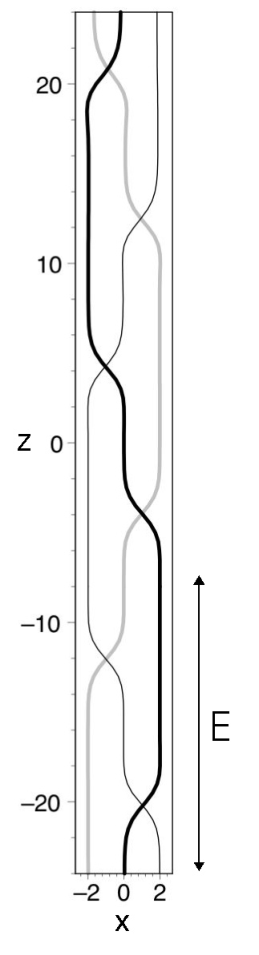
The nature of and the construction mechanism for may be seen from that figure. The field consists of two localized regions of twist in an otherwise uniform field. These two regions are of opposite sign but are of the same underlying form – the superposition onto a uniform vertical field, , of a toroidal flux ring given by
In Cartesian coordinates, placing the centre of this region of toroidal flux at the point we have
| (1) |
where and is taken throughout. The closed form expression for is given by
where and and, similarly, that for by
with appropriate choices for the parameters . For each field we are able to find the equations of the magnetic field lines in closed form and hence an exact expression for for each can be easily calculated.
3 Current structures
In paper I a Lagrangian numerical scheme (Craig & Sneyd, 1986) was used to carry out an ideal relaxation of towards a force-free state with the field on the boundaries of the domain fixed. The maximum Lorentz force within the domain decreased by two orders of magnitude during the relaxation and the resultant field is close to force-free (for a precise definition of what is meant by ‘close’ see Section 3.2 of Paper I). Beyond this point problems with the numerical accuracy of the scheme (Pontin et al., 2009) mean no further relaxation is possible until the numerical difficulties are resolved. In the relaxed state for the current is smooth and of a large-scale (see Figure 3 of Paper I) – two regions of current extend vertically throughout the domain and the maximum magnitude of the current, (), is around half of that of the initial state. No evidence for current sheet formation in the ideal relaxation was found.
It is well known that continuous motions on the boundary of an initially smooth magnetic field cannot lead to truely singular current sheets under an ideal (line–tied) evolution (Van Ballegooijen 1985). However it might seem that the lack of current sheets in our relaxed state contradicts previous results, for example those of Longbottom et al. (1998) and Galsgaard et al. (2003). These investigations found the formation current concentrations under shearing motions on the boundary of an initially current-free configuration. Since we can think of our braid as having been created by a sequence of such shearing motions applied to an initially homogenous field, we might also expect to find similar current concentrations in the relaxed state. A closer comparison, however, shows that the twist, measured by the ratio of the displacement distance () to the length of the domain () in which current concentration are observed is comparatively high in the experiments of Longbottom et al. (1998) and Galsgaard et al (2003). In particular, Longbottom et al. (1998) looked in detail into this question and found significant build-up of current for values above (= ‘shear amplitude’ in their terminology and ). If we were to create our elementary braid (which comes closest to the configuration they considered) by a similar shearing pattern, we would obtain a ratio (; ). This is a value for which no noticeable current concentration has been observed (see Figure 2 of Longbottom et al. 1998) in agreement with our findings. A similar argument applies to the conditions under which Galsgaard et al. (2003) found current concentrations, although their experiment does not allow a direct comparison as they used a resistive code. In their case, values of ( ‘shear distance’ in their terminology, ) below also showed no significant build up of current.
While this shows that our results do not contradict previous findings of current sheet formation, it is perhaps still surprising that a smooth near force-free equilibrium for such a complex configuration exists. In order to understand this one has to bear in mind that our equilibrium is not an exact force-free state but only close to a force-free state (for an exact definition how close see Section 3.2 of paper I). If the residual forces in the relaxed state could be balanced by a pressure, our relaxed state would have a plasma beta of ; although this is well within the quality of ‘force-freeness’ usually assumed for magnetic loops in the solar corona, it is not zero. Moreover, the field has comparatively low maximum force-free field parameter (when measured in a dimensionless way) and it is known that for sufficiently small values of this quantity, force-free equilibria exist for arbitrarily braided fields (Bineau, 1972). Unfortunately the proof given does not give an explicit upper bound but only provides the existence of such a number. These two properties, a low and an only approximately force-free state, appear to allow for a sufficiently large space of smooth solutions to encompass the braids we have investigated.
Whilst in two-dimensions the current itself is the crucial quantity for magnetic reconnection, in three-dimensions the integrated parallel electric field along magnetic field lines plays an important role (Hesse & Schindler, 1988). In resistive MHD, the parallel electric field is related to the parallel current by the relation (assuming a uniform resistivity ). Motivated by this consideration, in Paper I we examined the integrated parallel current, hereafter denoted by , in both the initial and relaxed states for . In both cases a highly filamentary structure containing multiple thin layers was found. During the relaxation the spatial structure of was approximately conserved. More generally, by considering for various , the thickness, , of the layers was found to decrease exponentially with (degree of braiding).
A quantity proposed as an indicator for the formation of current sheets (and hence for the occurrence of magnetic reconnection) in continuous fields is known as the squashing factor, (Titov et al. 2002; Titov et al. 2009). Layers in which is large, so-called quasi-separatrix layers (QSL), can be understood as a generalisation of separatrix surfaces for cases where no null points exist in the domain under consideration. Our previous findings motivate a consideration of the nature of in the class of braided magnetic fields . We relate these findings both to the current structure and the integrated parallel current structure of the fields.
4 Squashing factor and QSLs
A method for obtaining the squashing factor in the braided fields considered is outlined Appendix A. Note that for the squashing factor and the newer definition of the slip-squashing factor (Titov 2007, Titov et al. 2009) give the same result since the magnetic field is normal to both -boundaries.
We begin the discussion by considering the simplest field, . Under ideal relaxation towards a force-free equilibrium, the current, , in remains smooth and large-scale, with the maximum value being in the relaxed state (compared with initially).

The squashing factor for is shown in the left-hand image of Figure 2 as a function of field line positions on the lower boundary. High values of (regions where the field line mapping is strongly distorted) are found in two layer-like regions, and the maximum value of is . Contours of the parallel current integrated along field lines, , are shown in the right-hand image of Figure 2. The characteristic scales of are larger than those of and no relation between the two is evident.


Next consider the field , that based on the pigtail braid and on which most of the analysis of Paper I was based. Recall that a smooth equilibrium with only large-scale current structures was obtained in an ideal relaxation of this field.
The squashing factor on the lower boundary of the domain is shown in the left-hand image of Figure 3. Here the maximum value of is (with calculated at points on the lower boundary) and regions of enhanced occur in a multitude of thin layers in a large portion of the domain. Between these layers drops significantly, even to its minimum possible value of in many locations. A typical half-width at half-maximum (HWHM) of the QSLs is or % of the domain width.
The integrated parallel current structure, , for is shown on the lower boundary of in the right-hand image of Figure 3. A resemblance between and is shown, with both quantities having a similar global structure and containing thin layers of approximately equal width. However, is more filamentary than and has a much greater range of values. In order to make a more precise comparison, the reader is referred to the upper panel of Figure 4 where both quantities are shown for only a subsection of the domain.
Finally consider the field . Both and are shown over a subsection of the domain in the lower panel of Figure 4. The structures of the two quantities are highly filamentary, both containing extremely small scales (HWHM of ). It is seen that and here have a strong resemblance in terms of the global pattern of their thin layer-like structures. However, the locations of the regions of high (low) and high (low) do not exactly coincide.


Considering now alone for the various fields , we seek to determine how the maximum value of and the characteristic width (specifically HWHM), , of the layers of high depend on . It is found that the maximum of for , , in the domain increases exponentially with – as shown in Figure 5(a) – for which a best fit line is
In Paper I a linear increase in the maximum of with was found, as expected since the vertical length of the domain is also increasing linearly by construction of the fields. The typical width, , of the regions of enhanced decreases with . More precisely, there is an exponential decrease in with – as demonstrated in Figure 5(b) – for which a best fit line is
In Paper I a similar exponential decrease in the width () of regions of high was found.
We now address the dependence of the maximum value of , on . Recall that was found to increase exponentially with . Notice that by the construction of we may place an upper bound on the maximum value of from the method of its calculation by composition of matrices. Letting denote the maximum value of for , then the submultiplicative property of the norm tells us that Evaluating, we obtain the upper bound as whilst the true dependence is given by The dependence on the smaller power then comes from the filling factor of the field , i.e. the number of points on the lower boundary of with highest that get mapped under to points with high for the next composition (for etc.)
In the next section we seek to explain these findings and explore theoretically the relationship between and the current structures.
5 Relating QSLs and current structures.
As mentioned above, the squashing factor has been suggested as an indicator for the formation of current sheets. Layers in which is large outline quasi-separatrix layers (QSLs). The link between QSLs and current sheets relies on the following hypothesis (referred to below as the QSL–hypothesis). Where is high there is a sensitive dependence of the end points of magnetic field lines on the starting points (or vice-versa since is symmetric). Hence certain motions of the plasma on one boundary (particularly those crossing the QSLs) would lead to very high velocities at the other boundary, provided the evolution is ideal and the magnetic configuration is unaffected by this perturbation. For sufficiently high this is inconsistent with and so the magnetic configuration has to change. Then a lack of neighbouring smooth equilibria can lead to the formation of current concentrations or even current sheets.
Within the experiments described above we are in a position to test the QSL–hypothesis, given that we can think of the relaxed configuration for as as an ideal deformation of the initial configuration. The initial configuration shows an abundance QSLs but no strong current concentrations. In the subsequent ideal relaxation the QSLs remain but no current sheets (in the sense of a sheet-like structure of ) form. This result appears to contradict the QSL–hypothesis. There are, however, two ways in which the system can escape the necessity of forming current concentrations.
Firstly, the deformation applied could be unfavourable for the formation of current sheets (Titov et al. 2003). For example, Galsgaard et al. (2003) considered a configuration containing two intersection QSLs and applied two types of deformations on the boundary. They found that only one of the types of deformation lead to significant build-up of current.
Given the complexity of our configuration, it seems unlikely that all of the motions which occur during the relaxation are of the type unfavorable for the formation of current sheets unless the nature of the deformation applied () excludes any such favorable deformation. The second possibility is that following the applied deformations the system is able to adjust to a neighbouring smooth equilibrium. This possibility is supported by the arguments given in Section 3 that our final state is a low alpha, near force-free state.
Although current layers are not found in our experiment, it does show layer-like structures of . Such layers have a broader definition in that only the integral of and not itself needs to show small scales. The following example, however, shows that there is no simple relation between either and or between and . We have chosen this example because it is locally similar to the braided fields discussed, in that in both cases and each have a layer-like structure, with multiple layers in which the quantities are enhanced. Consider the force-free magnetic field
for which with , and take , . On the lower boundary, , we have
and
Here the relationship between and currents crucially depends on the choice of parameters. Setting , for example, maxima and minima of , and coincide. Setting instead , then minima in correspond to both maximal and minimal regions of or (see Figure 6). Here we see that the maxima of increase quadratically with the vertical extent () of the domain under consideration, whilst the maxima of increase only linearly and the maxima of are independent of .
Note that this is a specific illustration of a more general case of a force-free field with force-free parameter . Taking then on the lower boundary while and .
The above described situation corresponds well to the braided fields in that both and have a layer-like structure. For we also find that there is no exact correspondence between the layers of high and greatest . However, there is a similarity between and in terms of their global structure, particularly for moderate and large (see Figures 3 and 4). This similarity comes not from an inherent relation between and but rather from the fact that both quantities are functions of the field lines.

To see this, we prescribe a smooth function () of field lines on the lower boundary of each of the braided fields , . We then map this function () along field lines of to the upper boundary, i.e. find . This is demonstrated for a specific example in Figure 7 for , . As is applied repeatedly to any function , then the characteristics of the map will result in a stretching and contracting of in some regions of the domain according to the nature of at those locations, specifically the Lyapunov exponents of the map. After repeated application of any two functions will appear similar; the apparent structure of the two functions will be determined by the mapping .
From this observation we deduce that the structure of both and will depend crucially on the plane in which they are viewed and, by the symmetry of the braid, have the same scale on both the lower and upper boundaries. Accordingly, will, for sufficiently high (about in this case), have a filamentary distribution on the lower boundary that is reflective of the field line mapping rather than the ‘underlying’ nature of the parallel currents. These properties are confirmed by illustrating and for in a cross-section in the middle of the domain (), thereby subtracting as much as possible the effect of the field line mapping. This is shown in Figure 8 where the quantities are seen to attain larger scales than on the domain boundaries and less similarity between and is apparent.


6 Conclusions
In this paper we have examined the link between the squashing factor and current structures in a class of braided magnetic fields. The squashing factor (Titov et al. 2002) is a geometric measure for continuous fields that serves to identify regions where the mapping of magnetic field lines is highly distorted. It is used to identify quasi-separatrix layers (QSLs, Priest & Démoulin 1995) – features of continuous fields which provide an analogue to separatrix surfaces in fields containing null points. Previously, regions of high have been considered to be a reliable indicator for the formation of current sheets under certain deformations on the boundaries.
Here we are interested in both the relationship between and the current , as well as that between and the parallel current integrated along field lines, . The reason for this is that in 3D a key quantity for magnetic reconnection is the parallel electric field integrated along field lines. In resistive MHD with uniform resistivity the parallel electric field and parallel current are related via
We have considered a particular class of braided magnetic fields with no net twist, the fields being labelled (), where an increase in results in a field of increased complexity. In an earlier paper (Wilmot-Smith et al. 2009, Paper I) the field was taken as an initial condition in a magnetic relaxation simulation. The field on the boundaries was held fixed and a magnetofrictional code used to carry out an ideal relaxation toward a force-free equilibrium. In that process the spatial scales associated with the current, , were found to remain large, suggesting a smooth equilibrium corresponding to each can be found.
In Paper I the structure of for was examined. This quantity was shown to display small spatial scales and to have an increasingly filamentary structure with increasing . This structure was preserved in the ideal relaxation process. The consequence was shown to be that for a coronal field with any finite resisitivity, after a certain degree of braiding via photospheric motions the field will undergo a loss of equilibrium due to the high gradients in , regardless of the current structure itself.
Here we have investigated the nature of the squashing factor and associated QSLs for the fields . A method was given (Appendix A) to calculate exactly, a property that becomes important in the analysis where extremely small scales in the quantity are found. It was shown that for the field with the least structure, , is enhanced in two layers of width of the domain width, i.e. there are two quasi-separatrix layers (QSLs) present. As the degree of braiding is increased, develops an increasingly filamentary structure, with many narrow layers of enhanced present. These are true layers in the sense that drops to low values between them. The typical width of the layers decreases exponentially with – for a typical layer width is of the domain width. Additionally, with increasing the maximum value of exponentially increases. The result of the braiding process is shown to be that the domain becomes filled with a multitude of QSLs.
Despite these findings, we find that under ideal relaxation the braided fields do not develop any small-scale structures in the current . This demonstrates an alternative to the view that, in a configuration with QSLs (outlined by regions of high ) plasma motion is highly likely to lead to the formation of current sheets along the QSLs – another possibility is that the magnetic field may adjust to a neighbouring smooth equilibrium. This equilibrium may itself still contain QSLs.
We also considered the relationship between and the integrated parallel current, . In the simplest braid, , the two quantities are unrelated. With increasing braid complexity (), and have some similar characteristics; for moderate and large both quantities are filamentary with layer-like regions in which high values are obtained. However, no simple relationship has been found between the locations of maxima in the two quantities.
Appendix A
Here we give a method for calculating the squashing factor in the braided fields . For this we must obtain the mapping of field lines from the lower boundary of the domain to the upper boundary. We make use of a property of the fields , specifically that is a concatenation of times the ‘basic’ field .
Consider first the field (see Equation 1), that is, a single toroidal flux ring imposed on the background uniform field. The equations of the field line passing through the point are obtained by integrating
where the parameter is related to the distance along field lines by . The components of are given by
| X | |||||
| Y | (2) | ||||
| Z |
where
For the field , the two toroidal flux rings have been placed sufficiently far apart compared with their characteristic length scales that the field in a plane equidistant b between them can be approximated as vertical, . Accordingly, we may replace the error functions in Equations (2) by and obtain an expression for the mapping of field lines from the point in a 2D plane (perpendicular to the field) below the single region of twist in to the point in similar a plane above it:
where and
| (3) |
The mapping of field lines from the lower to upper boundary of the field may then be found by composition of with itself using with the relevant parameters for each of the mappings:
where and . A similar mapping, , of the field lines from the lower to the upper boundary of is obtained by repeated composition of . For example, the field line mapping from the lower to upper boundary of is .
The squashing factor for can be found directly from the Jacobian () of the mapping :
where denotes the entrywise norm. In other words, letting
say, then
For the fields the determinant of the Jacobian mapping is exactly unity () since on both boundaries the field is the constant field . This method determines in the initial states for . Since in the ideal relaxation towards a force-free equilibrium the boundaries are held fixed, the structure of on the boundaries of the domain is preserved throughout the experiments.
Using the same approximation as above, we are able to find a closed form expression for the integrated parallel current along field lines in the initial states for . Taking only a single region of toroidal twist, the field line with initial location in a plane below the region has a total integrated parallel current of
where is defined in Eqn. (3). The total integrated parallel current along field lines for may be found using repeated composition of this expression in a manner similar to that used for . Note that in Paper I was evaluated directly via numerical integration.
Bibliography
Aulanier, G., Pariat, E., Démoulin, P., Current sheet formation in quasi-separatrix layers and hyperbolic flux tubes, A&A, 444, 961-976 (2005).
Bineau, M., On the Existence of Force-Free Magnetic Fields, Comm. Pure Appl. Math., 27, 77 (1972)
Craig, I. J. D. and Sneyd, A. D., The Parker Problem and the Theory of Coronal Heating Solar Physics, 232, 4-621(2005).
Fletcher, L., López Fuentes, M. C., Mandrini, C. H., Schmieder, B., Démoulin, P., Mason, H. E., Young, P. R., Nitta, N., A Relationship Between Transition Region Brightenings, Abundances, and Magnetic Topology Solar Physics, 203 255-287 (2001).
Galsgaard, K. and Nordlund, Å, Heating and activity of the solar corona 1. Boundary shearing of an initially homogeneous magnetic field, JGR, 101, 13445-13460 (1996)
Galsgaard, K., Titov, V.S., Neukirch, T., Magnetic pinching of hyperbolic flux tubes. II. Dynamic numerical model ApJ 595 506-516 (2003).
Longcope, D. W., Strauss, H. R., The form of ideal current layers in line-tied magnetic fields, ApJ, 437 851-859 (1994).
Longbottom, A.W, Rickard, G.J., Craig, I.J.D., and Sneyd, A.D., Magnetic flux braiding:Force-free equilibria and current sheets, ApJ 500 471-482 (1998).
Milano, L. J., Dmitruk, P., Mandrini, C. H., Gomez, D. O., Démoulin, P., Quasi-Separatrix Layers in a Reduced Magnetohydrodynamic Model of a Coronal Loop ApJ, 521 889-897 (1999).
Parker, E. N., Topological Dissipation and the Small-Scale Fields in Turbulent Gases, ApJ, 174 499 (1972.)
Pontin, D.I., Hornig, G., Wilmot-Smith, A.L., Craig, I.J.D., Lagrangian relaxation schemes for calculating force-free magnetic fields, and their limitations, ApJ, 700, 1449 (2009)
Priest, E. R., Démoulin, P., Three-dimensional magnetic reconnection without null points. 1. Basic theory of magnetic flipping, JGR, 100 23443-23464 (1995).
Schmieder, B., Aulanier, G., Demoulin, P., van Driel-Gesztelyi, L., Roudier, T., Nitta, N., Cauzzi, G., Magnetic reconnection driven by emergence of sheared magnetic field, A & A 325 1213-1225 (1997).
Titov, V. S., Generalized Squashing Factors for Covariant Description of Magnetic Connectivity in the Solar Corona, ApJ, 660, 863 (2007).
Titov, V. S. and Galsgaard, K. and Neukirch, T., Magnetic Pinching of Hyperbolic Flux Tubes. I. Basic Estimations, ApJ, 582, 1172 (2003).
Titov, V. S., Hornig, G., Démoulin, P., Theory of magnetic connectivity in the solar corona, JGR (Space Physics) 107, 1164 (2002).
Titov, V. S., Forbes, T. G., Priest, E. R., Mikic, Z., Linker, J. A., Slip-Squashing Factors as a Measure of Three-Dimensional Magnetic Reconnection, ApJ, 693, 1029 (2009).
Van Ballegooijen, A. A., Electric currents in the solar corona and the existence of magnetostatic equilibrium, ApJ, 298, 421-430 (1985)
Wilmot-Smith, A. L., Hornig, G., Pontin, D. I., Magnetic Braiding and Parallel Electric Fields, ApJ, 696, 1139 (2009).