Message Passing Algorithms
for Compressed Sensing
Abstract
Compressed sensing aims to undersample certain high-dimensional signals, yet accurately reconstruct them by exploiting signal characteristics. Accurate reconstruction is possible when the object to be recovered is sufficiently sparse in a known basis. Currently, the best known sparsity-undersampling tradeoff is achieved when reconstructing by convex optimization – which is expensive in important large-scale applications.
Fast iterative thresholding algorithms have been intensively studied as alternatives to convex optimization for large-scale problems. Unfortunately known fast algorithms offer substantially worse sparsity-undersampling tradeoffs than convex optimization.
We introduce a simple costless modification to iterative thresholding making the sparsity-undersampling tradeoff of the new algorithms equivalent to that of the corresponding convex optimization procedures. The new iterative-thresholding algorithms are inspired by belief propagation in graphical models.
Our empirical measurements of the sparsity-undersampling tradeoff for the new algorithms agree with theoretical calculations. We show that a state evolution formalism correctly derives the true sparsity-undersampling tradeoff. There is a surprising agreement between earlier calculations based on random convex polytopes and this new, apparently very different theoretical formalism.
I Introduction and overview
Compressed sensing refers to a growing body of techniques that ‘undersample’ high-dimensional signals and yet recover them accurately [1, 2]. Such techniques make fewer measurements than traditional sampling theory demands: rather than sampling proportional to frequency bandwidth, they make only as many measurements as the underlying ‘information content’ of those signals. However, as compared with traditional sampling theory, which can recover signals by applying simple linear reconstruction formulas, the task of signal recovery from reduced measurements requires nonlinear, and so far, relatively expensive reconstruction schemes. One popular class of reconstruction schemes uses linear programming (LP) methods; there is an elegant theory for such schemes promising large improvements over ordinary sampling rules in recovering sparse signals. However, solving the required LPs is substantially more expensive in applications than the linear reconstruction schemes that are now standard. In certain imaging problems, the signal to be acquired may be an image with pixels and the required LP would involve tens of thousands of constraints and millions of variables. Despite advances in the speed of LP, such problems are still dramatically more expensive to solve than we would like.
This paper develops an iterative algorithm achieving reconstruction performance in one important sense identical to LP-based reconstruction while running dramatically faster. We assume that a vector of measurements is obtained from an unknown -vector according to , where is the measurement matrix . Starting from an initial guess , the first order approximate message passing (AMP) algorithm proceeds iteratively according to:
| (1) | |||||
| (2) |
Here are scalar threshold functions (applied componentwise), is the current estimate of , and is the current residual. denotes transpose of . For a vector , . Finally .
Iterative thresholding algorithms of other types have been popular among researchers for some years, the focus being on schemes of the form
| (3) | |||||
| (4) |
Such schemes can have very low per-iteration cost and low storage requirements; they can attack very large scale applications, - much larger than standard LP solvers can attack. However, [3]-[4] fall short of the sparsity-undersampling tradeoff offered by LP reconstruction [3].
Iterative thresholding schemes based on [3], [4] lack the crucial term in [2] – namely, is not included. We derive this term from the theory of belief propagation in graphical models, and show that it substantially improves the sparsity-undersampling tradeoff.
Extensive numerical and Monte Carlo work reported here shows that AMP, defined by eqns [1], [2] achieves a sparsity-undersampling tradeoff matching the theoretical tradeoff which has been proved for LP-based reconstruction. We consider a parameter space with axes quantifying sparsity and undersampling. In the limit of large dimensions , the parameter space splits in two phases: one where the MP approach is successful in accurately reconstructing and one where it is unsuccessful. References [4, 5, 6] derived regions of success and failure for LP-based recovery. We find these two ostensibly different partitions of the sparsity-undersampling parameter space to be identical. Both reconstruction approaches succeed or fail over the same regions, see Figure 1.
Our finding has extensive empirical evidence and strong theoretical support. We introduce a state evolution formalism and find that it accurately predicts the dynamical behavior of numerous observables of the AMP algorithm. In this formalism, the mean squared error of reconstruction is a state variable; its change from iteration to iteration is modeled by a simple scalar function, the MSE map. When this map has nonzero fixed points, the formalism predicts that AMP will not successfully recover the desired solution. The MSE map depends on the underlying sparsity and undersampling ratios, and can develop nonzero fixed points over a region of sparsity/undersampling space. The region is evaluated analytically and found to coincide very precisely (ie. within numerical precision) with the region over which LP-based methods are proved to fail. Extensive Monte Carlo testing of AMP reconstruction finds the region where AMP fails is, to within statistical precision, the same region.
In short we introduce a fast iterative algorithm which is found to perform as well as corresponding linear programming based methods on random problems. Our findings are supported from simulations and from a theoretical formalism.
Remarkably, the success/failure phases of LP reconstruction were previously found by methods in combinatorial geometry; we give here what amounts to a very simple formula for the phase boundary, derived using a very different and seemingly elegant theoretical principle.
I-A Underdetermined Linear Systems
Let be the signal of interest. We are interested in reconstructing it from the vector of measurements , with , for . For the moment, we assume the entries of the measurement matrix are independent and identically distributed normal .
We consider three canonical models for the signal and three nonlinear reconstruction procedures based on linear programming.
: is nonnegative, with at most entries different from . Reconstruct by solving the LP: minimize subject to , and .
: has as many as nonzero entries. Reconstruct by solving the minimum norm problem: minimize , subject to . This can be cast as an LP.
: , with at most entries in the interior . Reconstruction by solving the LP feasibility problem: find any vector with .
Despite the fact that the systems are underdetermined, under certain conditions on these procedures perfectly recover . This takes place subject to a sparsity-undersampling tradeoff namely an upper bound on the signal complexity relative to and .
I-B Phase Transitions
The sparsity-undersampling tradeoff can most easily be described by taking a large-system limit. In that limit, we fix parameters in and let with and . The sparsity-undersampling behavior we study is controlled by , with the undersampling fraction and a measure of sparsity (with larger corresponding to more complex signals).
The domain has two phases, a ‘success’ phase, where exact reconstruction typically occurs, and a ‘failure’ phase were exact reconstruction typically fails. More formally, for each choice of there is a function whose graph partitions the domain into two regions. In the ‘upper’ region, where , the corresponding LP reconstruction fails to recover , in the following sense: as in the large system limit with and , the probability of exact reconstruction tends to zero exponentially fast. In the ‘lower’ region, where , LP reconstruction succeeds to recover , in the following sense: as in the large system limit with and , the probability of exact reconstruction tends to one exponentially fast. We refer to [4, 5, 7, 6] for proofs and precise definitions of the curves .

The three functions , , are shown in Figure 1; they are the red, blue, and green curves, respectively. The ordering (red blue) says that knowing that a signal is sparse and positive is more valuable than only knowing it is sparse. Both the red and blue curves behave as as ; surprisingly large amounts of undersampling are possible, if sufficient sparsity is present. In contrast, (green curve) for so the bounds are really of no help unless we use a limited amount of undersampling, i.e. by less than a factor of two.
Explicit expressions for are given in [4, 5]; they are quite involved and use methods from combinatorial geometry. By Finding 1 below, they agree to within numerical precision to the following formula:
| (5) |
where , respectively for , . This formula, a principal result of this paper, uses methods unrelated to combinatorial geometry.
I-C Iterative Approaches
Mathematical results for the large-system limit correspond well to application needs. Realistic modern problems in spectroscopy and medical imaging demand reconstructions of objects with tens of thousands or even millions of unknowns. Extensive testing of practical convex optimizers in these problems [8] has shown that the large system asymptotic accurately describes the observed behavior of computed solutions to the above LPs. But the same testing shows that existing convex optimization algorithms run slowly on these large problems, taking minutes or even hours on the largest problems of interest.
Many researchers have abandoned formal convex optimization, turning to fast iterative methods instead [9, 10, 11].
The iteration [1]-[2] is very attractive because it does not require the solution of a system of linear equations, and because it does not require explicit operations on the matrix ; it only requires that one apply the operators and to any given vector. In a number of applications - for example Magnetic Resonance Imaging - the operators which make practical sense are not really Gaussian random matrices, but rather random sections of the Fourier transform and other physically-inspired transforms [2, 12]. Such operators can be applied very rapidly using FFTs, rendering the above iteration extremely fast. Provided the process stops after a limited number of iterations, the computations are very practical.
The thresholding functions in these schemes depend on both iteration and problem setting. In this paper we consider , where is a threshold control parameter, denotes the setting, and is the mean square error of the current current estimate (in practice an empirical estimate of this quantity is used).
For instance, in the case of sparse signed vectors (i.e. problem setting ), we apply soft thresholding , where
where we dropped the argument to lighten notation. Notice that depends on the iteration number only through the mean square error (MSE) .
I-D Heuristics for Iterative Approaches
Why should the iterative approach work, i.e. why should it converge to the correct answer ? The case has been most discussed and we focus on that case for this section. Imagine first of all that is an orthogonal matrix, in particular . Then the iteration [1]-[2] stops in 1 step, correctly finding . Next, imagine that is an invertible matrix; [13], has shown that a related thresholding algorithm with clever scaling of and clever choice of threshold, will correctly find . Of course both of these motivational observations assume , so we are not really undersampling.
We sketch a motivational argument for thresholding in the truly undersampled case which is statistical, which has been popular with engineers [12] and which leads to a proper ‘psychology’ for understanding our results. Consider the operator , and note that . If were orthogonal, we would of course have , and the iteration would, as we have seen immediately succeed in one step. If is a Gaussian random matrix and , then of course is not invertible and is not . Instead of , in the undersampled case behaves as a kind of noisy random vector, i.e. . Now is supposed to be a sparse vector, and, one can see, the noise term is accurately modeled as a vector with i.i.d. Gaussian entries with variance .
In short, the first iteration gives us a ‘noisy’ version of the sparse vector we are seeking to recover. The problem of recovering a sparse vector from noisy measurements has been heavily discussed [14] and it is well understood that soft thresholding can produce a reduction in mean-squared error when sufficient sparsity is present and the threshold is chosen appropriately. Consequently, one anticipates that will be closer to than .
At the second iteration, one has . Naively, the matrix does not correlate with or , and so we might pretend that is again a Gaussian vector whose entries have variance . This ‘noise level’ is smaller than at iteration zero, and so thresholding of this noise can be anticipated to produce an even more accurate result at iteration two; and so on.
There is a valuable digital communications interpretation of this process. The vector is the cross-channel interference or mutual access interference (MAI), i.e. the noiselike disturbance each coordinate of experiences from the presence of all the other ‘weakly interacting’ coordinates. The thresholding iteration suppresses this interference in the sparse case by detecting the many ‘silent’ channels and setting them a priori to zero, producing a putatively better guess at the next iteration. At that iteration, the remaining interference is proportional not to the size of the estimand, but instead to the estimation error, i.e. it is caused by the errors in reconstructing all the weakly interacting coordinates; these errors are only a fraction of the sizes of the estimands and so the error is significantly reduced at the next iteration.
I-E State Evolution
The above ‘sparse denoising’/‘interference suppression’ heuristic, does agree qualitatively with the actual behavior one can observe in sample reconstructions. It is very tempting to take it literally. Assuming it is literally true that the MAI is Gaussian and independent from iteration to iteration, we can can formally track the evolution, from iteration to iteration, of the mean-squared error.

This gives a recursive equation for the formal MSE, i.e. the MSE which would be true if the heuristic were true. This takes the form
| (10) | |||||
| (11) |
Here expectation is with respect to independent random variables and , whose distribution coincides with the empirical distribution of the entries of . We use soft thresholding (I-C) if the signal is sparse and signed, i.e. if . In the case of sparse non-negative vectors, , we will let . Finally, for , we let . Calculations of this sort are familiar from the theory of soft thresholding of sparse signals; see the Supplement for details.
We call the MSE map.
Definition I.1.
Given implicit parameters , with the distribution of the random variable . State Evolution is the recursive map (one-dimensional dynamical system): .
Implicit parameters stay fixed during the evolution. Equivalently, the full state evolves by the rule
Parameter space is partitioned into two regions:
Region (I): for all . Here as : the SE converges to zero.
Region (II): The complement of Region (I). Here, the SE recursion does not evolve to .
The partitioning of parameter space induces a notion of sparsity threshold, the minimal sparsity guarantee needed to obtain convergence of the formal MSE:
| (12) |
The subscript SE stands for State Evolution. Of course, depends on the case ; it also seems to depend also on the signal distribution ; however, an essential simplification is provided by
Proposition I.2.
For the three canonical problems , any , and any random variable with the prescribed sparsity and bounded second moment, is independent of .
Independence from allows us to write for the sparsity thresholds. The proof of this statement is sketched below, along with the derivation of a more explicit expression. Adopt the notation
| (13) |
High precision numerical evaluations of such expression uncovers the following very suggestive
Finding 1.
For the three canonical problems , and for any
| (14) |
In short, the formal MSE evolves to zero exactly over the same region of phase space as does the phase diagram for the corresponding convex optimization!
I-F Failure of standard iterative algorithms
If we trusted that formal MSE truly describes the evolution of the iterative thresholding algorithm, Finding 1 would imply that iterative thresholding allows to undersample just as aggressively in solving underdetermined linear systems as the corresponding LP.
Finding 1 gives new reason to hope for a possibility that has already inspired many researchers over the last five years: the possibility of finding a very fast algorithm that replicates the behavior of convex optimization in settings .
Unhappily the formal MSE calculation does not describe the behavior of iterative thresholding:
1. State Evolution does not predict the observed properties of iterative thresholding algorithms.
2. Iterative thresholding algorithms, even when optimally tuned, do not achieve the optimal phase diagram.
In [3], two of the authors carried out an extensive empirical study of iterative thresholding algorithms. Even optimizing over the free parameter and the nonlinearity the phase transition was observed at significantly smaller values of than those observed for LP-based algorithms.
Numerical simulations also show very clearly that the MSE map does not describe the evolution of the actual MSE under iterative thresholding. The mathematical reason for this failure is quite simple. After the first iteration, the entries of become strongly dependent, and State Evolution does not predict the moments of .
I-G Message Passing Algorithm
The main surprise of this paper is that this failure is not the end of the story. We now consider a modification of iterative thresholding inspired by message passing algorithms for inference in graphical models [16], and graph-based error correcting codes [17, 18]. These are iterative algorithms, whose basic variables (‘messages’) are associated to directed edges in a graph that encodes the structure of the statistical model. The relevant graph here is a complete bipartite graph over nodes on one side (‘variable nodes’), and on the others (‘measurement nodes’). Messages are updated according to the rules
| (15) |
| (16) |
for each . We will refer to this algorithm11 1 For earlier applications of MP to compressed sensing see [19, 20, 21]. Relations between MP and LP were explored in a number of papers, see for instance [22, 23], albeit from a different perspective. as to MP.
MP has one important drawback with respect to iterative thresholding. Instead of updating estimates, at each iterations we need to update messages, thus increasing significantly the algorithm complexity. On the other hand, it is easy to see that the right-hand side of eqn [15] depends weakly on the index (only one out of terms is excluded) and that the right-hand side of eqn [15] depends weakly on . Neglecting altogether this dependence leads to the iterative thresholding equations [3], [4]. A more careful analysis of this dependence leads to corrections of order one in the high-dimensional limit. Such corrections are however fully captured by the last term on the right hand side of eqn [2], thus leading to the AMP algorithm. Statistical physicists would call this the ‘Onsager reaction term’; see [24].

I-H State Evolution is Correct for MP
Although AMP seems very similar to simple iterative thresholding [3]-[4], SE accurately describes its properties, but not those of the standard iteration. As a consequence of Finding 1, properly tuned versions of MP-based algorithms are asymptotically as powerful as LP reconstruction.
We have conducted extensive simulation experiments with AMP, and more limited experiments with MP, which is computationally more intensive (for details see the complementary material). These experiments show that the performance of the algorithms can be accurately modeled using the MSE map. Let’s be more specific.
According to SE, performance of the AMP algorithm is predicted by tracking the evolution of the formal MSE via the recursion [10]. Although this formalism is quite simple, it is accurate in the high dimensional limit. Corresponding to the formal quantities calculated by SE are the actual quantities, so of course to the formal MSE corresponds the true MSE . Other quantities can be computed in terms of the state as well: for instance the true false alarm rate is predicted via the formal false alarm rate . Analogously, the true missed-detection rate is predicted by the formal missed-detection rate , and so on.
Our experiments establish agreement of actual and formal quantities.
Finding 2.
For the AMP algorithm, and large dimensions , we observe
I. SE correctly predicts the evolution of numerous statistical properties of with the iteration number . The MSE, the number of nonzeros in , the number of false alarms, the number of missed detections, and several other measures all evolve in way that matches the state evolution formalism to within experimental accuracy.
II. SE correctly predicts the success/failure to converge to the correct result. In particular, SE predicts no convergence when , and convergence if . This is indeed observed empirically.
Analogous observations were made for MP.
I-I Optimizing the MP Phase Transition
An inappropriately tuned version of MP/AMP will not perform well compared to other algorithms, for example LP-based reconstructions. However, SE provides a natural strategy to tune MP and AMP (i.e. to choose the free parameter ): simply use the value achieving the maximum in eqn [13]. We denote this value by , , and refer to the resulting algorithms as to optimally tuned MP/AMP (or sometimes MP/AMP for short). They achieve the State Evolution phase transition:
An explicit characterization of , can be found in the next section.
We summarize below the properties of optimally tuned AMP/MP within the SE formalism.
Theorem I.3.
For , , and any associated random variable , the formal MSE of optimally-tuned AMP/MP evolves to zero under SE. Viceversa, if , the formal MSE does not evolve to zero. Further, for , there exists with the following property. If denotes the formal MSE after SE steps, then, for all
| (17) |
II Details About the MSE Mapping
In this section, we sketch the proof of Proposition I.2: the iterative threshold does not depend on the details of the signal distribution. Further, we show how to derive the explicit expression for , , given in the introduction.
II-A Local Stability Bound
The state evolution threshold is the supremum of all ’s such that the MSE map lies below the line for all . Since , for this to happen it must be true that the derivative of the MSE map at smaller than or equal to . We are therefore led to define the following ‘local stability’ threshold:
| (18) |
The above argument implies that .
Considering for instance , we obtain the following expression for the first derivative of
where is the standard Gaussian density at and is the Gaussian distribution.
Evaluating this expression as , we get the local stability threshold for :
where is the same as in [5]. Notice that depends on the distribution of only through its sparsity (i.e. it is independent of ).
II-B Tightness of the Bound and Optimal Tuning
We argued that is necessary for the MSE map to converge to . This condition turns out to be sufficient because the function is concave on . This indeed yields
| (19) |
which implies exponential convergence to the correct solution [17]. In particular we have
| (20) |
whence is independent of as claimed.
To prove is concave, one proceeds by computing its second derivative. For instance, in the case , one needs to differentiate the expression given above for the first derivative. We omit details but point out two useful remark: The contribution due to vanishes; Since a convex combination of concave functions is also concave, it is sufficient to consider the case in which deterministically.
As a byproduct of this argument we obtain explicit expressions for the optimal tuning parameter, by maximizing the local stability threshold
Before applying this formula in practice, please read the important notice in Supplemental Information.
III Discussion
III-A Relation with Minimax Risk
Let denote the class of probability distributions supported on with , and let denote the soft-threshold function [I-C] with threshold value . The minimax risk [14] is defined as
| (21) |
with the optimal . The optimal SE phase transition and optimal SE threshold obey
| (22) |
An analogous relation holds between the positive case , and the minimax threshold risk where is constrained to be a distribution on . Exploiting [22], Supporting Information proves that
III-B Other Message Passing Algorithms
The nonlinearity in AMP eqns [1], [2] might be chosen differently. For sufficiently regular such choices, the SE formalism might predict evolution of the MSE. One might hope to use SE to design ‘better’ threshold nonlinearities.
The threshold functions used here are such that the MSE map is monotone and concave. As a consequence, the phase transition line for optimally tuned AMP is independent of the empirical distribution of the vector . State Evolution may be inaccurate without such properties.
Where SE is accurate, it offers limited room for improvement over the results here. If denotes a (hypothetical) phase transition derived by SE with any nonlinearity whatsoever, Supporting Information exploits [22] to prove
In the limit of high undersampling, the nonlinearities studied here offer essentially unimprovable SE phase transitions. Our reconstruction experiments also suggest that other nonlinearities yield little improvement over thresholds used here.
III-C Universality
The SE-derived phase transitions are not sensitive to the detailed distribution of coefficient amplitudes. Empirical results in Supporting Information find similar insensitivity of observed phase transitions for MP.
Gaussianity of the measurement matrix can be relaxed; Supporting Information finds that other random matrix ensembles exhibit comparable phase transitions.
In applications, one often uses very large matrices which are never explicitly represented, but only applied as operators; examples include randomly undersampled partial Fourier transforms. Supporting Information finds that observed phase transitions for MP in the partial Fourier case are comparable to those for random .
Acknowledgements
A. Montanari was partially supported by the NSF CAREER award CCF-0743978 and the NSF grant DMS-0806211, and thanks Microsoft Research New England for hospitality during completion of this work. A. Maleki was partially supported by NSF DMS-050530.
References
- [1] D. L. Donoho, “Compressed Sensing,” IEEE Transactions on Information Theory, Vol. 52, pp. 489-509, April 2006.
- [2] E. Candès, J. Romberg, T. Tao, “Robust uncertainty principles: Exact signal reconstruction from highly incomplete frequency information,” IEEE Transactions on Information Theory,Vol. 52, No. 2, pp. 489-509, February 2006.
- [3] A. Maleki, D. L. Donoho, “Optimally Tuned Iterative Thresholding Algorithms,” submitted to IEEE journal on selected areas in signal processing, 2009.
- [4] D. L. Donoho, “High-Dimensional centrally symmetric polytopes with neighborliness proportional to dimension,” Discrete and Computational Geometry, Vol 35,No. 4, pp. 617-652, 2006.
- [5] D. L. Donoho, J. Tanner, “Neighborliness of randomly-projected simplices in high dimensions,” Proceedings of the National Academy of Sciences, Vol. 102, No. 27, p. 9452-9457, 2005.
- [6] D. L. Donoho, J. Tanner, “Counting faces of randomly projected hypercubes and orthants, with applications,” ArXiv.
- [7] D. L. Donoho, J. Tanner, “Counting faces of randomly projected polytopes when the projection radically lowers dimension,” J. Amer. Math. Soc., Vol. 22, pp. 1-53, 2009.
- [8] D. L. Donoho, J.Tanner, “Observed universality of phase transitions in high dimensional geometry, with implication for modern data analysis and signal processing,” Phil. Trans. A, 2009.
- [9] K. K. Herrity, A. C. Gilbert, and J. A. Tropp, “Sparse approximation via iterative thresholding,” Proc. ICASSP, Vol. 3, pp. 624-627, Toulouse, May 2006.
- [10] J. A. Tropp, A. C. Gilbert,“ Signal recovery from random measurements via orthogonal matching pursuit,” IEEE Transactions Information Theory, 53(12),pp. 4655-4666, 2007.
- [11] P. Indyk, M. Ruzic, “Near optimal sparse recovery in the norm,” In th Annual Symposium on Foundations of Computer Science, pp. 199-207, Philadelphia, PA, October 2008.
- [12] M. Lustig, D. L. Donoho, J. M. Santos, J. M. Pauly, “Compressed sensing MRI,” IEEE Signal Processing Magazine, 2008.
- [13] I. Daubechies, M. Defrise and C. De Mol, “An iterative thresholding algorithm for linear inverse problems with a sparsity constraint,” Communications on Pure and Applied Mathematics, Vol. 75, pp. 1412-1457, 2004.
- [14] D. L. Donoho, I. M. Johnstone, “Minimax risk over balls,” Prob. Th. and Rel. Fields, Vol. 99, pp. 277-303, 1994.
- [15] D. L. Donoho, I. M. Johnstone, “Ideal spatial adaptation via wavelet shrinkage,” Biometrica, Vol. 81, pp. 425-455, 1994.
- [16] J. Pearl, Probabilistic reasoning in intelligent systems: networks of plausible inference, Morgan Kaufmann, San Francisco, 1988.
- [17] R. G. Gallager, Low-Density Parity-Check Codes, MIT Press, Cambridge, Massachusetts, 1963, Available online at: http://web./gallager/www/pages/ldpc.pdf.
- [18] T. J. Richardson, R. Urbanke, Modern coding theory, Cambridge University Press, Cambridge,2008, Available online at: http://lthcwww.epfl.ch/mct/index.php.
- [19] Y. Lu, A. Montanari, B. Prabhakar, S. Dharmapurikar and A. Kabbani, “Counter Braids: a novel counter architecture for per-flow measurement,” SIGMETRICS, Annapolis, June 2008.
- [20] S. Sarvotham, D. Baron and R. Baraniuk, “Compressed sensing reconstruction via belief propagation,” Preprint, 2006.
- [21] F. Zhang, H. Pfister,“On the iterative decoding of high-rate LDPC codes with applications in compressed sensing,” arXiv:0903.2232v2, 2009.
- [22] M. J. Wainwright, T. S. Jaakkola and A. S. Willsky,“MAP estimation via agreement on trees: message-passing and linear programming,” IEEE Transactions on Information Theory, Vol. 51, No. 11, pp. 3697-3717.
- [23] M. Bayati, D. Shah and M. Sharma, “ Max-Product for maximum weight matching: convergence, correctness, and LP duality,” IEEE Transactions on Information Theory, Vol. 54, No. 3, pp. 1241-1251, 2008.
- [24] D. J. Thouless, P. W. Anderson and R. G. Palmer, “ Solution of solvable model of a spin glass,” Phil. Mag., Vol. 35, pp. 593-601, 1977.
- [25] D. L. Donoho and I.M. Johnstone and J.C. Hoch and A.S. Stern, “Maximum Entropy and the Nearly Black Object,” Journal of the Royal Statistical Society, Series B (Methodological), Vol. 54, pp. 41-81, 1992.
- [26] D. L. Donoho, J. Tanner, “Phase transition as sparse sampling theorems,” IEEE Transactions on Information Theory,submitted for publication.
- [27] P. J. Bickel, “Minimax estimation of the mean of a normal distribution subject to doing well at a point,” in Recent Advances in Statistics: Papers in Honor of Herman Chernoff on His Sixtieth Birthday, Academic Press, 511-528, 1983.
- [28] B. Efron and T. Hastie and I. Johnstone and R. Tibshirani, “Least angle regression,” Annals of Statistics, Vol.32, pp. 407-492, 2004.
-D Important Notice
Readers familiar with the literature of thresholding of sparse signals will want to know that an implicit rescaling is needed to match equations from that literature with equations here. Specifically, in the traditional literature, one is used to seeing expressions in cases where is the standard deviation of an underlying normal distribution. This means the threshold is specified in standard deviations, so many people will immediately understand values like of etc in terms of their false alarm rates. In the main text, the expression appears numerous times, but note that is not the standard deviation of the relevant normal distribution; instead, the standard deviation of that normal is . It follows that in the main text is calibrated differently from the way would be calibrated in other sources, differing by a -dependent scale factor. If we let denote the quantity appropriately rescaled so that it is in units of standard deviations of the underlying normal distribution, then the needed conversion to sd units is
| (23) |
-E A summary of notation
The main paper will be referred as DMM throughout this note. All the notations are consistent with the notations used in DMM. We will use repeatedly the notation .
-F State Evolution Formulas
In the main text we mentioned is independent of . We also mentioned a few formulas for . The goal of this section is to explain the calculations involved in deriving these results. First, recall the expression for the MSE map
| (24) |
We denote by and the partial derivatives of with respect to its first and second arguments. Using Stein’s lemma and the fact that almost everywhere, we get
| (25) |
where we dropped the dependence of on the constraint to simplify the formula.
-F1 Case
In this case we have almost surely and the threshold function is
As a consequence (almost everywhere). This yields
As , we have and if . Therefore,
The local stability threshold is obtained by setting .
In order to prove the concavity of first notice that a convex combination of concave functions is concave and so it is sufficient to show the concavity in the case deterministically. Next notice that, in the case , is independent of . A a consequence, it is sufficient to prove where
Using and , we get
| (28) |
for .
-F2 Case
Here is supported on with . Recall the definition of soft threshold
As a consequence and . This yields
By letting we get
which yields the local stability threshold by .
Finally the proof of the concavity of is completely analogous to the case .
-F3 Case
Finally consider the case of supported on with . In this case we proposed the following nonlinearity,
Notice that the nonlinearity does not depend on any threshold parameter. Since ,
As we get
whence the local stability condition yields .
Concavity of immediately follows from the fact that is non-increasing in for and is non-decreasing for . Using the combinatorial geometry result of [6] we get
Theorem .1.
For any ,
| (35) |
-G Relation to Minimax Thresholding
-G1 Minimax Thresholding Policy
We denote by the collection of all CDF’s supported in and with , and by the collection of all CDF’s supported in and with . For , define the minimax threshold MSE
| (36) |
where denote expectation with respect to the random variable with distribution , and for and for . Minimax Thresholding was discussed for the case in [25] and for in [14, 15].
This machinery gives us a way to look at the results derived above in very commonsense terms. Suppose we know and but not the distribution of . Let’s consider what threshold one might use, and ask at each given iteration of SE, the threshold which gives us the best possible control of the resulting formal MSE. That best possible threshold is by definition the minimax threshold at nonzero fraction , appropriately scaled by the effective noise level ,
where depending on the case at hand. Note that this threshold does not depend on . It depends on iteration only through the effective noise level at that iteration. The guarantee we then get for the formal MSE is the minimax threshold risk, appropriately scaled by the square of the effective noise level:
| (37) |
for . This guarantee gives us a reduction in MSE over the previous iteration if and only if the right-hand side in Eq. (37) is smaller than , i.e. if and only if
In short, we can use state evolution with the minimax threshold, appropriately scaled by effective noise level, and we get a guaranteed fractional reduction in MSE at each iteration, with fractional improvement
| (38) |
hence the formal SE evolution is bounded by:
| (39) |
Results analogous to those of the main text hold for this minimax thresholding policy. That is, we can define a minimax thresholding phase transition such that below that transition, state evolution with minimax thresholding converges:
-G2 Relating Optimal Thresholding to Minimax Thresholding
An important difference between the optimal threshold defined in the main text and the minimax threshold is that depends only on the assumed – no specific need be chosen while minimax thresholding as defined above requires that one specify both and . However, since the methodology is seemingly pointless above the minimax phase transition, one might think to specify . This new threshold then requires no specification of . As it turns out, the SE threshold coincides with this new threshold.
Theorem .3.
For and
| (40) |
Let denote the minimax threshold defined in the main text, and let denote denote the same quantity expressed in sd units (23). Then
Proof.
It is convenient to introduce the following explicit notation for the MSE map:
| (41) |
where is independent of , and . As above, we drop the dependency of the threshold function on Since for any positive , we have the scale invariance
| (42) |
where is the operator that takes the CDF of an random variable and returns the CDF of the random variable .
Define
| (43) |
where . It follows from the definition of SE threshold that if and only if . We first notice that by concavity of , we have
| (44) | |||||
| (45) | |||||
| (46) |
where the second identity follows from the invariance property and the third from the observation that for any . Comparing with the definition (36), we finally obtain
| (47) |
Therefore if and only , which implies the thesis. ∎
-H Convergence Rate of State Evolution
The optimal thresholding policy described in the main text is the same as using the minimax thresholding policy but instead assuming the most pessimistic possible choice of – the largest that can possibly make sense. In contrast minimax thresholding is -adaptive, and can use a smaller threshold where it would be valuable. Below the SE phase transition, both methods will converge, so what’s different?
Note that and are dimensionally different; is in standard deviation units. Converting into sd units by (23), we have . Even after this calibration, we find that methods will generally use different thresholds, i.e. if ,
In consequence, the methods may have different rates of convergence. Define the worst-case threshold MSE
and set
This is the MSE guarantee achieved by using when in fact is the case. Now by definition of minimax threshold MSE,
| (48) |
the inequality is generally strict. The convergence rate of optimal AMP under SE was described implicitly in the main text. We can give more precise information using this notation. Define
Then we have for the formal MSE of AMP
In the main text, the same relation was written in terms of , with ; here we see that we may take . Explicit evaluation of this requires evaluation of the worst-case thersholding risk . Now by (48) we have
generally with strict inequality; so by using the -adaptive threshold one gets better speed guarantees.
-I Rigorous Asymptotic Agreement of SE and CG
In this section we prove
Theorem .4.
For
| (49) |
In words, is the phase transition computed by combinatorial geometry (polytope theory) and obtained by state evolution: they are rigorously equivalent in the highly undersampled limit (i.e. limit). In the main text, we only can make the observation that they agree numerically.
-I1 Properties of the minimax threshold
We summarize here several known properties of the minimax threshold (36), which provide useful information about the behavior of SE.
The extremal achieving the supremum in Eq. (36) is known. In the case , it is a two-point mixture
| (50) |
In the signed case , it is a three-point symmetric mixture
| (51) |
Precise asymptotic expressions for are available. In particular, for ,
| (52) |
We also know that
| (53) |
-I2 Proof of Theorem .4
Combining Theorem .3 and Eq. (53), we get
| (54) |
(correction terms that can be explicitly given). Now we know rigorously from [26] that the LP-based phase transitions satisfy a similar relationship:
Theorem .5 (Donoho and Tanner [26]).
For
| (55) |
-J Rigorous Asymptotic Optimality of Soft Thresholding
The discussion in the main text, alluded to the possibility of improving on soft thresholding. Here we give a more formal discussion. We work in the situations . Let denote some arbitrary nonlinearity with tuning parameter . (For a concrete example, think of hard thresholding). We can define the minimax MSE for this nonlinearity in the natural way
| (56) |
there is a corresponding minimax threshold . We can deploy the minimax threshold in AMP by setting and rescaling the threshold by the effective noise level :
| actual threshold at iteration | ||||
Under state evolution, this is guaranteed to reduce the MSE provided
In that case we get full evolution to zero. It makes sense to define the minimax phase transition:
Whatever be , for with , SE evolves the formal MSE of to zero.
It is tempting to hope that some very special nonlinearity can do substantially better than soft thresholding. At least for the minimax phase transition, this is not so:
Theorem .6.
Let be a minimax phase transition computed under the State Evolution formalism for the cases with some scalar nonlinearity . Let be the phase transition calculated in the main text for soft thresholding with corresponding optimal . Then for
In words, no other nonlinearity can outperform soft thresholding in the limit of extreme undersampling – in the sense of minimax phase transitions. This is best understood using a notion from the main text. We there said that the parameter space can be partitioned into two regions. Region (I) where there zero is the unique fixed point of the MSE map, and is a stable fixed point; and its complement, Region (II). Theorem .6 says that the range of guaranteeing membership in Region (I) cannot be dramatically expanded by using a different nonlinearity.
-J1 Some results on Minimax Risk
The proof depends on some know results about minimax MSE, where we are allowed to choose not just the threshold, but also the nonlinearity. For , define the minimax MSE
| (57) |
Here the minimization is over all measurable functions . Minimax MSE was discussed for the case in [25] and for in [27, 14, 15]. It is known that
| (58) |
-K Proof of Theorem .6
-L Data Generation
For a given algorithm with a fully specified parameter vector, we conduct one phase transition measurement experiment as follows. We fix a problem suite, i.e. a matrix ensemble and a coefficient distribution for generating problem instances . We also fix a grid of values in , typically values equispaced between and . Subordinate to this grid, we consider a series of values. Two cases arise frequently:
- •
Focused Search design. 20 values between and , where is the theoretically expected phase transition deriving from combinatorial geometry (according to case ).
- •
General Search design. 40 values equispaced between 0 and 1.
We then have a (possibly non-cartesian) grid of values in parameter space . At each combination, we will take problem instances; in our case . We also fix a measure of success; see below.
Once we specify the problem size , the experiment is now fully specified; we set and , and generate problem instances, and obtain algorithm outputs , and success indicators , .
A problem instance consists of matrix from the given matrix ensemble and a -sparse vector from the given coefficient ensemble. Then . The algorithm is called with problem instance and it produces a result . We declare success if
where is a given parameter; in our case ; the variable indicates success on the -th Monte Carlo realization. To summarize all Monte Carlo repetitions, we set .
The result of such an experiment is a dataset with tuples ; each tuple giving the results at one combination . The meta-information describing the experiment is the specification of the algorithm with all its parameters, the problem suite, and the success measure with its tolerance.
-M Estimating Phase Transitions
From such a dataset we find the location of the phase transition as follows. Corresponding to each fixed value of in our grid, we have a collection of tuples with and varying . Pretending that our random number generator makes truly independent random numbers, the result at one experiment is binomial , where the success probability . Extensive prior experiments show that this probability varies from when is well below to when is well above . In short, the success probability
We define the finite- phase transition as the value of at which success probability is 50%:
This notion is well-known in biometrics where the 50% point of the dose-response is called the LD50. (Actually we have the implicit dependence ; the tolerance in the success definition has a (usually slight) effect, as well as the problem size )
To estimate the phase transition from data, we model dependence of success probability on using generalized linear models (GLMs). We take a -constant slice of the dataset obtaining triples , and model where the success probabilities obeys a generalized linear model with logistic link
where ; in biometric language, we are modeling that the dose-response probability, where is the ‘complexity-dose’, follows a logistic curve.
In terms of the fitted parameters ,, we have the estimated phase transition
and the estimated transition width is
Note that, actually,
We may be able to see the phase transition and its width varying with and with the success tolerance.
Because we make only measurements in our Monte Carlo experiments, these results are subject to sampling fluctuations. Confidence statements can be made for using standard statistical software.
-N Tuning of Algorithms
The procedure so far gives us, for each fully-specified combination of algorithm parameters and each problem suite , a dataset . When an algorithm has such parameters, we can define, for each fixed , the value of the parameters which gives the highest transition:
with associated optimal parameters . When the results of the algorithm depend strongly on problem suite as well, we can also tune to optimize worst-case performance across suites, getting the minimax transition
and corresponding minimax parameters . This procedure was followed in [3] for a wide range of popular algorithms. Figure 3 of the main text presents the observed minimax transitions.
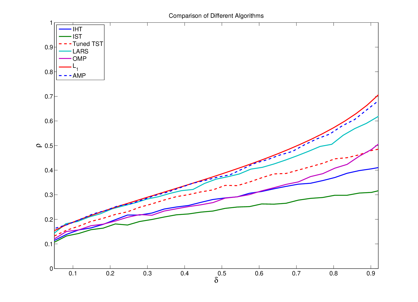
-O Results: Empirical Phase Transition
Figure 4 (which is a complete version of Figure 3 in the main text) compares observed phase transitions of several algorithms including AMP. We considered what was called in [3] the standard suite, wit these choices
- •
Matrix ensemble: Uniform spherical ensemble(USE); each column of is drawn uniformly at random from the unit sphere in .
- •
Coefficient ensemble: The vector has nonzeros in random locations, with constant amplitude of nonzeros. If , ; if , (with equiprobable positive and negative entries).
For each algorithm we generated an appropriate grid of and created independent problem instances at each gridpoint, i.e. independent realizations of vector and measurement matrix .
For AMP we used a focused search design, focused around . To reconstruct , we run AMP iterations and report the mean square error at the final iteration. For other algorithms, we used the general search design as described above. For more details about observed phase transitions we refer the reader to [3].
The calculation of the phase transition curve of AMP takes around hours on a single Pentium processor.
-P Example of the Interference Heuristic
In the main text, our motivation of the SE formalism used the assumption that the mutual access interference term MAI is marginally nearly Gaussian – i.e. the distribution function of the entries in the MAI vector is approximately Gaussian.
As we mentioned, this heuristic motivates the definition of the MSE map. It is easy to prove that the heuristic is valid at the first iteration; but for the validity of SE, it must continue to be true at every iteration until the algorithm stops. Figure 5 presents a typical example. In this example we have considered USE matrix ensemble and Rademacher Coefficient ensemble. Also is set to a small size problem and . The algorithm is tracked across 90 iterations. Each panel exhibits a linear trend, indicating approximate Gaussianity. The slope is decreasing with iteration count. The slope is the square root of the MSE, and its decrease indicates that the MSE is evolving towards zero. More interestingly, figure 6 shows the QQplot of the MAI noise for the partial Fourier matrix ensemble. Coefficients here are again from Rademacher ensemble and .


-Q Testing Predictions of State Evolution


The last section gave an illustration tracking the actual evolution of the AMP algorithm, it showed that the State Evolution heuristic is qualitatively correct.
We now consider predictions made by SE and their quantitative match with empirical observations. We consider predictions of four observables:
- •
MSE on zeros and MSE on non-zeros:
MSEZ MSENZ (59) - •
Missed detection rate and False alarm rate:
MDR FAR (60)
We illustrate the calculation of MDR. Other quantities are computed similarly. Let , and suppose that entries in are either , , or , with . Then, with ,
| (61) | |||||
with , .
In short, the calculation merely requires classical properties of the normal distribution. The three other quantities simply require other similar properties of the normal. As discussed in the main text, SE evolution makes an iteration-by-iteration prediction of ; in order to calculate predictions of MDR, FAR, MSENZ and MSEZ, the parameters and are also needed.
We compared the state evolution predictions with the actual values by a Monte Carlo experiment. We chose these triples : , , . We again used the standard problem suite (USE matrix and unit amplitude nonzero). At each combination of , we generated random problem instances from the standard problem suite, and ran the AMP algorithm for a fixed number of iterations. We computed the observables at each iteration. For example, the empirical missed detection rate is estimated by
We averaged the observable trajectories across the Monte Carlo realizations, producing empirical averages.
The results for the three cases are presented in Figures 7, 8, 9. Shown on the display are curves indicating both the theoretical prediction and the empirical averages. In the case of the upper row and the lower left panel, the two curves are so close that one cannot easily tell that two curves are, in fact, being displayed.
-R Coefficient Universality

SE displays invariance of the evolution results with respect to the coefficient distribution of the nonzeros. What happens in practice?
We studied invariance of AMP results as we varied the distributions of the nonzeros in . We consider the problem and used the following distributions for the non-zero entries of :
- •
Uniform in ;
- •
Radamacher (uniform in );
- •
Gaussian;
- •
Cauchy.
In this study, , and we considered , . For each value of we considered equispaced values of in the interval , running each time AMP iterations. Data are presented, respectively, in Figures 10.
Each plot displays the fraction of success as a function of and a fitted success probability i.e. in terms of success probabilities, the curves display . In each case 4 curves and 4 sets of data points are displayed, corresponding to the 4 ensembles. The four datasets are visually quite similar, and it is apparent that indeed a considerable degree of invariance is present.
-S Matrix Universality
The Discussion section in the main text referred to evidence that our results are not limited to the Gaussian distribution.
We conducted a study of AMP where everything was the same as in Figure 1 above, however, the matrix ensemble could change. We considered three such ensembles: USE (columns iid uniformly distributed on the unit sphere), Rademacher (random entries iid equiprobable), and Partial Fourier, (randomly select rows from fourier matrix.) We only considered the case . Results are shown in Fig. 11, and compared to the theoretical phase transition for .

-T Timing Results
In actual applications, AMP runs rapidly.
We first describe a study comparing AMP to the LARS algorithm [28]. LARS is appropriate for comparison because, among the iterative algorithms previously proposed, its phase transition is closest to the transition. So it comes closest to duplicating the AMP sparsity-undersampling tradeoff.
Each algorithm proceeds iteratively and needs a stopping rule. In both cases, we stopped calculations when the relative fidelity measure exceeded , ie when .
In our study, we used the partial Fourier matrix ensemble with unit amplitude for nonzero entries in the signal . We considered a range of problem sizes and in each case averaged timing results over problem instances. Table I presents timing results.
In all situations studied, AMP is substantially faster than LARS. There are a few very sparse situations – i.e. where is in the tens or few hundreds – where LARS performs relatively well, losing the race by less than a factor 3. However, as the complexity of the objects increases, so that is several hundred or even one thousand, LARS is beaten by factors of 10 or even more.
(For very large , AMP has a decisive advantage. When the matrix is dense, LARS requires at least operations, while AMP requires at most operations. Here is a bound on the number of iterations, and is the relative improvement in MSE in iterations. Hence in terms of flops we have
This logarithmic dependence of the denominator is very weak, and very roughly this ratio scales directly with .)
| AMP | LARS | |||
|---|---|---|---|---|
| 4096 | 820 | 120 | 0.19 | 0.7 |
| 8192 | 1640 | 240 | 0.34 | 3.45 |
| 16384 | 3280 | 480 | 0.72 | 19.45 |
| 32768 | 1640 | 160 | 2.41 | 7.28 |
| 16384 | 820 | 80 | 1.32 | 1.51 |
| 8192 | 820 | 110 | 0.61 | 1.91 |
| 16384 | 1640 | 220 | 1.1 | 5.5 |
| 32768 | 3280 | 440 | 2.31 | 23.5 |
| 4096 | 1640 | 270 | 0.12 | 1.22 |
| 8192 | 3280 | 540 | 0.22 | 5.45 |
| 16384 | 6560 | 1080 | 0.45 | 27.3 |
| 32768 | 1640 | 220 | 6.95 | 17.53 |
We also studied AMP’s ability to solve very large problems.
We conducted a series of trials with increasing in a case where and can be applied rapidly, without using ordinary matrix storage and matrix operations; specifically, the partial Fourier ensemble. For nonzeros of the signal . we chose unit amplitude nonzeros.
We considered the fixed choice and ranging from to () to in powers of . At each signal length we generated random problem instances and measured CPU times (on a single Pentium 4 processor) and iteration counts for AMP in each instance. We considered four stopping rules, based on MSE , , , and , where . We then averaged timing results over the randomly generated problem instances
Figure 12 presents the number of iterations as a function of the problem size and accuracy level. According to the SE formalism, this should be a constant independent of at each fixed and we see indeed that this is the case for AMP: the number of iterations is close to constant for all large . Also according to the SE formalism, each additional iteration produces a proportional reduction in formal MSE, and indeed in practice each increment of AMP iterations reduces the actual MSE by about half.

Figure 13 presents CPU time as a function of the problem size and accuracy level. Since we are using the partial Fourier ensemble, the cost of applying and is proportional to ; this is much less than what we would expect for the cost of applying a general dense matrix. We see that indeed AMP execution time scales very favorably with in this case – to the eye, the timing seems practically linear with . The timing results show that each doubling of produces essentially a doubling of execution time. iteration produces a proportional reduction in formal MSE, and indeed in practice each increment of AMP iterations reduces the MSE by about half. Each doubling of accuracy costs about 30% more computation time.
