Renormalized field theory of collapsing directed randomly branched polymers

In this subsection, we develop a field theoretic stochastic functional [15, 16, 17, 18] for DBP based on very general arguments alluding to the universal properties of a corresponding Markoffian stochastic percolation process. We consider polymers as clusters in $d$ transversal and $1$ longitudinal (time) directions. Below the percolation threshold all of the clusters generated by such a process are finite. The distribution function for the large clusters decays exponentially with their mass (number of monomers). It is well known [19] that untypical very large clusters with linear sizes essentially larger than the correlation lengths are generated as rare events. The statistical properties of these fractal clusters belong to the universality class of lattice animals. Thus, they also form the prototype model for single randomly branched polymers in a dilute solution. Allowing for a further mechanism in the percolation process which favors contacts of the monomers, we introduce a possible tricritical instability that leads to the collapse of the large clusters describing the branched polymers.

A Langevin equation which describes directed percolation processes allowing for tricritical behavior has been well known for many years [18, 20, 21, 22, 23, 24, 25, 26, 27]. It is based on the fundamental phenomenological principles of absorbing processes in conjunction with a density and gradient expansion. The basic variable or field is the density $n(\mathbf{x},t)$ of agents (infected individuals), which models the fractal monomer-density of the polymer generated from a given source $\tilde{h}(\mathbf{x},t)$. This choice of field is possible because the stochastic process generates clusters such that the numbers of monomers, branching-, and end-points are all of the same order which is in contrast to the case of linear polymers. In other words, the density is a proper field for the current problem because branched polymers are really “fur-bearing animals”. The Langevin equation in Ito-interpretation is given by

We assume Gaussian noise which we can for our purposes without loss of generality because higher order noise does not change the universal properties of the process. The leading terms of the expansions are $D_{1}(n)=1+c_{1}n+\ldots$, $D_{2}(n)=-c_{2}+\ldots$, $R(n)=-r-g^{\prime}n/2-f^{\prime}n^{2}/6+\ldots$, and $Q(n)=g+\ldots$. Further terms in the expansions are possible but they turn out being irrelevant. In mean-field theory, the percolation transition occurs at $r=0$. As announced above, we restrict ourself in the following to the region $r>0$ in which only non-percolating directed branched clusters with a typical linear size $\xi\sim r^{-1/2}$ are generated from a time- and space-localized source. However, our primary interest is in the rare events where the fractal clusters of linear size essentially larger than $r^{-1/2}$ are generated. As long as $g^{\prime}>0$, the second order term $f^{\prime}n^{2}$ of the rate $R$ is irrelevant. We permit both signs of $g^{\prime}$ so that our model accounts for a tricritical instability. Consequently, we need the second order term with $f^{\prime}>0$ for stabilization purposes, i.e., to limit the density $n$ to finite values. The parameters $c_{i}$ (which are irrelevant for the original percolation problem) are assumed to be positive to smooth density fluctuations. An essential property of percolation processes is the linear dependence of the noise correlation (1b) on the density if $n\to 0$ for $g>0$. This property guarantees that the percolation process is really absorbing [25], and guarantees the description by a density variable. Last but not least, all the terms lead to $\dot{n}=0$ if $n=0$ and $\tilde{h}=0$ on grounds of the absorbing state.

The approach that we are taking focuses on general principles for processes belonging to the same universality class and is therefore necessarily phenomenological [18]. We devise our field theoretic model representing the universality class using a purely mesoscopic stochastic formulation based on the correct order parameters identified through physical insight in the nature of the critical phenomenon. Hence, the stochastic response functional that we are about to derive stays in full analogy to the Landau-Ginzburg-Wilson functional and provides a reliable starting point of the field theoretic method.

Alternatively, one might use the so-called “exact” approach which, as a central step, consists of reformulating a microscopic master-equation for chemical reactions as a bosonic field theory on a lattice. For a recent excellent review article on this method see [28]. We choose not to use this method as our main approach because we feel that it treats universal properties not as transparently as the purely mesoscopic formulation does. Nonetheless, we think that the lattice reactions which would be the starting point for the “exact” approach to the current problem have some pedagogical value as they can help to nurture ones intuition about the epidemic process. Here, these reactions comprise the well known reactions leading to DP:

For illustrations of the reactions defined in Eq. (2), see Fig. 1 and Refs. [26, 29]. Note that the single site back-reactions, Eqs. (2b) and (2e) act against multiple occupations of lattice sites and are thus reminiscent of an excluded-volume interaction. As mentioned above, we will not use the “exact” approach in this paper. However, for the adherents of the “exact” approach, we mention without presenting further details that we have verified that he bosonic representation of the reaction equations (2) leads to the same stochastic functional (called an action in that approach) as the purely mesoscopic approach.

Returning to the latter approach, we now recast the Langevin equations (1) as a stochastic response functional [15, 16, 17, 18]

Here, we have neglected further higher order terms that will not result in any relevant contributions to our final response functional. $\mathcal{J}_{DP}$ describes the statistics of DP clusters generated by the stochastic process (1). Having this functional, one can calculate the average of any observable that is polynomial in $n$ and $\tilde{n}$, say $\mathcal{O}[n,\tilde{n}]$, by functional integration with weight $\exp(-\mathcal{J}_{\rm{DP}})$,

Here and in the following, path integrations are always interpreted in the sense of the (mathematical save) Ito-discretization. One has to be careful to set the range of the variables of the functional integration correctly as there are some subtleties involved. Some authors [28] use functional integrals of the type featured in Eq. (4) purely in a restricted sense as a device for generating a perturbation expansion. This precautionary view arises from a narrow interpretation of the bosonic functional integral after elimination of irrelevant terms including higher order monomials of the fields which are in general required to ensure the convergence when fields become large. However these convergence problems can and should be avoided by choosing the support for the functional integration properly, as was shown e.g. by Ciafaloni and Onofri [30] in the case of Reggeon field theory (RFT which is equivalent to DP). This type of consideration leads here to the rule that $n$ is to be integrated along the positive real axis whereas the integration of $\tilde{n}$ is performed along the full imaginary axis. Of course, deviations in finite regions, as e.g. suggested by saddle-points, are possible.

One of the most important observables in the current problem is the mass or total number of monomers of a cluster,

where we have included the kinetic coefficient $\lambda$ into the definition for later convenience (if we were not including $\lambda$ in the definition of $\mathcal{M}$, we had to multiply $\mathcal{M}$ in subsequent formulas by $\lambda$ on dimensional grounds). Because we are mainly interested in the scaling behavior of a single large polymer with $N\gg 1$ monomers, we will focus in the following on averages that are restricted to clusters of a given mass $N$, and we assume without loss of generality that this cluster emanates from a weak source $\tilde{h}(\mathbf{x},t)=q\delta(\mathbf{x})\delta(t)$ of agents at the origin $\mathbf{x}=0$ at time $t=0$. For our general observable $\mathcal{O}[n]$, this leads to

where $\mathcal{P}(N)$ is the probability distribution for finding a cluster of given mass $N$ with the last equation holding only asymptotically for large $N$ and small $q$. Note that the zeroth-order term in the Taylor expansion leading to the second line of Eq. (6) vanishes because $\langle\mathcal{F}[n]\rangle_{\rm{DP}}=\mathcal{F}[0]$ for any functional $\mathcal{F}$ of $n$ because DP is an absorbing process. Note also, that the formalism allows with ease to ask for the probability of clusters generated by several sources at different points $(\mathbf{r_{i}},t_{i})$ by inserting more fields $\tilde{n}(\mathbf{r_{i}},t_{i})$ in the exponential of the average (6). Equation (6) implies that the probability distribution for finding a cluster of mass $N$ is given by [25]

Note that $\mathcal{P}(N)$ is correctly normalized, $\int dN\,\mathcal{P}(N)=\langle\exp(q\tilde{n})\rangle_{\rm{DP}}=1$, because $\langle\mathcal{F}[\tilde{n}]\rangle_{\rm{DP}}=\mathcal{F}[0]$ for any functional $\mathcal{F}$ of $\tilde{n}$ due to causality.

$\mathcal{P}(N)$ is asymptotically proportional (up to nonuniversal amplitudes and an exponential factor $\mu_{0}^{N}$, where $\mu_{0}$ is an effective coordination number of the lattice) to the lattice animal number $\mathcal{A}_{N}$ which plays an important role in percolation theory. $\mathcal{A}_{N}$ measures the number of directed clusters of size $N$, weighted by fugacities for different cluster properties as contacts, loops, and so on. In terms of the number of configurations $\mathcal{C}(N,b,c)$ consisting of $N$ sites, $b$ bonds and $c$ not bounded contacts, $\mathcal{A}_{N}$ can be expressed as [13]

The fugacities $\Lambda_{1}$ and $\Lambda_{2}$ correspond to the parameters of the stochastic functional $\mathcal{J}_{\rm{DP}}$. The collapse transition occurs for large $N$ when $\Lambda_{2}$ becomes critical because the latter rewards contact-rich animals. If we assume universality, the probability distribution $\mathcal{P}(N)$ and the cluster number should be related for $N\gg 1$ via

and conversely

a relation that we shall use later on.

Now we turn to the signature of the collapse transition. Chemically, in a diluted solution the transition occurs when the hard core repulsion of the monomers is exactly compensated by their weak effective attraction, i.e., when the second Virial coefficient $A^{(2)}$ in the expansion of the osmotic pressure in powers of the polymer density vanishes [1]. Up to a minus sign this second virial-coefficient is proportional to the space integral of the correlation function between two polymers in the solution. Hence, in our formalism, the signature of the collapse-transition is the vanishing of the space-time integral of the two-polymer correlation

where

is asymptotically the probability distribution of two large clusters of total large mass $N$ generated by two roots at $(\mathbf{0},0)$ and $(\mathbf{x},t)$. If the distance of the point $(\mathbf{x},t)$ from the origin is substantial bigger than their linear sizes, the two clusters decouple, and we have

i.e., $\mathcal{C}^{(2)}(N;\mathbf{x},t)$ becomes a cumulant. The second virial-coefficient is proportional to the total measure of this correlation times the factor $N^{1/2}$, which comes into play if one considers only clusters of the same mass $N$,

Instead of working with quantities discussed above as functions of $N$, it is often more convenient to work with their Laplace-transformed counterparts. For $\mathcal{P}(N)$ we then have the representation by an inverse Laplace transformation

with $\Phi(z)=\langle\tilde{n}\rangle_{z}$, where $\langle\cdots\rangle_{z}$ denotes averages taken with respect to the new stochastic functional

Note that the normalization condition for $\mathcal{P}(N)$ results in $\Phi(0)=0$. The function $\Phi(z)$ corresponds to the generating function of the animal numbers $\mathcal{A}_{N}$, and plays in the following the role of an order parameter. Before moving on to mean-field theory, we would like to mention that a shifted version of the Laplace variable $z$ will play later on a role akin to that of an external field.

In this subsection, we discuss various aspects of DBP in mean-field theory. Our motivation for presenting this mean-field theory is twofold. (i) The field theory that we are going to present in the following sections is fairly involved. Mean-field theory, on the other hand, allows us to obtain results with relative ease and may serve the reader as a warm up for the more difficult sections to come. (ii) At mean-field level, various results for DBP are well known. By reproducing these results, we will find that our model satisfies important consistency checks.

Interested in a mean-field approximation in the spirit of Landau theory as the starting point of the systematic perturbation expansion, we look for stationary and homogeneous saddle-points of $\mathcal{J}_{z}$, which are determined by

These equations are solved by

The correct sign of the square root is determined from the normalization condition $\Phi(0)=0$. The equation of state for $\Phi(z)$ shows a branch-point on the negative real axis at $z_{c}=-r^{2}/2g$ where $\tau=0$ becomes critical. Note that the presence of $\left.\tilde{n}\right|_{SP}$ in Eq. (17b) leads effectively to the replacement of the under-critical parameter $r$ by the critical parameter $\tau$. Hence, this equation leads to the usual mean-field equation of tricritical DP [18, 22, 23, 24, 25, 26, 27]. It follows that the saddle-point solution, Eqs. (18) is stable as long as $g^{\prime}\geq 0$. If $g^{\prime}$ becomes negative, Eq. (17b) developes continuously a non-zero positive solution $\left.n\right|_{SP}=-3g^{\prime}/f^{\prime}$ at the critical value $\tau=0$, signalling the collapse to a compact cluster as a continuous phase transition.

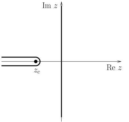
Qualitatively, it is the branch-point singularity that determines the form of $\mathcal{P}(N)$, and higher orders in perturbation theory, though leading to quantitative improvement, do not result in qualitative changes of that from. To get the asymptotic expansion of $\mathcal{P}(N)$, we deform the contour of the complex integral in Eq. (15) as illustrated in Fig. 2. If $\operatorname{Disc}\Phi$ denotes the discontinuity of the function $\Phi$ at the branch cut, we get

The non-universal factor $q\mathrm{e}^{z_{c}N+q\Phi(z_{c})}$ is common to all the quantities described by Eq. (6) and cancels therefore in all averages $\langle\mathcal{O}\rangle_{N}$. Note that for large $N$ only the small neighborhood of $z_{c}$ matters. In mean-field theory, it is easy to calculate $\mathcal{P}(N)$ without further approximation. We obtain

This distribution has its maximum near the characteristic value $N=N_{0}=q/r$. As stated above, we are, however, mainly interested in the rare events with $N\gg N_{0}$ where the asymptotic forms are valid. Note that the second line which gives the large-$N$ behavior is in perfect agreement with the well known asymptotic result $\mathcal{P}^{(\text{mf})}(N)\sim N^{-\theta^{(\text{mf})}}\exp(-N/N_{\infty}^{(\text{mf})})$ with the so-called entropic exponent given in mean-field approximation by $\theta^{(\text{mf})}=3/2$ and a non-universal number $N_{\infty}^{(\text{mf})}=2g/r^{2}$.

Gaussian fluctuations are governed by the second variations of the stochastic functional $\mathcal{J}_{z}$. After Fourier transformation in space and time, we have

where $c=c_{1}+c_{2}$. $\Gamma_{2,0;\rm{mf}}=-g\left.n\right|_{SP}$ is zero. The propagator follows from the inverse of $\Gamma_{1,1;\rm{mf}}$ in $(\mathbf{q},t)$-representation as

and the $\tilde{n}$-correlation function integrated over space and time is

The second virial coefficient follows from Eq. (14) to leading order as

It vanishes at the mean-field collapse transition, that is for $g^{\prime}r/g=0$.

Next, we calculate the average monomer density $\langle n(\bm{{\rm x}},t)\rangle_{N}$ emanating from a source at $(\bm{{\rm 0}},0)$. For this calculation, we recall Eq. (6). When specialized to $\mathcal{O}[n,\tilde{n}]=n(\bm{{\rm x}},t)$, the second line of Eq. (6) is equal to the Laplace transform of $\langle n(\mathbf{x},t)\tilde{n}(\mathbf{0},0)\rangle_{z}$ the latter being the (space-wise) Fourier transform of $G_{1,1}(\mathbf{q},t;z)$, Eq. (22). Collecting, we find that $\langle n(\bm{{\rm q}},t)\rangle_{N}$ can be written as

where the integration path is taken appropriately as outlined above for the probability distribution. The momentum integration back to the $(\mathbf{x},t)$ representation is straightforward, and we obtain

Form this result, we can read off directly that the longitudinal and transversal radii of gyration scale as $R_{\parallel}\sim N^{\nu_{A,\parallel}^{(\rm{mf})}}$ and $R_{\perp}\sim N^{\nu_{A,\perp}^{(\rm{mf})}}$ with the well known mean-field animal exponents

The response functional $\mathcal{J}_{z}=\mathcal{J}_{\rm{DP}}+z\mathcal{M}$, Eq. (16), is form-invariant under three continuous transformations. Thus, three parameters of the functional are redundant. Here, we exploit the symmetries to eliminate two redundant parameters and to define scale-invariant effective couplings.

The symmetry transformations are: (i) a rescaling of the fields

We eliminate the redundant parameters $r$ and $c$ by specializing the latter two, which do not transform the density field $n$, by

This special shift reminds of the saddle-point, Eq. (18b), and eliminates the uncritical parameter $r$ in favor of $\tau$. After this shift the fields and their expectation values are small quantities for small $\tau$, and a perturbation expansion is appropriate. The parameter $\tau$ is a free parameter at this place, and, of course, we can set this parameter to zero. However, it is more economical to use it in the renormalization program as a small control parameter because it attains at least an additive renormalization. The shift alone introduces besides the bilinear gradient term $\sim\tilde{n}\nabla^{2}n$ a further quadratic gradient term $\sim n\nabla^{2}n$ that is thereafter eliminated by the special mixing in Eq. (29). This term also attains renormalizations, and to cure UV-divergencies a counter term $\sim n\nabla^{2}n$ must be reintroduced via the renormalization scheme, which we will do as we proceed.

The transformation (29) suggests the definitions of new coupling constants

and new control parameters

Note that the three control parameters $\hat{\tau}_{0}$, $\hat{\tau}_{1}$, and $\hat{h}$ go to zero in the mean-field theory of the collapse of large branched polymers, i.e., near $z_{c}$, and that, however, the coupling constant $g_{1}$ stays finite.

The elimination of all terms that are at least irrelevant (in the sense of a naive scaling consideration) in comparison to the retained ones reduces the stochastic functional to

At this place we remark that for $g_{2}=0$ the stochastic functional $\mathcal{J}_{z}^{\prime}$ has the same form as the stochastic functional for ordinary directed percolation with a quadratic rapidity-reversal symmetry breaking $\sim\hat{\tau}_{1}$. Thus, in this special case the collapse transition belongs to the DP-universality class. Hence, we want to show wether $g_{2}$ is a relevant perturbation or it goes to zero under renormalization.

The modifications of the dynamical functional including the elimination of the irrelevant higher order couplings make it worthwhile to discuss the support of the functional integration over the fields $\tilde{n}$ and $n$ anew. Like before, the integration of $n$, the density of monomers, goes along the positive real axes. We write the third order terms of the integrand of $\mathcal{J}_{z}$ as

This form shows that the support of integration of $\tilde{n}$ must be so that $\tilde{n}-g_{1}n/2g_{0}$ is imaginary if this variable becomes large. The convergence of the functional integral then requires

to make sense beyond perturbation theory. If these conditions are violated, higher order contributions become relevant for stability reasons, and a first-order transition takes place. Next, we consider the quadratic terms of $\mathcal{J}^{\prime}_{z}$. Writing these terms as

we see that we have to require

for stability of the saddle-point at $\tilde{n}=n=0$ (for $\hat{h}=\hat{h}_{c}=0$). If these conditions are violated, a phase transition takes place.

Through the $\delta$-function condition in Eq. (7) which selects from all the generated clusters only the clusters with given mass $N$, the stochastic functional $\mathcal{J}^{\prime}_{z}$ has lost its typical causal structure, whereas the absorbing state condition still holds, $\mathcal{J}^{\prime}_{z}[\tilde{n},n=0]=0$. To restore the causal structure, we perform the duality transformation

These steps lead us from Eq. (32) to

Evidently, this new functional obeys causality, $\mathcal{J}[\tilde{\varphi}=0,\varphi]=0$, but the absorbing state property is satisfied only if $h=\tau_{1}=g_{2}=0$. If only $g_{2}=0$ holds, it defines RFT with added linear and quadratic symmetry breaking terms. In the following, two facts will play an important role: (i) RFT is equivalent to ordinary DP, and (ii) the added symmetry breaking terms do not alter the fixed point structure of RFT.

As it stands, the $\mathcal{J}$ is a truly proper field theoretic stochastic functional in the sense of being a minimal model. Nevertheless, it still contains that much generality that allows to study the statistics of swollen DBP and the CDBP transition. These will be the subjects of the following sections.

Our response functional $\mathcal{J}$, Eq. (38), describes specifically the CDBP transition when both control parameters $\hat{\tau}_{0}$ and $\hat{\tau}_{1}$ become critical. In this case, they scale in terms of the inverse length scale $\mu$ as $\hat{\tau}_{0}\sim\hat{\tau}_{1}\sim\mu^{2}$. Then the engineering dimensions of the fields and the remaining parameters follow as

Now, the upper critical dimension is $d_{c}=4$. All three coupling constants are relevant below $d_{c}$. There are no further contributions that are relevant under the condition of causality (originating from the absorbing condition of the process) which we have restored through the duality transformation (37).

It is well known that a perturbation expansion of correlation and response functions (generally called Greens functions) based on a field theoretic model like $\mathcal{J}$ produces UV-singularities which have to be regularized and renormalized by singular counter terms. Here, we use minimal renormalization, i.e., dimensional regularization followed by minimal subtraction of $\varepsilon$-poles, to cure the theory from UV-divergencies. For the general principles and methods of renormalization theory see, e.g., Ref. [40, 41].

In the following, we use a ring $\mathring{}$ to mark bare (unrenormalized) quantities, i.e., we let $\varphi\rightarrow\mathring{\varphi}$, and so on. From here on, quantities without a ring are understood as renormalized quantities. To get rid of $\varepsilon$-poles, we use the renormalization scheme

where $\varepsilon=4-d$ and $G_{\varepsilon}=\Gamma(1+\varepsilon/2)/(4\pi)^{d/2}$. Here, we have introduced the two-dimensional vector $\underline{\hat{\tau}}=(\hat{\tau}_{0},\hat{\tau}_{1})$. Note that the mixing-term proportional to $K$ reintroduces the aforementioned gradient term, see the discussion below Eq. (29). In minimal renormalization with dimensional expansion the additive contributions $\underline{\mathring{\hat{\tau}}}_{c}$, $\mathring{\hat{h}}_{c}$, $\underline{\mathring{C}}$ become formally zero, and the $\varepsilon$-content of the other counterterms are defined by pure Laurent-series:

where the counterterms $Y_{..}^{(l,k)}$, when determined at the loop-order $l$, are homogeneous polynomials of the renormalized dimensionless coupling constants $u_{\alpha}$ of order $2l$: $Y_{..}^{(l,k)}(su_{\alpha})=s^{2l}Y_{..}^{(l,k)}(u_{\alpha})$. Corresponding expansions are valid for the various other counterterms $K$, $\underline{\underline{A}}$, $B_{\alpha}$ which themselves are homogeneous polynomials of order $2l$, $2l-1$, $2l+1$, respectively, at each loop-order $l$. We calculate the various renormalization factors $Z_{..}$ and additional counter-terms using a two-tiered approach, viz. we carry out an explicit 1-loop calculation and we employ Ward identities. The latter will be discussed further below. Our 1-loop calculation, see the Appendix for details, produces

References

- [1] For a review see: L. Schäfer, Excluded Volume Effects in Polymer Solutions (Springer-Verlag, Berlin, Heidelberg, 1999) and the publications cited in this book.
- [2] H.-P. Hsu and P. Grassberger, J. Stat. Mech., P06003 (2005).
- [3] B. Derrida and H.J. Herrmann, J. Physique 44, 1365 (1983).
- [4] M. Henkel and F. Seno, Phys. Rev. E 53, 3662 (1996).
- [5] F. Seno and C. Vanderzande, J. Phys. A: Math. Gen. 27, 5813, 7937 (1994).
- [6] S. Flesia, D.S. Gaunt, C.E. Soteros and S.G. Whittington, J. Phys. A: Math. Gen. 25, L1169 (1992); 27, 5831 (1994) .
- [7] E.J. Janse van Rensburg et al., J. Phys. A: Math. Gen. 30, 8035 (1997); 32, 1567 (1999); 33, 3653 (2000).
- [8] S. Redner and A. Coniglio, J. Phys. A: Math. Gen. 15, L273 (1982).
- [9] D. Dhar, J. Phys. A: Math. Gen. 20, L847 (1987).
- [10] M. Knežević and J. Vannimenus, J. Phys. A: Math. Gen. 35, 2725 (2002).
- [11] J.Z. Imbrie, J. Phys. A: Math. Gen. 37, L137 (2004).
- [12] T.C. Lubensky and J. Isaacson, Phys. Rev. Lett. 41, 829 (1978), Phys. Rev. Lett. 42, 410(E) (1978), Phys. Rev. A 20, 2130 (1979).
- [13] A.B. Harris and T.C. Lubensky, Phys. Rev. B 23, 3591 (1981), Phys. Rev. B 24, 2656 (1981).
- [14] H. K. Janssen and O. Stenull, unpublished.
- [15] H.K. Janssen, Z. Phys. B 23, 377 (1976); R. Bausch, H.K. Janssen, and H. Wagner, Z. Phys. B 24, 113 (1976).
- [16] C. DeDominicis, J. Physique C 37, 247 (1976); C. DeDominicis and L. Peliti, Phys. Rev. B 18, 353 (1978).
- [17] H.K. Janssen, in: Dynamical Critical Phenomena and Related Topics, Lecture Notes in Physics, Vol. 104, ed. C.P. Enz (Springer, Heidelberg, 1979); H.K. Janssen, in: From Phase Transition to Chaos, eds. G. Györgyi, I. Kondor, L. Sasvári, T. Tél (World Scientific, Singapore, 1992).
- [18] For a recent review on the field theory approach to percolation processes see: H.K. Janssen and U.C. Täuber, Ann. Phys. (N.Y.) 315, 147 (2005).
- [19] D. Stauffer and A. Aharony, Introduction in Percolation Theory, 2nd ed. (Taylor and Francis, London 1992).
- [20] H.K. Janssen, Z. Phys. B: Cond. Mat. 42, 151 (1981).
- [21] H.K. Janssen, J. Stat. Phys. 103, 801 (2001).
- [22] T. Ohtsuki and T. Keyes, Phys. Rev. A 35, 2697 (1987); Phys. Rev. A 36, 4434 (1987).
- [23] H.K. Janssen, J. Phys. A: Math. Gen. 20, 5733 (1987).
- [24] H.K. Janssen, M. Müller, and O. Stenull, Phys. Rev. E 70, 026114 (2004).
- [25] H.K. Janssen, J. Phys. C: Cond. Mat. 17, S1973 (2005).
- [26] S. Lübeck, J. Stat. Phys. 123, 193 (2006).
- [27] M. Henkel, H. Hinrichsen, and S. Lübeck, Non-Equilibrium Phase Transitions, Vol. I: Absorbing Phase Transitions (Springer, Dordrecht, 2008).
- [28] U.C. Täuber, M.J. Howard, and B.P. Vollmayr-Lee, J. Phys. A: Math. Gen. 38, R79 (2005).
- [29] P. Grassberger, J. Stat. Mech. P01004, (2006) .
- [30] M. Ciafaloni and E. Onofri, Nucl. Phys. B 151, 118 (1979).
- [31] N. Breuer and H.K. Janssen, Z. Phys. B: Cond. Mat. 41, 55 (1981).
- [32] M.E. Fisher, Phys. Rev. Lett. 40, 1610 (1978).
- [33] N. Breuer and H.K. Janssen, Z. Phys. B: Cond. Mat. 48, 347 (1982).
- [34] J.L. Cardy, J. Phys. A: Math. Gen. 15, L593 (1982).
- [35] A.R. Day and T.C. Lubensky, J. Phys. A: Math. Gen. 15, L285 (1982).
- [36] J.L. Cardy, Phys. Rev. Lett. 54, 1354 (1985).
- [37] O.F. de Alcantara Bonfim, J.E. Kirkham, and A.J. McKane, J. Phys. A: Math. Gen. 14, 2391 (1981).
- [38] N. Breuer, Z. Phys. B: Cond. Mat. 54, 169 (1984).
- [39] S.-N. Lai and M.E. Fisher, J. Chem. Phys. 103, 8144 (1995).
- [40] D.J. Amit, Field Theory, the Renormalization Group, and Critical Phenomena (World Scientific, Singapore, 1984).
- [41] J. Zinn-Justin, Quantum Field Theory and Critical Phenomena (Clarendon, Oxford, fourth edition, 2002).
- [42] See, e.g., H. Wegner in: Phase Transitions and Critical Phenomena, Vol. 6, eds. C. Domb and J.L. Lebowitz (Academic Press, London, 1976).
- [43] H.K. Janssen, Ü. Kutbay, and K. Oerding, J. Phys. A: Math. Gen. 32, 1809 (1999).
- [44] See, e.g.,I.D. Lawrie and S. Sarbach in: Phase Transitions and Critical Phenomena, Vol. 9, eds. C. Domb and J.L. Lebowitz (Academic Press, London, 1984).
- [45] H. Hinrichsen, Adv. Phys. 49, 815 (2001).
- [46] S. Coleman, Phys. Rev. D 15, 2029 (1977); C.G. Callan and S. Coleman, Phys. Rev. D 16, 1792 (1977).
- [47] T.C. Lubensky and A.J. McKane, J. Phys. A: Math. Gen. 14, L157 (1981).
- [48] J.S. Langer, Ann. Phys. (N.Y.) 41, 108 (1967).
- [49] V. Alessandrini, D. Amati, and M. Ciafaloni, Nucl. Phys. B 130, 429 (1977).
- [50] N.J. Günther, D.A. Nicole, and D.J. Wallace, J. Phys. A: Math. Gen. 13, 1755 (1980).