跳到论文正文
W Papers独立论文阅读器 arXiv:0907.3372 论文正文 计算阅读时间 · 0%
引用这篇论文根据当前论文元数据生成,正式投稿前建议核对。


License: arXiv.org perpetual non-exclusive license
arXiv:0907.3372v2 [math.DS] 30 Dec 2009

SRB Measures for Certain Markov Processes

Wael Bahsoun Address: Department of Mathematical Sciences, Loughborough University, Loughborough, Leicestershire, LE11 3TU, UK Email address: W.Bahsoun@lboro.ac.uk and Paweł Góra Address: Department of Mathematics and Statistics, Concordia University, Montreal, Quebec, H3G 1M8, Canada Email address: pgora@mathstat.concordia.ca
Abstract.

We study Markov processes generated by iterated function systems (IFS). The constituent maps of the IFS are monotonic transformations of the interval. We first obtain an upper bound on the number of SRB (Sinai-Ruelle-Bowen) measures for the IFS. Then, when all the constituent maps have common fixed points at 0 and 1, theorems are given to analyze properties of the ergodic invariant measures δ0\delta_{0} and δ1\delta_{1}. In particular, sufficient conditions for δ0\delta_{0} and/or δ1\delta_{1} to be, or not to be, SRB measures are given. We apply some of our results to asset market games.

Key words and phrases: 
Iterated Function System, SRB-Measures
1991 Mathematics Subject Classification
Primary 37A05, 37E05, 37H99

1. Introduction

In the 1970’s, Sinai, Ruelle and Bowen studied the existence of an important class of invariant measures in the context of deterministic dynamical systems. These invariant measures are nowadays known as SRB (Sinai-Ruelle-Bowen) measures [14]. SRB measures are distinguished among other ergodic invariant measures because of their physical importance. In fact, from ergodic theory point of view, they are the only useful ergodic measures. This is due to the fact that SRB measures are the only ergodic measures for which the Birkhoff Ergodic Theorem holds on a set of positive measure of the phase space. In this note, we study SRB measures in a stochastic setting—Markov processes generated by iterated function systems (IFS).

An IFS11 1 In some of the literature an IFS is called a random map or a random transformation. is a discrete-time random dynamical system [1, 10] which consists of a finite collection of transformations and a probability vector {τs;ps}s=1L\{\tau_{s};p_{s}\}_{s=1}^{L}. At each time step, a transformation τs\tau_{s} is selected with probability ps>0p_{s}>0 and applied to the process. IFS has been a very active topic of research due to its wide applications in fractals and in learning models. The survey articles [5, 13] contain a considerable list of references and results in this area.

The systems which we study in this note do not fall in the category of the IFS22 2 In most articles about IFS, the constituent maps are assumed to be contracting or at least contracting on average. Here we do not impose any assumption of this type. In fact the class of IFS which we study in Section 4 cannot satisfy such assumptions. considered in [5, 13] and references therein. Moreover, in general, our IFS do not satisfy the classical splitting33 3 In particular, when all the maps have common fixed points at 0 and 1. See Section 4. condition of [7]. In fact, our aim in this note is to depart from the traditional goal of finding sufficient conditions for an IFS to admit a unique attracting invariant measure [7, 5, 13]. Instead, we study cases where an IFS may admit more than one invariant measure and aim to identify the physically relevant ones; i.e., invariant measures for which the Ergodic Theorem holds on a set of positive measure of the ambient phase space. We call such invariant measures SRB.

Physical SRB measures for random maps have been studied by Buzzi [3] in the context of random Lasota-Yorke maps. However, Buzzi’s definition of a basin of an SRB measure is different from ours. We will clarify this difference in Section 2. A general concept of an SRB measure for general random dynamical systems can be found in the survey article [11]. In this note we study physical SRB measures for IFS whose constituent maps are strictly increasing transformations of the interval. We obtain an upper bound on the number of SRB measures for the IFS. Moreover, when all the constituent maps have common fixed points at 0 and 1, we provide sufficient conditions for δ0\delta_{0} and/or δ1\delta_{1} to be, or not to be, SRB measures. To complement our theoretical results, we show at the end of this note that examples of IFS of this type can describe evolutionary models of financial markets [4].

In Section 2 we introduce our notation and main definitions. In particular, Section 2 includes the definition of an SRB measure for an IFS. In Section 3 we identify the structure of the basins of SRB measures and we obtain a sharp upper bound on the number of SRB measures. Section 4 contains sufficient conditions for δ0\delta_{0} and δ1\delta_{1}, the delta measures concentrated at 00 and 11 respectively, to be SRB. It also contains sufficient conditions for δ0\delta_{0} and δ1\delta_{1} not to be SRB measures. Our main results in this section are Theorems 4.3 and Theorem 4.7. In Section 5 we study ergodic properties of δ0\delta_{0} and δ1\delta_{1} without having any information about the probability vector of the IFS. In Section 6 we apply our results to asset market games. In particular, we find a generalization of the famous Kelly rule [9] which expresses the principle of “betting your beliefs”. The importance of our generalization lies in the fact that it does not require the full knowledge of the probability distribution of the random states of the system. Section 7 contains an auxiliary result which we use in the proof of Theorem 4.7.

2. Preliminaries

2.1. Notation and assumptions

Let ([0,1],𝔅)([0,1],\mathfrak{B}) be the measure space where 𝔅\mathfrak{B} is the Borel σ\sigma-algebra on [0,1][0,1]. Let λ\lambda denote Lebesgue measure on ([0,1],𝔅)([0,1],\mathfrak{B}) and δr\delta_{r} denote the delta measure concentrated at point r∈[0,1]r\in[0,1]. Let S={1,…,L}S=\{1,\dots,L\} be a finite set and τs\tau_{s}, s∈Ss\in S, be continuous transformations from the unit interval into itself. We assume:

(A) τs\tau_{s} are strictly increasing.

Let 𝐩=(ps)s=1L\mathbb{\bf p}=(p_{s})_{s=1}^{L} be a probability vector on SS such that for all s∈Ss\in S, ps>0p_{s}>0. The collection

F={τ1,τ2,…,τL;p1,p2,…,pL}F=\{\tau_{1},\tau_{2},\dots,\tau_{L};p_{1},p_{2},\dots,p_{L}\}

is called an iterated function system (IFS) with probabilities.

We denote the space of sequences ω={s1,s2,…}\omega=\{s_{1},s_{2},\dots\}, sl∈Ss_{l}\in S, by Ω\Omega. The topology on Ω\Omega is defined as the product of the discrete topologies on SS. Let π𝐩\pi_{\bf p} denote the Borel measure on Ω\Omega defined as the product measure 𝐩ℕ{\bf p}^{\mathbb{N}}. Moreover, we write

st:=(s1,s2,…,st)s^{t}:=(s_{1},s_{2},\dots,s_{t})

for the history up to time tt, and for any r0∈[0,1]r_{0}\in[0,1] we write

rt(st):=τst∘τst−1∘⋯∘τs1(r0).r_{t}(s^{t}):=\tau_{s_{t}}\circ\tau_{s_{t-1}}\circ\cdots\circ\tau_{s_{1}}(r_{0}).

Finally, by E⁡(⋅)E(\cdot) we denote the expectation with respect to 𝐩\bf{p}, by E(⋅|st)E(\cdot|s^{t}) the conditional expectation given the history up to time tt and by var⁡(⋅){\rm var}(\cdot) the variance with respect to 𝐩\bf{p}.

2.2. Invariant measures

FF is understood as a Markov process with a transition function

ℙ⁡(r,A)=∑s=1Lps​χA​(τs​(r)),\mathbb{P}(r,A)=\sum_{s=1}^{L}p_{s}\chi_{A}(\tau_{s}(r)),

where A∈𝔅A\in\mathfrak{B} and χA\chi_{A} is the characteristic function of the set AA. The transition function ℙ\mathbb{P} induces an operator PP on measures on ([0,1],𝔅)([0,1],\mathfrak{B}) defined by

(2.1) P​μ​(A)=∫01ℙ⁡(r,A)​dμ​(r)=∑s=1Lps​μ​(τs−1​A).\begin{split}P\mu(A)&=\int_{0}^{1}\mathbb{P}(r,A)d\mu(r)\\ &=\sum_{s=1}^{L}p_{s}\mu(\tau^{-1}_{s}A).\\ \end{split}

Following the standard notion of an invariant measure for a Markov process, we call a probability measure μ\mu on ([0,1],𝔅)([0,1],\mathfrak{B}) FF-invariant probability measure if and only if

P​μ=μ.P\mu=\mu.

Moreover, it is called ergodic if it cannot be written as a convex combination of other invariant probability measures.

2.3. SRB measures

Let μ\mu be an ergodic probability measure for the IFS. Suppose there exists a set of positive Lebesgue measure in [0,1][0,1] such that

(2.2) 1T​∑t=0T−1δrt​(st)​→weakly​μwith ​π𝐩​-probability one.\frac{1}{T}\sum_{t=0}^{T-1}\delta_{r_{t}(s^{t})}\overset{\text{weakly}}{\to}\mu\hskip 28.45274pt\text{with }\pi_{\bf p}\text{-probability one.}

Then μ\mu is called an SRB (Sinai-Ruelle-Bowen) measure. The set of points r0∈[0,1]r_{0}\in[0,1] for which (2.2) is satisfied will be called the basin44 4 Our definition of a basin is different from Buzzi’s definition [3]. In his definition he defines random basins Bω​(μ)B_{\omega}(\mu) for an SRB measure. In particular, according to Buzzi’s definition, for the same SRB measure, basins corresponding to two different ω\omega’s may differ on a set of positive lebsegue measure of [0,1][0,1]. See [3] for more detials. of μ\mu and it will be denoted by B⁡(μ)B(\mu). Obviously, if λ⁡(B⁡(μ))=1\lambda(B(\mu))=1 then μ\mu is the unique SRB measure of FF.

3. Number of SRB measures and their basins

The basin of an SRB measure for the systems we are dealing with is described by the following two propositions.

Proposition 3.1.

Let μ\mu be an SRB measure and B⁡(μ)B(\mu) be its basin. Let r0,r¯0∈B⁡(μ)r_{0},\bar{r}_{0}\in B(\mu), r0>r¯0r_{0}>\bar{r}_{0}. Then [r¯0,r0]⊆B⁡(μ)[\bar{r}_{0},r_{0}]\subseteq B(\mu).

Proof.

When weak convergence is considered on an interval, then μn​→weakly​μ\mu_{n}\overset{\text{weakly}}{\to}\mu if and only if μn​(f)→μ​(f)\mu_{n}(f)\to\mu(f) for any C1C^{1} function55 5 Here is a sketch of the proof of this claim: Assume μn​(f)→μ​(f)\mu_{n}(f)\to\mu(f)\, for any f∈C1​([0,1])f\in C^{1}([0,1]). Let gg be a continuous function and let {fk}k≥1\{f_{k}\}_{k\geq 1} be a sequence of C1C^{1} functions converging to gg in C0C^{0} norm. We have |μn​(g)−μ​(g)|≤|μn​(g)−μn​(fk)|+|μn​(fk)−μ⁡(fk)|+|μ⁡(fk)−μ⁡(g)|≤2​‖fk−g‖C0+|μn​(fk)−μ⁡(fk)|.\begin{split}|\mu_{n}(g)-\mu(g)|&\leq|\mu_{n}(g)-\mu_{n}(f_{k})|+|\mu_{n}(f_{k})-\mu(f_{k})|+|\mu(f_{k})-\mu(g)|\\ &\leq 2\|f_{k}-g\|_{C^{0}}+|\mu_{n}(f_{k})-\mu(f_{k})|\ .\end{split} Now, for any ε>0\varepsilon>0, we can find k0k_{0} such that 2​‖fk0−g‖C0<ε/22\|f_{k_{0}}-g\|_{C^{0}}<\varepsilon/2 and then we can find n0n_{0} such that for any n≥n0n\geq n_{0} we have |μn​(fk0)−μ⁡(fk0)|<ε/2|\mu_{n}(f_{k_{0}})-\mu(f_{k_{0}})|<\varepsilon/2.. Since every C1C^{1} function is a difference of two continuous increasing functions, this means that μn​→weakly​μ\mu_{n}\overset{\text{weakly}}{\to}\mu if and only if μn​(f)→μ​(f)\mu_{n}(f)\to\mu(f) for any continuous increasing function.

Let r0,r¯0∈B⁡(μ)r_{0},\bar{r}_{0}\in B(\mu) and r¯0<r0′<r0\bar{r}_{0}<r^{\prime}_{0}<r_{0}. We will show that r0′∈B⁡(μ)r^{\prime}_{0}\in B(\mu). Let assume that ff is continuous and increasing. Let us fix an sts^{t} for which

limT→∞1T​∑t=0T−1f⁡(r¯t​(st))=limT→∞1T​∑t=0T−1f⁡(rt​(st))=μ⁡(f).\lim_{T\to\infty}\frac{1}{T}\sum_{t=0}^{T-1}f(\bar{r}_{t}(s^{t}))=\lim_{T\to\infty}\frac{1}{T}\sum_{t=0}^{T-1}f(r_{t}(s^{t}))=\mu(f).

We have r¯t​(st)<rt′​(st)<rt​(st)\bar{r}_{t}(s^{t})<r^{\prime}_{t}(s^{t})<r_{t}(s^{t}) (since all τs\tau_{s} are increasing) and

1T​∑t=0T−1f⁡(r¯t​(st))≤1T​∑t=0T−1f⁡(rt′​(st))≤1T​∑t=0T−1f⁡(rt​(st)).\frac{1}{T}\sum_{t=0}^{T-1}f(\bar{r}_{t}(s^{t}))\leq\frac{1}{T}\sum_{t=0}^{T-1}f(r^{\prime}_{t}(s^{t}))\leq\frac{1}{T}\sum_{t=0}^{T-1}f(r_{t}(s^{t})).

The averages on the left and on the right have common limit μ⁡(f)\mu(f). Thus,

1T​∑t=0T−1δrt′​(st)​(f)=1T​∑t=0T−1f⁡(rt′​(st))→μ⁡(f).\frac{1}{T}\sum_{t=0}^{T-1}\delta_{r^{\prime}_{t}(s^{t})}(f)=\frac{1}{T}\sum_{t=0}^{T-1}f(r^{\prime}_{t}(s^{t}))\to\mu(f).

Since the event

{limT→∞1T∑t=0T−1f(r¯t(st))=limT→∞1T∑t=0T−1f(rt(st))=μ(f)}\{\lim_{T\to\infty}\frac{1}{T}\sum_{t=0}^{T-1}f(\bar{r}_{t}(s^{t}))=\lim_{T\to\infty}\frac{1}{T}\sum_{t=0}^{T-1}f(r_{t}(s^{t}))=\mu(f)\}

occurs with π𝐩\pi_{\bf p}-probability 1, the event

{1T∑t=0T−1f(rt′(st))→μ(f)}\{\frac{1}{T}\sum_{t=0}^{T-1}f(r^{\prime}_{t}(s^{t}))\to\mu(f)\}

also occurs with π𝐩\pi_{\bf p}-probability 1. ∎

Proposition 3.2.

Let μ\mu be an SRB measure and B⁡(μ)=⟨a,b⟩B(\mu)=\langle a,b\rangle be its basin, where ⟨a,b⟩\langle a,b\rangle denotes an interval closed or open at any of the endpoints. Then,

τs​(a)≥a,s=1,…,L,and if 
​a
≠0
then 
​τs​(a)
=a
for at least one ​s
;
\tau_{s}(a)\geq a\ \ ,\ \ s=1,\dots,L,\ \ \text{and if }\\ a\not=0\ \ \text{then }\\ \tau_{s}(a)=a\ \ \text{for at least one }s;
τs​(b)≤b,s=1,…,L,and if 
​b
≠1
then τs​(b)=bfor at least one ​s
.
\tau_{s}(b)\leq b\ \ ,\ \ s=1,\dots,L,\ \ \text{and if }\\ b\not=1\ \ \text{then }\ \ \tau_{s}(b)=b\ \ \text{for at least one }s.
Proof.

We will prove only the second claim with b≠1b\not=1. The first claim is proven analogously.

Assume that τs0​(b)>b\tau_{s_{0}}(b)>b, for some 1≤s0≤L1\leq s_{0}\leq L. Then, we can find r0∈(a,b)r_{0}\in(a,b) such that τs0​(r0)>b\tau_{s_{0}}(r_{0})>b. For arbitrary continuous function ff, for ω∈A⊂Ω\omega\in A\subset\Omega with π𝐩​(A)=1\pi_{\bf p}(A)=1, we have

limT→∞1T​∑t=0T−1f⁡(rt​(st))=μ⁡(f).\lim_{T\to\infty}\frac{1}{T}\sum_{t=0}^{T-1}f(r_{t}(s^{t}))=\mu(f).

The set As0={(s1,s2,…):(s0,s1,s2,…)∈A}A_{s_{0}}=\{(s_{1},s_{2},\dots):(s_{0},s_{1},s_{2},\dots)\in A\} is also of π𝐩\pi_{\bf p}-probability 1. Let r0′=τs0​(r0)r^{\prime}_{0}=\tau_{s_{0}}(r_{0}) and let (st)′(s^{t})^{\prime} denote the initial subsequences of length tt of ω∈As0\omega\in A_{s_{0}} . Then,

1T​∑t=0T−1f⁡(rt′​((st)′))=1T​∑t=0T−1f⁡(rt​(st))−1T​f​(r0)+1T​f​(rT−1′​((sT−1)′))​⟶T→+∞​μ​(f).\frac{1}{T}\sum_{t=0}^{T-1}f(r^{\prime}_{t}((s^{t})^{\prime}))=\frac{1}{T}\sum_{t=0}^{T-1}f(r_{t}(s^{t}))-\frac{1}{T}f(r_{0})+\frac{1}{T}f(r^{\prime}_{T-1}((s^{T-1})^{\prime}))\underset{T\to+\infty}{\longrightarrow}\mu(f).

This shows that τs0​(r0)∈Bω​(μ)\tau_{s_{0}}(r_{0})\in B_{\omega}(\mu) and contradicts the assumptions.

Now, we assume that τs​(b)<b\tau_{s}(b)<b, s=1,…,Ls=1,\dots,L. Then, we can find r0>br_{0}>b such that τs​(r0)∈(a,b)\tau_{s}(r_{0})\in(a,b) for all ss. Let

As={ω:limT→∞1T∑t=0T−1f(rt′(st))=μ(f),forr0′=τs(r0)},s=1,…,L.A_{s}=\{\omega:\lim_{T\to\infty}\frac{1}{T}\sum_{t=0}^{T-1}f(r^{\prime}_{t}(s^{t}))=\mu(f),\ \text{for}\ r^{\prime}_{0}=\tau_{s}(r_{0})\}\ ,\ s=1,\dots,L\ .

We have π𝐩​(As)=1\pi_{\bf p}(A_{s})=1 for each ss. Hence, π𝐩​(A)=1\pi_{\bf p}(A)=1, where A=∪1≤s≤L(s,As)A=\cup_{1\leq s\leq L}(s,A_{s}) and (s,As)={(s,s1,s2,s3,…):(s1,s2,s3,…)∈As}(s,A_{s})=\{(s,s_{1},s_{2},s_{3},\dots):(s_{1},s_{2},s_{3},\dots)\in A_{s}\}. For arbitrary continuous function ff, for ω∈A\omega\in A, if ω1=s\omega_{1}=s we have

limT→∞1T​∑t=0T−1f⁡(rt​(st))=limT→∞(1T​∑t=0T−1f⁡(rt′​((st)′))+1T​f​(r0)−1T​f​(rT−1′​((sT−1)′)))=μ⁡(f),\begin{split}&\lim_{T\to\infty}\frac{1}{T}\sum_{t=0}^{T-1}f(r_{t}(s^{t}))\\ &=\lim_{T\to\infty}\left(\frac{1}{T}\sum_{t=0}^{T-1}f(r^{\prime}_{t}((s^{t})^{\prime}))+\frac{1}{T}f(r_{0})-\frac{1}{T}f(r^{\prime}_{T-1}((s^{T-1})^{\prime}))\right)=\mu(f),\end{split}

where r0′=τs​(r0)r^{\prime}_{0}=\tau_{s}(r_{0}) and (st)′(s^{t})^{\prime} are the initial subsequences of length tt of ω∈As\omega\in A_{s}. This implies that r0∈B⁡(μ)r_{0}\in B(\mu). Since r0>br_{0}>b, this leads to a contradiction. ∎

We now state the main result of this section. Firstly, we recall that ⟨⋅,⋅⟩\langle\cdot,\cdot\rangle denotes an interval which is closed or open at any of the endpoints. Secondly, we define a set BS whose elements are intervals of the form ⟨⋅,⋅⟩\langle\cdot,\cdot\rangle with the following property:

⟨a,b⟩∈BS\langle a,b\rangle\in\textbf{BS}

if and only if

τs​(a)≥a,s=1,…,Landτs​(a)=afor at least one ​s;\tau_{s}(a)\geq a\ \ ,\ \ s=1,\dots,L\ \ \text{and}\ \ \tau_{s}(a)=a\ \ \text{for at least one }s;

and

τs​(b)≤b,s=1,…,Landτs​(b)=bfor at least one ​s.\tau_{s}(b)\leq b\ \ ,\ \ s=1,\dots,L\ \ \text{and}\ \ \tau_{s}(b)=b\ \ \text{for at least one }s.
Theorem 3.3.

The number of SRB measures of FF is bounded above by the cardinality of the set BS. In particular, if 00 and 11 are the only fixed points of some τs0\tau_{s_{0}}, s0∈Ss_{0}\in S, then FF admits at most one SRB measure.

Proof.

The fact that number of SRB measures of FF is bounded above by the cardinality of the set BS is a direct consequence of Proposition 3.2. To elaborate on the second part of the theorem, assume without loss of generality that τs0​(r)>r\tau_{s_{0}}(r)>r for all r∈(0,1)r\in(0,1). Obviously, by Proposition 3.2, if all the other maps τs\tau_{s}, s∈S∖{s0}s\in S\setminus\{s_{0}\} has no fixed points in (0,1)(0,1), then FF admits at most one SRB measure. So let us assume that there exists an s∗∈S∖{s0}s^{*}\in S\setminus\{s_{0}\} such that τs∗\tau_{s^{*}} has a finite or infinite number of fixed points in [0,1][0,1]. In the case of finite number of fixed points, denote the fixed points of τs∗\tau_{s^{*}} in [0,1] by ri∗r^{*}_{i}, i=1,…,qi=1,\dots,q, such that 0≤r1∗<r2∗<⋯<rq∗≤10\leq r^{*}_{1}<r^{*}_{2}<\cdots<r^{*}_{q}\leq 1. Since τs​(ri∗)>ri∗\tau_{s}(r^{*}_{i})>r^{*}_{i} for all ri∗∈(0,1)r^{*}_{i}\in(0,1), the only possible basin for an SRB measure would be either ⟨rq−1∗,1⟩\langle r^{*}_{q-1},1\rangle or ⟨rq∗,1⟩\langle r^{*}_{q},1\rangle. In the case of infinite number of fixed points, let

r¯=sup{r∈(0,1):τs∗​(r)=r}.\bar{r}=\sup\{r\in(0,1):\,\tau_{s^{*}}(r)=r\}.

If r¯<1\bar{r}<1, then τs0​(r¯)>r¯\tau_{s_{0}}(\bar{r})>\bar{r}. By Proposition 3.2, ⟨r¯,1⟩\langle\bar{r},1\rangle is the only possible basin for an SRB measure. If r¯=1\bar{r}=1, let J¯\bar{J} denote the closure of the set of fixed points of τs∗\tau_{s^{*}} and let J¯0⊆J¯\bar{J}_{0}\subseteq\bar{J} be the minimal closed subset of J¯\bar{J} which contains the point 11. J¯0\bar{J}_{0} is the only possible basin for an SRB measure. Moreover, it cannot be decomposed into basins of different SRB measures. Indeed, let J1∪J2=J¯0J_{1}\cup J_{2}=\bar{J}_{0} such that J1=⟨a,b⟩J_{1}=\langle a,b\rangle with b<1b<1. Since τs0​(b)>b\tau_{s_{0}}(b)>b, by Proposition 3.2, J1J_{1} cannot be a basin of an SRB measure. Thus, FF admits at most one SRB measure. ∎

The following example shows that Proposition 3.2 can be used to identify intervals which are not in the basin of an SRB measure. In particular, it shows that the bound obtained on the number of SRB measures in Theorem 3.3 is really sharp.

Example 3.4.

Let

τ1​(r)={3​r2,for 0≤r≤1/3;1−32​(r−1)2,for 1/3<r≤1;,\tau_{1}(r)=\begin{cases}3r^{2}&,\ \text{for}\ \ 0\leq r\leq 1/3;\\ 1-\frac{3}{2}(r-1)^{2}&,\ \text{for}\ \ 1/3<r\leq 1;\end{cases}\ \ \ ,\ \ \

and

τ2​(r)={32​r2,for 0≤r≤2/3;1−3​(r−1)2,for 2/3<r≤1.\tau_{2}(r)=\begin{cases}\frac{3}{2}r^{2}&,\ \text{for}\ \ 0\leq r\leq 2/3;\\ 1-3(r-1)^{2}&,\ \text{for}\ \ 2/3<r\leq 1.\end{cases}

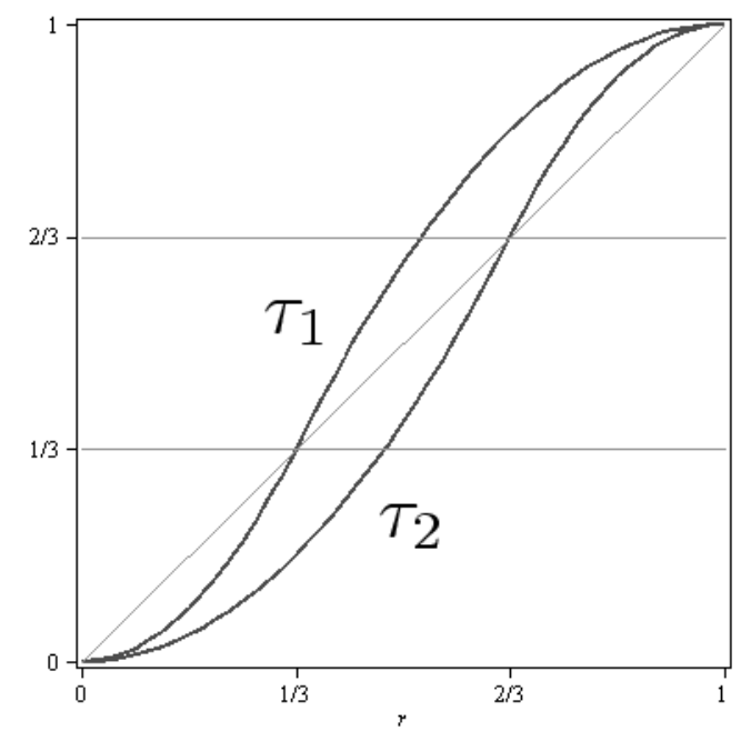
The graphs of the above maps are shown in Figure 1. Using Proposition 3.2, we see that the points of the interval (1/3,2/3)(1/3,2/3) do not belong to a basin of any SRB measure. Moreover, by Theorem 3.3, FF admits at most two SRB measures. Indeed, one can easily check that δ0\delta_{0} and δ1\delta_{1} are the only SRB measures with basins B⁡(δ0)=[0,1/3]B(\delta_{0})=[0,1/3] and B⁡(δ1)=[2/3,1]B(\delta_{1})=[2/3,1] respectively. For any r∈[0,1/3)r\in[0,1/3) for all ω\omega’s the averages 1T​∑t=0T−1δrt​(st)\frac{1}{T}\sum_{t=0}^{T-1}\delta_{r_{t}(s^{t})} converge weakly to δ0\delta_{0}. For r=1/3r=1/3 the only ω\omega for which this does not happen is ω={1,1,1,…}\omega=\{1,1,1,\dots\} so again the averages converge weakly to δ0\delta_{0} with π𝐩\pi_{\bf p}-probability 1. Similarly, we can show that B⁡(δ1)=[2/3,1]B(\delta_{1})=[2/3,1]. If r∈(1/3,2/3)r\in(1/3,2/3), then with positive π𝐩\pi_{\bf p}-probability the averages converge to δ0\delta_{0} and with positive π𝐩\pi_{\bf p}-probability the averages converge to δ1\delta_{1}. Thus, these points do not belong to a basin of any SRB measure and there are only two SRB measures.
Refer to caption
Figure 1. Maps τ1\tau_{1} and τ2\tau_{2} in Example 3.4

4. Properties of δ0\delta_{0} and δ1\delta_{1}

In addition to condition (A), we assume in this section that for all s∈Ss\in S:

(B) τs​(0)=0\tau_{s}(0)=0 and τs​(1)=1\tau_{s}(1)=1;

Obviously by Condition (B) the delta measures δ0\delta_{0} and δ1\delta_{1} are ergodic probability measures for the IFS. We will be mainly concerned with the following question: When does FF have δ0\delta_{0} and/or δ1\delta_{1} as SRB measures? We start our analysis by proving a lemma which provides a sufficient condition for δx\delta_{x}, the point measure concentrated at x∈[0,1]x\in[0,1], to be an SRB measure.

Lemma 4.1.

Suppose that τs​(x)=x\tau_{s}(x)=x for all s∈{1,…,L}s\in\{1,\dots,L\} and that there exists an initial point of a random orbit r0r_{0}, r0≠xr_{0}\not=x, for which limt→∞rt​(st)=x\lim_{t\to\infty}r_{t}(s^{t})=x with probability π𝐩=1\pi_{\bf p}=1. Then δx\delta_{x} is an SRB measure for FF and Bω​(δx)⊇[x,r0]B_{\omega}(\delta_{x})\supseteq[x,r_{0}]66 6 The notation here is for the case when r0>xr_{0}>x..

Proof.

Let ff be a continuous function on [0,1][0,1]. Let r0≠xr_{0}\not=x and fix a history sts^{t} for which limt→∞rt​(st)=x\lim_{t\to\infty}r_{t}(s^{t})=x. Then

limt→∞f⁡(rt​(st))=f⁡(x).\lim_{t\to\infty}f(r_{t}(s^{t}))=f(x).

Consequently

limT→∞1T​∑t=0T−1f⁡(rt​(st))=f⁡(x).\lim_{T\to\infty}\frac{1}{T}\sum_{t=0}^{T-1}f(r_{t}(s^{t}))=f(x).

Since the event

{limt→∞rt(st)=x}\{\lim_{t\to\infty}r_{t}(s^{t})=x\}

appears with probability one, the event

{limT→∞1T∑t=0T−1f(rt(st))=f(x)}\{\lim_{T\to\infty}\frac{1}{T}\sum_{t=0}^{T-1}f(r_{t}(s^{t}))=f(x)\}

also appears with probability one. Thus, by Proposition 3.1, δx\delta_{x} is an SRB measure for FF and Bω​(δx)⊇[x,r0]B_{\omega}(\delta_{x})\supseteq[x,r_{0}]. ∎

The following lemma, which is easy to prove, is a key observation for our main results in this section.

Lemma 4.2.

Each constituent map of the IFS can be represented as follows:

τs​(r)=rβs​(r),\tau_{s}(r)=r^{\beta_{s}(r)},

with βs​(r)\beta_{s}(r) satisfying:

  1. (1)

    βs​(r)>0\beta_{s}(r)>0 in (0,1)(0,1) ;

  2. (2)

    (ln⁡r)​βs​(r)(\ln r)\beta_{s}(r) increasing;

  3. (3)

    limr→0(ln⁡r)​βs​(r)=−∞\lim_{r\to 0}(\ln r)\beta_{s}(r)=-\infty;

  4. (4)

    limr→1(ln⁡r)​βs​(r)=0.\lim_{r\to 1}(\ln r)\beta_{s}(r)=0.

In the rest of this section, the following notation will be used:

αt:⁣=defβs(rt−1) with probability ps,t=1,2,…\alpha_{t}\overset{\text{def}}{:=}\beta_{s}(r_{t-1})\text{ with probability }p_{s},\,t=1,2,\dots
Theorem 4.3.

Let F={τs;ps}s∈SF=\{\tau_{s};p_{s}\}_{s\in S} be an IFS such that τs​(r)=rβs​(r)\tau_{s}(r)=r^{\beta_{s}(r)}. Assume that 0<bs≤βs​(r)≤Bs<∞0<b_{s}\leq\beta_{s}(r)\leq B_{s}<\infty for all r∈[0,1]r\in[0,1].

  1. (1)

    If E⁡(ln⁡αt|st−1)≤0E(\ln\alpha_{t}|s^{t-1})\leq 0 a.s., then limt→∞rt​(st)≠0\lim_{t\to\infty}r_{t}(s^{t})\not=0 a.s.

  2. (2)

    If lim supT→∞1T​∑t=1TE⁡(ln⁡αt|st−1)<0\limsup_{T\to\infty}\frac{1}{T}\sum_{t=1}^{T}E(\ln\alpha_{t}|s^{t-1})<0 a.s., then limt→∞rt​(st)=1\lim_{t\to\infty}r_{t}(s^{t})=1 a.s.

  3. (3)

    If lim infT→∞1T​∑t=1TE⁡(ln⁡αt|st−1)>0\liminf_{T\to\infty}\frac{1}{T}\sum_{t=1}^{T}E(\ln\alpha_{t}|s^{t-1})>0 a.s., then limt→∞rt​(st)=0\lim_{t\to\infty}r_{t}(s^{t})=0 a.s.

Proof.

Let us consider the sequence of random exponents

α(t)=αtαt−1⋯α2α1,\alpha(t)=\alpha_{t}\alpha_{t-1}\cdots\alpha_{2}\alpha_{1},

where αi=βs​(ri−1)\alpha_{i}=\beta_{s}(r_{i-1}) with probability psp_{s}, and observe that

rt​(st)=rα⁡(t).r_{t}(s^{t})=r^{\alpha(t)}.

We have

ln⁡α⁡(t+1)=ln⁡αt+1+ln⁡α⁡(t),\ln\alpha(t+1)=\ln\alpha_{t+1}+\ln\alpha(t),

and, with probability one,

E⁡(ln⁡α⁡(t+1)|st)−ln⁡(α⁡(t))=E⁡(ln⁡αt+1|st)≤0.E(\ln\alpha(t+1)|s^{t})-\ln(\alpha(t))=E(\ln\alpha_{t+1}|s^{t})\leq 0.

Therefore, ln⁡α⁡(t)\ln\alpha(t) is a supermartingale. Moreover, because 0<bs≤βs​(rt)≤Bs<∞0<b_{s}\leq\beta_{s}(r_{t})\leq B_{s}<\infty, |ln⁡α⁡(t+1)−ln⁡α⁡(t)|=|ln⁡αt+1|<∞|\ln\alpha(t+1)-\ln\alpha(t)|=|\ln\alpha_{t+1}|<\infty. Hence ln⁡α⁡(t)\ln\alpha(t) is a supermartingale with bounded increments. Thus, using Theorem 5.1 in Chapter VII of [12], with probability one ln⁡α⁡(t)\ln\alpha(t) does not converge to +∞+\infty. Consequently, with probability one, rt​(st)=rα⁡(t)r_{t}(s^{t})=r^{\alpha(t)} does not converge to zero.

We now prove the second statement of the theorem. Again we consider the sequence of random exponents

α(t)=αtαt−1⋯α2α1.\alpha(t)=\alpha_{t}\alpha_{t-1}\cdots\alpha_{2}\alpha_{1}.

Let MtM_{t} denote the martingale difference

Mt:=ln⁡αt−E⁡(ln⁡αt|st−1).M_{t}:=\ln\alpha_{t}-E(\ln\alpha_{t}|s^{t-1}).

We have E⁡(Mt)=0E(M_{t})=0 and ln⁡αt\ln\alpha_{t} is uniformly bounded. Therefore, by the strong law of large numbers (see Theorem 2.19 in [8]), with probability one

(4.1) limT→∞1T​∑t=1TMt=0.\lim_{T\to\infty}\frac{1}{T}\sum_{t=1}^{T}M_{t}=0.

Therefore, with probability one,

lim supT→∞1T​ln⁡α⁡(T)=lim supT→∞1T​∑t=1Tln⁡αt=lim supT→∞1T​∑t=1TMt+lim supT→∞1T​∑t=1TE⁡(ln⁡αt|st−1)<0.\begin{split}\limsup_{T\to\infty}\frac{1}{T}\ln\alpha(T)&=\limsup_{T\to\infty}\frac{1}{T}\sum_{t=1}^{T}\ln\alpha_{t}\\ &=\limsup_{T\to\infty}\frac{1}{T}\sum_{t=1}^{T}M_{t}+\limsup_{T\to\infty}\frac{1}{T}\sum_{t=1}^{T}E(\ln\alpha_{t}|s^{t-1})<0.\end{split}

From this we can conclude that for TT large enough there is a positive random variable η\eta such that

α⁡(T)≤e−T​η​ a.s.\alpha(T)\leq e^{-T\eta}\text{ a.s.}

Thus, since r∈[0,1]r\in[0,1], for TT large enough we obtain

rT+1=rα⁡(T)≥re−T​η​ a.s.r_{T+1}=r^{\alpha(T)}\geq r^{e^{-T\eta}}\text{ a.s.}

By taking the limit of TT to infinity we obtain

limT→∞rT+1=limT→∞rα⁡(T)≥limT→∞re−T​η=1​ a.s.\lim_{T\to\infty}r_{T+1}=\lim_{T\to\infty}r^{\alpha(T)}\geq\lim_{T\to\infty}r^{e^{-T\eta}}=1\text{ a.s.}

The proof of the third statement is very similar to the proof of the second one with slight changes. In particular, using (4.1), we see that, with probability one,

lim infT→∞1T​ln⁡α⁡(T)>0.\liminf_{T\to\infty}\frac{1}{T}\ln\alpha(T)>0.

From this we can conclude that for TT large enough there is a positive random variable η\eta such that

α⁡(T)≥eT​η​ a.s.\alpha(T)\geq e^{T\eta}\text{ a.s.}

Thus, since r∈[0,1]r\in[0,1], for TT large enough we obtain

rT+1=rα⁡(T)≤reT​η​ a.s.r_{T+1}=r^{\alpha(T)}\leq r^{e^{T\eta}}\text{ a.s.}

By taking the limit of TT to infinity we obtain

limT→∞rT+1=limT→∞rα⁡(T)≤limT→∞reT​η=0​ a.s.\lim_{T\to\infty}r_{T+1}=\lim_{T\to\infty}r^{\alpha(T)}\leq\lim_{T\to\infty}r^{e^{T\eta}}=0\text{ a.s.}

∎

Corollary 4.4.

Let F={τs;ps}s∈SF=\{\tau_{s};p_{s}\}_{s\in S} be an IFS such that τs​(r)=rβs​(r)\tau_{s}(r)=r^{\beta_{s}(r)}. Assume that 0<bs≤βs​(r)≤Bs<∞0<b_{s}\leq\beta_{s}(r)\leq B_{s}<\infty for all r∈[0,1]r\in[0,1].

  1. (1)

    If lim supT→∞1T​∑t=1TE⁡(ln⁡αt|st−1)<0\limsup_{T\to\infty}\frac{1}{T}\sum_{t=1}^{T}E(\ln\alpha_{t}|s^{t-1})<0 a.s., then δ1\delta_{1} is the unique SRB measure of FF with B⁡(δ1)=(0,1]B(\delta_{1})=(0,1] .

  2. (2)

    If lim infT→∞1T​∑t=1TE⁡(ln⁡αt|st−1)>0\liminf_{T\to\infty}\frac{1}{T}\sum_{t=1}^{T}E(\ln\alpha_{t}|s^{t-1})>0 a.s., then δ0\delta_{0} is the unique SRB measure of FF with B⁡(δ0)=[0,1)B(\delta_{0})=[0,1).

Proof.

The proof is a consequence of statements (2) and (3) of Theorem 4.3 and Lemma 4.1. ∎

Remark 4.5.

Observe that:

  1. (1)

    ∑sps​ln⁡Bs≤0⟹E⁡(ln⁡αt|st−1)≤0\sum_{s}p_{s}\ln B_{s}\leq 0\implies E(\ln\alpha_{t}|s^{t-1})\leq 0 a.s.

  2. (2)

    ∑sps​ln⁡Bs<0⟹lim supT→∞1T​∑t=1TE⁡(ln⁡αt|st−1)<0\sum_{s}p_{s}\ln B_{s}<0\implies\limsup_{T\to\infty}\frac{1}{T}\sum_{t=1}^{T}E(\ln\alpha_{t}|s^{t-1})<0 a.s.

  3. (3)

    ∑sps​ln⁡bs>0⟹lim infT→∞1T​∑t=1TE⁡(ln⁡αt|st−1)>0\sum_{s}p_{s}\ln b_{s}>0\implies\liminf_{T\to\infty}\frac{1}{T}\sum_{t=1}^{T}E(\ln\alpha_{t}|s^{t-1})>0 a.s.

Thus, the conditions in the statements of Theorem 4.3 and Corollary 4.4 are very easy to check for certain systems.

Remark 4.6.

In the proof of statement (1) of Theorem 4.3, we have with probability π𝐩=1\pi_{\bf p}=1, limt→∞ln⁡α⁡(t)≠∞\lim_{t\to\infty}\ln\alpha(t)\not=\infty. In general, it is not clear that this implies that δ0\delta_{0} is not an SRB measure. However, in the following theorem under additional natural assumption on the variance of ln⁡αt\ln\alpha_{t} we show that δ0\delta_{0} is indeed not an SRB measure.

Theorem 4.7.

If E⁡(ln⁡αt|st−1)≤0E(\ln\alpha_{t}|s^{t-1})\leq 0 and var⁡(ln⁡αt|st−1)≥d>0{\rm var}(\ln\alpha_{t}|s^{t-1})\geq d>0, for all t≥1t\geq 1, then δ0\delta_{0} is not an SRB measure of FF.

Proof.

Consider the sequence of random exponents

α(t)=αtαt−1⋯α2α1,\alpha(t)=\alpha_{t}\alpha_{t-1}\cdots\alpha_{2}\alpha_{1},

where αi=βs​(rt−1)\alpha_{i}=\beta_{s}(r_{t-1}) with probability psp_{s}, and observe that

rt​(st)=rα⁡(t).r_{t}(s^{t})=r^{\alpha(t)}.

Observe that

ln⁡α⁡(T)=∑t=1Tln⁡αt.\ln\alpha(T)=\sum_{t=1}^{T}\ln\alpha_{t}.

Since

E⁡(ln⁡α⁡(t)|st−1)−ln⁡α⁡(t−1)=E⁡(ln⁡αt|st−1)≤0,E(\ln\alpha(t)|s^{t-1})-\ln\alpha(t-1)=E(\ln\alpha_{t}|s^{t-1})\leq 0,

and

0<bs≤βs​(rt)≤Bs<∞.0<b_{s}\leq\beta_{s}(r_{t})\leq B_{s}<\infty.

the sequence ZT=ln⁡α⁡(T)Z_{T}=\ln\alpha(T) forms a supermartingale with bounded increments. Doob’s decomposition theorem gives the representation

ZT=WT+ST,Z_{T}=W_{T}+S_{T},

where WT=∑t=1TE⁡(ln⁡αt|st−1)W_{T}=\sum_{t=1}^{T}E(\ln\alpha_{t}|s^{t-1}) is a decreasing predictable sequence and

ST=∑t=1T[ln⁡αt−E⁡(ln⁡αt|st−1)],S_{T}=\sum_{t=1}^{T}[\ln\alpha_{t}-E(\ln\alpha_{t}|s^{t-1})],

is a 0 mean martingale with bounded increments. By Theorem 5.1 (Ch. VII) of [12] with probability 1 process STS_{T} either converges to finite limit or lim supT→∞ST=−lim infT→∞ST=∞\limsup_{T\to\infty}S_{T}=-\liminf_{T\to\infty}S_{T}=\infty. In the first case the process ZTZ_{T} is bounded from above. We will consider only the second case to show that with positive probability the process ZTZ_{T} is bounded from above for a set of indices TT which has positive density in ℕ\mathbb{N}, i.e, there exist M>0M>0, 0<a,b<10<a,b<1 such that

(4.2) π𝐩(lim supT→∞#⁡{t≤T:Zt≤M}T≥a)>b.\pi_{\bf p}(\limsup_{T\to\infty}\frac{\#\{t\leq T:Z_{t}\leq M\}}{T}\geq a)>b.

Let us denote

Xt=ln⁡αt−E⁡(ln⁡αt|st−1),t≥1.X_{t}=\ln\alpha_{t}-E(\ln\alpha_{t}|s^{t-1})\ ,\ \ t\geq 1.

This sequence satisfies assumptions of Theorem 7.1, with 𝒜t=σ⁡(st)\mathcal{A}_{t}=\sigma(s^{t}). We have

E⁡(Xt2|st−1)=E⁡((ln⁡αt−E⁡(ln⁡αt|st−1))2|st−1)=∑s=1Lps​(ln⁡βs​(r))2−(∑s=1Lps​ln⁡βs​(r))2=var⁡(ln⁡αt|st−1)≥d>0.\begin{split}E(X_{t}^{2}|s^{t-1})&=E((\ln\alpha_{t}-E(\ln\alpha_{t}|s^{t-1}))^{2}|s^{t-1})\\ &=\sum_{s=1}^{L}p_{s}(\ln\beta_{s}(r))^{2}-\left(\sum_{s=1}^{L}p_{s}\ln\beta_{s}(r)\right)^{2}={\rm var}(\ln\alpha_{t}|s^{t-1})\geq d>0.\end{split}

Thus, the sequence XtX_{t} satisfies assumptions of Proposition 7.2. In particular, (7.1) holds, i.e., if PosT{\rm Pos}_{T} is the number of times ln⁡α⁡(t)>0\ln\alpha(t)>0 for t≤Tt\leq T, then

lim supT→∞[π𝐩​(PosTT≤a)]=b>0,\limsup_{T\to\infty}[\pi_{\bf p}(\frac{{\rm Pos}_{T}}{T}\leq a)]=b>0,

where a,ba,b are some numbers in (0,1)(0,1). This means that if NT{N}_{T} is the number of times ln⁡α⁡(t)≤0\ln\alpha(t)\leq 0 for t≤Tt\leq T, then

lim supT→∞[π𝐩​(NTT≥1−a)]=b>0.\limsup_{T\to\infty}[\pi_{\bf p}(\frac{{N}_{T}}{T}\geq 1-a)]=b>0.

Now, we we show that

π𝐩​(lim supT→∞NTT≥1−a)≥b/2>0.\pi_{\bf p}(\limsup_{T\to\infty}\frac{{N}_{T}}{T}\geq 1-a)\geq b/2>0.

For T>T0T>T_{0} we have π𝐩​(NTT≥1−a)>b/2\pi_{\bf p}(\frac{{N}_{T}}{T}\geq 1-a)>b/2. Let AT={NTT≥1−a}A_{T}=\{\frac{{N}_{T}}{T}\geq 1-a\}, T≥T0T\geq T_{0}. The set which contains points from infinitely many ATA_{T} is A=∩i∪T>iATA=\cap_{i}\cup_{T>i}A_{T} and since the sequence (∪T>iAT)i(\cup_{T>i}A_{T})_{i} is decreasing we have

π𝐩(A)=limi→∞π𝐩(∪T>iAT)≥b/2.\pi_{\bf p}(A)=\lim_{i\to\infty}\pi_{\bf p}(\cup_{T>i}A_{T})\geq b/2\ .

Thus, with a positive probability b/2>0b/2>0, there exist a sequence Tn→∞T_{n}\to\infty such that NTnTn≥1−a\frac{{N}_{T_{n}}}{T_{n}}\geq 1-a or

π𝐩​(lim supT→∞NTT≥1−a)≥b/2>0.\pi_{\bf p}(\limsup_{T\to\infty}\frac{{N}_{T}}{T}\geq 1-a)\geq b/2>0.

Thus, ln⁡α⁡(T)\ln\alpha(T) is negative with positive density, i.e.,

limT→∞1T​#​{t≤T:ln⁡α⁡(t)≤0}≥1−a>0,\lim_{T\to\infty}\frac{1}{T}\#\{t\leq T:\ln\alpha(t)\leq 0\}\geq 1-a>0,

with positive probability b/2b/2. This implies that rT​(sT)≥r¯>0r_{T}(s_{T})\geq\bar{r}>0 with positive density 1−a1-a and positive probability b/2b/2. We can construct a continuous function ff which is 0 around 0 and 1 above r¯\bar{r}. The averages of this function satisfy

lim supT→∞1T​∑T′≤Tf⁡(rT′​(sT′))≥1−a,\limsup_{T\to\infty}\frac{1}{T}\sum_{T^{\prime}\leq T}f(r_{T^{\prime}}(s_{T^{\prime}}))\geq 1-a,

with nonzero probability b/2b/2 which proves there is no weak convergence to δ0\delta_{0}. ∎

Remark 4.8.

If E⁡(ln⁡αt|st−1)≥0E(\ln\alpha_{t}|s^{t-1})\geq 0 and var⁡(ln⁡αt|st−1)≥d>0{\rm var}(\ln\alpha_{t}|s^{t-1})\geq d>0, for all t≥1t\geq 1, using essentially the proof of Theorem 4.7, we obtain that δ1\delta_{1} is not an SRB measure of FF. In particular, if E⁡(ln⁡αt|st−1)=0E(\ln\alpha_{t}|s^{t-1})=0 and var⁡(ln⁡αt|st−1)≥d>0{\rm var}(\ln\alpha_{t}|s^{t-1})\geq d>0, for all t≥1t\geq 1, we obtain that neither δ0\delta_{0} nor δ1\delta_{1} is an SRB measure.

5. Properties of δ0\delta_{0} and δ1\delta_{1}: The case when 𝐩{\bf p} is unknown

In general, one cannot decide whether δ0\delta_{0} or δ1\delta_{1} is the unique SRB measure without having information about 𝐩{\bf p}. We illustrate this fact in the following example.

Example 5.1.

Let F={τ1,τ2;p1,p2}F=\{\tau_{1},\tau_{2};p_{1},p_{2}\} where τ1=r2\tau_{1}=r^{2}, τ2=r\tau_{2}=\sqrt{r} and p1,p2p_{1},p_{2} are unknown. Observe that the exponents, which are explicit in this case and independent of rr, are β1​(r)=2\beta_{1}(r)=2 and β2​(r)=1/2\beta_{2}(r)=1/2. Then

p1​ln​B1​(r)+p2​ln​B2​(r)=(2​p1−1)​ln​2.p_{1}\ln B_{1}(r)+p_{2}\ln B_{2}(r)=(2p_{1}-1)\ln 2.

By Corollary 4.4, if p1<1/2p_{1}<1/2 the measure δ1\delta_{1} is the unique SRB measure of FF; however, if p1>1/2p_{1}>1/2 the measure δ0\delta_{0} is the unique SRB measure of FF. Thus, for this example, without having information about 𝐩{\bf p}, no information about the nature of δ0\delta_{0} or δ1\delta_{1} can be obtained.

Although Example 5.1 shows that the analysis cannot be definitive in some cases without knowing the probability distribution on SS, our aim in this section is to find situations when δ0\delta_{0} and/or δ1\delta_{1} are not SRB. Moreover, in addition to studying the properties of δ0\delta_{0} and δ1\delta_{1}, we are going to study the case when the IFS admit an invariant probability measure whose support is separated from zero and is not necessarily concentrated at one. The definition of such a measure is given below.

Definition 5.2.

Let μ\mu be a probability measure on ([0,1],𝔅)([0,1],\mathfrak{B}), where 𝔅\mathfrak{B} is the Borel σ\sigma-algebra. We define the support of μ\mu, denoted by supp(μ\mu), as the smallest closed set of full μ\mu measure. We say that supp(μ\mu) is separated from zero if there exists an η>0\eta>0 such that μ⁡([0,η])=0\mu([0,\eta])=0.

In addition to properties (A) and (B), we assume in this section that:

(C) Every τs\tau_{s} has a finite number of fixed points.

In this section, we use a graph theoretic techniques to analyze ergodic properties of δ0\delta_{0} and δ1\delta_{1}. This approach is inspired by the concept of a Markov partition used in the dynamical systems literature. For instance, in [2], the ergodic properties of a deterministic system which admits a Markov partition is studied via a directed graph and an incidence matrix. In our approach we construct a partition for our random dynamical system akin to that of a Markov partition and use two directed graphs to study ergodic properties of the system.

We now introduce the two graphs, GdG_{d} and GuG_{u}, which we will use in our analysis.

  1. (1)

    Both GdG_{d} and GuG_{u} have the same vertices;

  2. (2)

    For s∈{1,…,L}s\in\{1,\dots,L\}, an interval Js,m=(as,m,as,m+1)J_{s,m}=(a_{s,m},a_{s,m+1}) is a vertex in GdG_{d} and GuG_{u} if and only if τs​(as,m)=as,m\tau_{s}(a_{s,m})=a_{s,m}, τs​(as,m+1)=as,m+1\tau_{s}(a_{s,m+1})=a_{s,m+1} and τs​(r)≠r\tau_{s}(r)\not=r for all r∈(as,m,as,m+1)r\in(a_{s,m},a_{s,m+1});

  3. (3)

    Let Js,mJ_{s,m} and Jl,jJ_{l,j} be two vertices of GdG_{d}. There is a directed edge connecting Js,mJ_{s,m} to Jl,jJ_{l,j} if and only if ∃\exists an r∈Js,mr\in J_{s,m}, r>al,j+1r>a_{l,j+1}, and a t≥1t\geq 1 such that τst​(r)∈Jl,j\tau_{s}^{t}(r)\in J_{l,j}.

  4. (4)

    Let Js,mJ_{s,m} and Jl,jJ_{l,j} be two vertices of GuG_{u}. There is a directed edge connecting Js,mJ_{s,m} to Jl,jJ_{l,j} if and only if ∃\exists an r∈Js,mr\in J_{s,m}, r<al,jr<a_{l,j}, and a t≥1t\geq 1 such that τst​(r)∈Jl,j\tau_{s}^{t}(r)\in J_{l,j}.

  5. (5)

    By the out-degree of a vertex we mean the number of outgoing directed edges from this vertex in the graph, and by the in-degree of a vertex we mean the number of incoming directed edges incident to this vertex in the graph.

  6. (6)

    A vertex is called a source if it is a vertex with in-degree equals to zero. A vertex is called a sink if it is a vertex with out-degree equals to zero.

For the above graphs, one can identify two types of vertices: let (as,m,as,m+1)(a_{s,m},a_{s,m+1}) be a vertex. If τs​(r)>r\tau_{s}(r)>r for all r∈(as,m,as,m+1)r\in(a_{s,m},a_{s,m+1}), then the vertex (as,m,as,m+1)(a_{s,m},a_{s,m+1}) will be denoted by J^s,m\hat{J}_{s,m}. If τs​(r)<r\tau_{s}(r)<r for all r∈(as,m,as,m+1)r\in(a_{s,m},a_{s,m+1}), then the vertex (as,m,as,m+1)(a_{s,m},a_{s,m+1}) will be denoted by Jˇs,m\check{J}_{s,m}. When we prove a statement for a vertex Js,mJ_{s,m} (without a label), this means that the result holds for both types of vertices. The following lemma contains some properties of GdG_{d} and GuG_{u}.

Lemma 5.3.

Let GdG_{d} and GuG_{u} be defined as above.

  1. (1)

    If J^s,m\hat{J}_{s,m} is a vertex in GdG_{d}, then J^s,m\hat{J}_{s,m} is a sink in GdG_{d}.

  2. (2)

    Let Jˇs,m\check{J}_{s,m} and Jl,jJ_{l,j} be two vertices in GdG_{d}. There is a directed edge connecting Jˇs,m\check{J}_{s,m} to Jl,jJ_{l,j} in GdG_{d} if and only if as,m<al,j+1<as,m+1a_{s,m}<a_{l,j+1}<a_{s,m+1}. In particular for all s∈Ss\in S there is no directed edge in GdG_{d} connecting Js,mJ_{s,m} to Js,jJ_{s,j} for any mm and jj.

  3. (3)

    If Jˇs,m\check{J}_{s,m} is a vertex in GuG_{u}, then Jˇs,m\check{J}_{s,m} is a sink in GuG_{u}.

  4. (4)

    Let J^s,m\hat{J}_{s,m} and Jl,jJ_{l,j} be two vertices in GuG_{u}. There is a directed edge connecting J^s,m\hat{J}_{s,m} to Jl,jJ_{l,j} in GuG_{u} if and only if as,m<al,j<as,m+1a_{s,m}<a_{l,j}<a_{s,m+1}. In particular for all s∈Ss\in S there is no directed edge in GuG_{u} connecting Js,mJ_{s,m} to Js,jJ_{s,j} for any mm and jj.

Proof.

The proof of the first statement is straight forward. Indeed, let Jl,jJ_{l,j} be any vertex in GdG_{d} and r∈J^s,mr\in\hat{J}_{s,m} such that r>al,j+1r>a_{l,j+1}. Then for all t≥1t\geq 1 τst​(r)>τst−1​(r)>…​τs​(r)>r>al,j+1\tau_{s}^{t}(r)>\tau_{s}^{t-1}(r)>\dots\tau_{s}(r)>r>a_{l,j+1}. The proof of the second statement follows from the fact that if r>as,m≥al,j+1r>a_{s,m}\geq a_{l,j+1} then for t≥1t\geq 1 we have τst​(r)>as,m≥al,j+1\tau_{s}^{t}(r)>a_{s,m}\geq a_{l,j+1}. If r>al,j+1>as,mr>a_{l,j+1}>a_{s,m}, then there exits a t≥1t\geq 1 such that as,m<τst​(r)<al,j+1a_{s,m}<\tau_{s}^{t}(r)<a_{l,j+1}. Proofs of the third and fourth statements are similar to the first two. ∎

For our further analysis we introduce the following notion.

Definition 5.4.

We say that a random orbit of FF stays above a point cc if all the points of the infinite orbit are bigger than or equal to cc with probability π𝐩=1\pi_{\bf p}=1.

Lemma 5.5.

Let Jl,jJ_{l,j} be a vertex in GdG_{d} such that al,j+1≠1a_{l,j+1}\not=1. If Jl,jJ_{l,j} is a source in GdG_{d}, then the random orbit of FF starting from r>al,j+1r>a_{l,j+1} stays above al,j+1a_{l,j+1} with probability π𝐩=1\pi_{\bf p}=1.

Proof.

Suppose Jl,jJ_{l,j} is a source in GdG_{d}. Then for all r>al,j+1r>a_{l,j+1}, we have τst​(r)>al,j+1\tau^{t}_{s}(r)>a_{l,j+1} for all s∈Ss\in S and t≥1t\geq 1. This means that if r>al,j+1r>a_{l,j+1} we have τs1​(r)>al,j+1\tau_{s_{1}}(r)>a_{l,j+1} and τs2∘τs1​(r)>al,j+1\tau_{s_{2}}\circ\tau_{s_{1}}(r)>a_{l,j+1} and so on. ∎

Theorem 5.6.

Let FF be an IFS whose transformations satisfy the properties (A), (B) and (C).

  1. (1)

    If for all s∈Ss\in S there is a vertex Jˇs,m\check{J}_{s,m} in GdG_{d} with as,m=0a_{s,m}=0, then δ0\delta_{0} is an SRB measure, B⁡(δ0)⊇[0,a)B(\delta_{0})\supseteq[0,a), where a=mins⁡{as,m+1}a=\min_{s}\{a_{s,m+1}\}. In particular, for any r0∈[0,a)r_{0}\in[0,a), limtrt​(st)=0\lim_{t}r_{t}(s^{t})=0 a.s.

  2. (2)

    If for all s∈Ss\in S there is a vertex J^s,m\hat{J}_{s,m} in GdG_{d} with as,m+1=1a_{s,m+1}=1, then δ1\delta_{1} is an SRB measure. Moreover, B⁡(δ1)⊇(b,1]B(\delta_{1})\supseteq(b,1], where b=maxs⁡{as,m}b=\max_{s}\{a_{s,m}\}. In particular, for any r0∈(b,1]r_{0}\in(b,1], limtrt​(st)=1\lim_{t}r_{t}(s^{t})=1 a.s.

  3. (3)

    Let Jl,jJ_{l,j} be a vertex in GdG_{d} such that al,j+1≠1a_{l,j+1}\not=1. If Jl,jJ_{l,j} is a source in GdG_{d}77 7 In the case where al,j=0a_{l,j}=0, even if other J^s,m\hat{J}_{s,m}, with as,m=0a_{s,m}=0, receives a directed edge, the result still holds. Thus, to know the existence of an invariant probability measure whose support is separated from 0, it is enough to check that one vertex Jl,jJ_{l,j} with al,j=0a_{l,j}=0 which is a source in GdG_{d}. Statements of Lemma 5.3 can be useful to visualize cases of this type. then FF preserves a probability measure whose support is separated from 0 88 8 The invariant measure here is not necessarily δ1\delta_{1}..

  4. (4)

    Let Jl,jJ_{l,j} be a vertex in GuG_{u} such that al,j+1≠0a_{l,j+1}\not=0. If Jl,jJ_{l,j} is a source in GuG_{u} then FF preserves a probability measure whose support is separated from 1.

  5. (5)

    Let J^s∗,m\hat{J}_{s^{*},m} be a vertex with as∗,m=0a_{s^{*},m}=0 whose out-degree in GuG_{u} is at least one. If ∃\exists a vertex Js0,jJ_{s_{0},j} in GdG_{d}, as0,j=0a_{s_{0},j}=0 and as0,j+1<as∗,m+1a_{s_{0},j+1}<a_{s^{*},m+1}, which is a source in GdG_{d}, then for any r0∈(0,1]r_{0}\in(0,1], limtrt​(st)≠0\lim_{t}r_{t}(s^{t})\not=0 a.s. Moreover, δ0\delta_{0} is not an SRB measure for FF.

  6. (6)

    Let Jˇs0,j\check{J}_{s_{0},j} be a vertex in GdG_{d} such that as0,j+1=1a_{s_{0},j+1}=1 and whose out-degree in GdG_{d} is at least one. If ∃\exists a Js∗,mJ_{s^{*},m} in GuG_{u}, as∗,m+1=1a_{s^{*},m+1}=1 and as∗,m>as0,ja_{s^{*},m}>a_{s_{0},j}, which is a source in GuG_{u}, then for any r0∈[0,1)r_{0}\in[0,1), limtrt​(st)≠1\lim_{t}r_{t}(s^{t})\not=1 a.s. Moreover, δ1\delta_{1} is not an SRB measure for FF.

  7. (7)

    If for all s∈Ss\in S the vertices whose as,m=0a_{s,m}=0 are of the form J^s,m\hat{J}_{s,m} and their as,m+1≡aa_{s,m+1}\equiv a are identical, then for any r0r_{0} in (0,a](0,a], with probability one, limtrt​(st)=a\lim_{t}r_{t}(s^{t})=a. In particular, δa\delta_{a} is an SRB measure with B⁡(δa)=(0,a]B(\delta_{a})=(0,a] and δ0\delta_{0} is not an SRB measure.

  8. (8)

    If for all s∈Ss\in S the vertices whose as,m+1=1a_{s,m+1}=1 are of the form Jˇs,m\check{J}_{s,m} and their as,m≡ba_{s,m}\equiv b are identical, then for any r0r_{0} in [b,1)[b,1), with probability one, limtrt​(st)=b\lim_{t}r_{t}(s^{t})=b. In particular, δb\delta_{b} is an SRB measure with B⁡(δb)=[b,1)B(\delta_{b})=[b,1) and δ1\delta_{1} is not an SRB measure.

Proof.

We only prove the odd numbered statements in the theorem. Proofs of the even numbered statements are very similar.
(1) For any r0∈[0,a)r_{0}\in[0,a), any random orbit of FF will converge to zero. Using Lemma 4.1, this shows that δ0\delta_{0} is an SRB measure with B⁡(δ0)⊇[0,a)B(\delta_{0})\supseteq[0,a).
(3) Let r0>al,j+1r_{0}>a_{l,j+1}. Since [0,1][0,1] is a compact metric space and for all s∈Ss\in S τs\tau_{s} is continuous, the average 1T​∑t=0T−1Pt​δr0\frac{1}{T}\sum_{t=0}^{T-1}P^{t}\delta_{r_{0}} of the probability measures converges in the weak* topology to an FF invariant probability measure99 9 This follows from a random version of the Krylov-Bogoliubov Theorem [1].. By Lemma 5.5, this measure is supported on [al,j+1,1][a_{l,j+1},1].
(5) Let D={Js,m∖{0}:as,m=0}D=\{J_{s,m}\setminus\{0\}:\,a_{s,m}=0\}. For any r0∈Dr_{0}\in D, there exists a finite t≥1t\geq 1 such that τs∗t​(r0)>as0,j+1\tau_{s^{*}}^{t}(r_{0})>a_{s_{0},j+1}. Since Js0,jJ_{s_{0},j} is a source in GdG_{d}, by Lemma 5.5, τs∗t​(r0)\tau_{s^{*}}^{t}(r_{0}) stays above as0,j+1a_{s_{0},j+1} with probability π𝐩=1\pi_{\bf p}=1. Therefore, for any r0∈Dr_{0}\in D, with positive probability, the random orbit of r0r_{0} is bounded away from 00. Let us consider now the case of a starting point r0′>as0,m+1r_{0}^{\prime}>a_{s_{0},m+1}. Since all the transformations are homeomorphisms and 00 is a common fixed point, for any r0′>as0,m+1r^{\prime}_{0}>a_{s_{0},m+1} and any t≥0t\geq 0, with positive probability, rt​(st)>as0,m+1r_{t}(s^{t})>a_{s_{0},m+1}. Hence, for any r∈(0,1]r\in(0,1], with strictly positive probability, limt→∞rt​(st)≥as0,m+1\lim_{t\to\infty}r_{t}(s^{t})\geq a_{s_{0},m+1}. Moreover, with strictly positive probability, for any r∈(0,1]r\in(0,1], there exists a T−1>t0≥1T-1>t_{0}\geq 1 such that

1T​∑t=0T−1rt​(st)≥1T​∑t=0t0−1rt​(st)−(t0+1)T​as0,m+1+as0,m+1.\frac{1}{T}\sum_{t=0}^{T-1}r_{t}(s^{t})\geq\frac{1}{T}\sum_{t=0}^{t_{0}-1}r_{t}(s^{t})-\frac{(t_{0}+1)}{T}a_{s_{0},m+1}+a_{s_{0},m+1}.

Therefore, with strictly positive probability, for any r∈(0,1]r\in(0,1],

(5.1) limT→∞1T​∑t=0T−1rt​(st)≥as0,m+1.\lim_{T\to\infty}\frac{1}{T}\sum_{t=0}^{T-1}r_{t}(s^{t})\geq a_{s_{0},m+1}.

Now, to show that δ0\delta_{0} is not an SRB measure, it is enough to find a continuous function ff on [0,1][0,1] such that with positive probability, for any r∈(0,1]r\in(0,1],

{limT→∞1T∑t=0T−1f(rt(st))≠f(0)}.\{\lim_{T\to\infty}\frac{1}{T}\sum_{t=0}^{T-1}f(r_{t}(s^{t}))\not=f(0)\}.

Indeed, this is the case if we use the function f⁡(r)=rf(r)=r and (5.1). Thus, δ0\delta_{0} is not an SRB measure..
(7) Obviously, for any r0∈(0,a]r_{0}\in(0,a], the random orbit of FF starting at r0r_{0} will converge to aa. Using Lemma 4.1, this implies that δa\delta_{a} is an SRB measure with B⁡(δa)=(0,a]B(\delta_{a})=(0,a]. Moreover, since all the transformations are homeomorphisms with common fixed point at aa, for any r0′>ar_{0}^{\prime}>a, the random orbit of FF stays above aa. Thus, δ0\delta_{0} is not an S​R​BSRB measure. ∎

6. Asset Market Games

In this section, we apply our results to evolutionary models of financial markets. In particular, we will focus on the model introduced by [4]. First, we recall the model of [4].

6.1. The Model

Let SS is a finite set and st∈Ss_{t}\in S, t=1,2,…t=1,2,..., be the “state of the world” at date tt. Let 𝐩{\bf p} be a probability distribution on SS such that for all s∈Ss\in S 𝐩⁡(s)>0{\bf p}(s)>0. We also assume that sts_{t} are independent and identically distributed.

In this model there are KK “short-lived” assets k=1,2,…,Kk=1,2,...,K (live one period and are identically reborn every next period). One unit of asset kk issued at time tt yields payoff Dk​(st+1)≥0D_{k}(s_{t+1})\geq 0 at time t+1t+1. It is assumed that

∑k=1KDk​(s)>0for all ​s∈S\sum\nolimits_{k=1}^{K}D_{k}(s)>0\ \ \text{for all \ }s\in S

and

E​Dk​(st)>0ED_{k}(s_{t})>0

for each k=1,2,…,Kk=1,2,...,K , where EE is the expectation with respect to the underlying probability 𝐩{\bf p}. The total amount of asset kk available in the market is Vk=1.V^{k}=1.

In this model there are II investors (traders) i=1,…,Ii=1,...,I. Every investor ii at each time t=0,1,2,…t=0,1,2,... has a portfolio

xti=(xt,1i,…,xt,Ki),x_{t}^{i}=(x_{t,1}^{i},...,x_{t,K}^{i}),

where xt,kix_{t,k}^{i} is the number of units of asset kk in the portfolio xti=xti​(st),st=(s1,…,st)x_{t}^{i}=x_{t}^{i}(s^{t}),\;s^{t}=(s_{1},...,s_{t}). We assume that for each moment of time t≥1t\geq 1 and each random situation sts^{t}, the market for every asset kk clears:

(6.1) ∑i=1Ixt,ki​(st)=1.\sum_{i=1}^{I}x_{t,k}^{i}(s^{t})=1.

Each investor is endowed with initial wealth w0i>0.w_{0}^{i}>0. Wealth wt+1iw_{t+1}^{i} of investor ii at time t+1t+1 can be computed as follows:

(6.2) wt+1i=∑k=1KDk​(st+1)​xt,ki.w_{t+1}^{i}=\sum_{k=1}^{K}D_{k}(s_{t+1})x_{t,k}^{i}.

Total market wealth at time t+1t+1 is equal to

(6.3) wt+1=∑i=1Iwt+1i=∑k=1KDk​(st+1).w_{t+1}=\sum_{i=1}^{I}w_{t+1}^{i}=\sum_{k=1}^{K}D_{k}(s_{t+1}).

Investment strategies are characterized in terms of investment proportions:

Λi={λ0i,λ1i,λ2i,…}\Lambda^{i}=\{\lambda_{0}^{i},\,\lambda_{1}^{i},\,\lambda_{2}^{i},...\}

of KK-dimensional vector functions λti=(λt,1i,…,λt,Ki),λt,ki=λt,ki​(st)​t≥0,\lambda_{t}^{i}=(\lambda_{t,1}^{i},...,\lambda_{t,K}^{i}),\;\lambda_{t,k}^{i}=\lambda_{t,k}^{i}(s^{t})\;t\geq 0, satisfying λt,ki>0,∑k=1Kλt,ki=1.\lambda_{t,k}^{i}>0,\;\sum_{k=1}^{K}\lambda_{t,k}^{i}=1. Here, λt,ki\lambda_{t,k}^{i} stands for the share of the budget wtiw_{t}^{i} of investor ii that is invested into asset kk at time tt. In general λt,ki\lambda_{t,k}^{i} may depend on st=(s1,s2,…,st)s^{t}=(s_{1},s_{2},...,s_{t}). Given strategies Λi={λ0i,λ1i,λ2i,…}\Lambda^{i}=\{\lambda_{0}^{i},\;\lambda_{1}^{i},\;\lambda_{2}^{i},\;...\} of investors i=1,…,Ii=1,...,I, the equation

(6.4) pt,k⋅1=∑i=1Iλt,ki​wtip_{t,k}\cdot 1=\sum_{i=1}^{I}\lambda_{t,k}^{i}w_{t}^{i}\;

determines the market clearing price pt,k=pt,k​(st)p_{t,k}=p_{t,k}(s^{t}) of asset kk. The number of units of asset kk in the portfolio of investor ii at time tt is equal to

(6.5) xt,ki=λt,ki​wtiptk.x_{t,k}^{i}=\frac{\lambda_{t,k}^{i}w_{t}^{i}}{p_{t}^{k}}.

Therefore

(6.6) xt,ki=λt,ki​wti∑j=1Iλt,kj​wtj.x_{t,k}^{i}=\frac{\lambda_{t,k}^{i}w_{t}^{i}}{\sum_{j=1}^{I}\lambda_{t,k}^{j}w_{t}^{j}}.

By using (6.6) and (6.2), we get

(6.7) wt+1i=∑k=1KDk​(st+1)​λt,ki​wti∑j=1Iλt,kj​wtj.w_{t+1}^{i}=\sum_{k=1}^{K}D_{k}(s_{t+1})\frac{\lambda_{t,k}^{i}w_{t}^{i}}{\sum_{j=1}^{I}\lambda_{t,k}^{j}w_{t}^{j}}.

Since w0i>0w_{0}^{i}>0, we obtain wti>0w_{t}^{i}>0 for each tt. The main focus of the model is on the analysis of the dynamics of the market shares of the investors

rti=wtiwt,i=1,2,…,I.r_{t}^{i}=\frac{w_{t}^{i}}{w_{t}},\;i=1,2,...,I.

Using (6.7) and (6.3), we obtain

(6.8) rt+1i=∑k=1KRk(st+1)λt,ki​rti∑j=1Iλt,kj​rtj,i=1,2,…,I,r_{t+1}^{i}=\sum_{k=1}^{K}R_{k}(s_{t+1})\frac{\lambda_{t,k}^{i}r_{t}^{i}}{\sum_{j=1}^{I}\lambda_{t,k}^{j}r_{t}^{j}},\;i=1,2,...,I,

where

Rk​(st+1)=Dk​(st+1)∑m=1KDm​(st+1)R_{k}(s_{t+1})=\frac{D_{k}(s_{t+1})}{\sum_{m=1}^{K}D_{m}(s_{t+1})}

are the relative (normalized) payoffs of the assets k=1,2,…,Kk=1,2,...,K. We have Rk​(s)≥0R_{k}(s)\geq 0 and ∑kRk​(s)=1\sum_{k}R_{k}(s)=1.

6.2. Performance of investment strategies and the Kelly rule

In the theory of evolutionary finance there are three possible grades for investor ii (or for the strategy she/he employs):

(i) extinction: limrti=0​a.s.\lim r_{t}^{i}=0\,\text{a.s.};

(ii) survival: limsup⁡rti>0\lim\sup r_{t}^{i}>0 but liminf⁡rti<1\lim\inf r_{t}^{i}<1  a.s.;

(iii) domination: limrti=1\lim r_{t}^{i}=1  a.s.

Definition 6.1.

An investment strategy is called completely mixed strategy if it assigns a positive percentage of wealth λt,k​(st)\lambda_{t,k}(s^{t}) to every asset k=1,…,Kk=1,\ldots,K for all t\ t and st;s^{t}; moreover, it is called simple if λt,k​(st)=λk>0.\lambda_{t,k}(s^{t})=\lambda_{k}>0.

In this theory, the following simple portfolio rule has been very successful: define

λ∗=(λ1∗,…,λK∗),λk∗=ERk(st),k=1,…,K,\lambda^{\ast}=(\lambda_{1}^{\ast},...,\lambda_{K}^{\ast}),\;\lambda_{k}^{\ast}=ER_{k}(s_{t}),\;k=1,...,K,

so that λ1∗,…,λK∗\lambda_{1}^{\ast},...,\lambda_{K}^{\ast} are the expected relative payoffs of assets k=1,…,Kk=1,...,K. The portfolio rule λ∗\lambda^{\ast} is called the Kelly rule which expresses the investment principle of “betting your beliefs” [9]. In [4] under the following two conditions:

E1) There are no redundant assets, i.e. the functions R1​(s),…,RK​(s)R_{1}(s),...,R_{K}(s) of s∈Ss\in S are linearly independent.

E2) All investors use simple strategies;

it was shown that investors who follow the Kelly rule survive and others who use a different simple strategy get extinct. In particular, If only one investor follows the Kelly rule, then this investor dominates the market.

The main challenge in using the Kelly rule lies in the fact that it requires from investors the full knowledge of the probability distribution 𝐩{\bf p}. In Subsection 6.4, using an IFS representation of (6.8) and Theorem 4.3, we overcome this difficulty by finding another successful strategy which requires partial knowledge of the probability distribution 𝐩{\bf p}.

6.3. An IFS realization of the model

In the rest of the paper, we are going to show how the above model can be represented by an IFS. We are going to apply the results of Sections 4 and 5 to study the dynamics of (6.8). As in [4], we assume here that all the investors use simple strategies. Further, we focus on the case1010 10 This is the same as assuming that there are II investors, I>2I>2, where I−1I-1 investors use the same strategy and only one investor deviates from them. when I=2I=2. The market selection process (6.8) reduces to the following one dimensional system:

(6.9) rt+1​(st+1)=∑k=1KRk​(st+1)​λk1​rtλk1​r+λk2​(1−rt),r_{t+1}(s^{t+1})=\sum_{k=1}^{K}R_{k}(s_{t+1})\frac{\lambda_{k}^{1}r_{t}}{\lambda_{k}^{1}r+\lambda_{k}^{2}(1-r_{t})},

where rtr_{t} is investor’s 1 relative market share at time tt and (λk1)k=1K(\lambda_{k}^{1})_{k=1}^{K} and (λk2)k=1K(\lambda_{k}^{2})_{k=1}^{K} are the investment strategies of investor 1 and 2 respectively. Then the random dynamical (6.9) of the market selection process can be described by an iterated function system with probabilities:

F={τ1,τ2,…,τL;p1,p2,…,pL},F=\{\tau_{1},\tau_{2},\dots,\tau_{L};p_{1},p_{2},\dots,p_{L}\},

where

τs​(r)=∑k=1KRk​(s)​λk1​rλk1​r+λk2​(1−r).\tau_{s}(r)=\sum_{k=1}^{K}R_{k}(s)\frac{\lambda_{k}^{1}r}{\lambda_{k}^{1}r+\lambda_{k}^{2}(1-r)}.

We first note that the transformations τs\tau_{s} of the IFS of the market selection process are maps from the unit interval into itself and they satisfy assumptions (A), (B) and (C). In fact, the maps for this model have additional properties. For example, they are differentiable functions.

6.4. Investors with partial information on 𝐩{\bf p} and a generalization of the Kelly rule

We use Theorem 4.3 to provide a rule for investors with partial information on 𝐩{\bf p}. The investor who follows this rule cannot be driven out of the market; i.e., she/he either dominates or at least survives. The importance of this rule lies in the fact that investor 1 does not need to know the Kelly rule exactly1111 11 It is often difficult for an investor to know the exact probability distribution of the states of the world.. She/he only needs to know a perturbation of the Kelly rule; for example, the Kelly rule plus some error bounds.

Firstly, we show in the following lemma that the logarithms of the exponents βs​(r)\beta_{s}(r) are uniformly bounded.

Lemma 6.2.

Let

τ⁡(r)=∑k=1KRk​λk1​rλk1​r+λk2​(1−r),r∈[0,1],\tau(r)=\sum_{k=1}^{K}R_{k}\frac{\lambda_{k}^{1}r}{\lambda_{k}^{1}r+\lambda_{k}^{2}(1-r)}\ ,\ \ r\in[0,1],

and

τ⁡(r)=rβ⁡(r),\tau(r)=r^{\beta(r)},

where, for each 1≤k≤K1\leq k\leq K we have Rk≥0R_{k}\geq 0, λk1>0\lambda_{k}^{1}>0, λk2>0\lambda_{k}^{2}>0 and ∑k=1KRk=∑k=1Kλk1=∑k=1Kλk2=1\sum_{k=1}^{K}R_{k}=\sum_{k=1}^{K}\lambda^{1}_{k}=\sum_{k=1}^{K}\lambda^{2}_{k}=1. Then for any r∈Ur\in U, U⊆[0,1]U\subseteq[0,1], ln⁡(β⁡(r))\ln(\beta(r)) is bounded.

Proof.

Without loss of generality, we assume that U=[0,1]U=[0,1]. We have τ⁡(r)=rβ⁡(r)=exp⁡(ln⁡(r)​β​(r))\tau(r)=r^{\beta(r)}=\exp(\ln(r)\beta(r)), so

β⁡(r)=ln⁡(τ⁡(r))ln⁡(r).\beta(r)=\frac{\ln(\tau(r))}{\ln(r)}.

The minimum and maximum of β⁡(r)\beta(r) can be attained at r=0r=0, r=1r=1 or at a point of a local extremum. Using De L’Hospital rule we find

limr→0+β⁡(r)=1andlimr→1−β⁡(r)=∑k=1KRk​λk2λk1.\lim_{r\to 0^{+}}\beta(r)=1\ \ \ \ \ \mathrm{and}\ \ \ \ \ \lim_{r\to 1^{-}}\beta(r)=\sum_{k=1}^{K}R_{k}\frac{\lambda_{k}^{2}}{\lambda_{k}^{1}}.

A point of local extremum r∗r_{\ast} in (0,1)(0,1) of β⁡(r)\beta(r) is found by solving

β′​(r)=1ln⁡(r)​(τ′​(r)τ⁡(r)−B⁡(r)r)=0.\beta^{\prime}(r)=\frac{1}{\ln(r)}\left(\frac{\tau^{\prime}(r)}{\tau(r)}-\frac{B(r)}{r}\right)=0.

Therefore, at the point r=r∗r=r_{\ast} of local extremum

β⁡(r∗)=∑k=1KRk​λk1​λk2[λk1​r∗+λk2​(1−r∗)]2∑k=1KRk​λk1λk1​r∗+λk2​(1−r∗).\beta(r_{\ast})=\frac{\sum_{k=1}^{K}R_{k}\frac{\lambda_{k}^{1}\lambda_{k}^{2}}{[\lambda_{k}^{1}r_{\ast}+\lambda_{k}^{2}(1-r_{\ast})]^{2}}}{\sum_{k=1}^{K}R_{k}\frac{\lambda_{k}^{1}}{\lambda_{k}^{1}r_{\ast}+\lambda_{k}^{2}(1-r_{\ast})}}.

Observe that the function

∑k=1KRk​λk1​λk2[λk1​r+λk2​(1−r)]2∑k=1KRk​λk1λk1​r+λk2​(1−r)\frac{\sum_{k=1}^{K}R_{k}\frac{\lambda_{k}^{1}\lambda_{k}^{2}}{[\lambda_{k}^{1}r+\lambda_{k}^{2}(1-r)]^{2}}}{\sum_{k=1}^{K}R_{k}\frac{\lambda_{k}^{1}}{\lambda_{k}^{1}r+\lambda_{k}^{2}(1-r)}}

is continuous at [0,1][0,1]. Thus, it attains its maximum and minimum on [0,1][0,1]. This completes the proof of the lemma. ∎

Corollary 6.3.

Let

τs​(r)=∑k=1KRk​(s)​λk1​rλk1​r+λk2​(1−r),r∈[0,1].\tau_{s}(r)=\sum_{k=1}^{K}R_{k}(s)\frac{\lambda_{k}^{1}r}{\lambda_{k}^{1}r+\lambda_{k}^{2}(1-r)}\ ,\ \ r\in[0,1].

Then for r∈Ur\in U, U⊆[0,1]U\subseteq[0,1],

bs=minr∈U¯⁡∑k=1KRk​λk1​λk2[λk1​r+λk2​(1−r)]2∑k=1KRk​λk1λk1​r+λk2​(1−r)andBs=maxr∈U¯⁡∑k=1KRk​λk1​λk2[λk1​r+λk2​(1−r)]2∑k=1KRk​λk1λk1​r+λk2​(1−r).b_{s}=\min_{r\in\bar{U}}\frac{\sum_{k=1}^{K}R_{k}\frac{\lambda_{k}^{1}\lambda_{k}^{2}}{[\lambda_{k}^{1}r+\lambda_{k}^{2}(1-r)]^{2}}}{\sum_{k=1}^{K}R_{k}\frac{\lambda_{k}^{1}}{\lambda_{k}^{1}r+\lambda_{k}^{2}(1-r)}}\ \ \ \ \ \mathrm{and}\ \ \ \ \ B_{s}=\max_{r\in\bar{U}}\frac{\sum_{k=1}^{K}R_{k}\frac{\lambda_{k}^{1}\lambda_{k}^{2}}{[\lambda_{k}^{1}r+\lambda_{k}^{2}(1-r)]^{2}}}{\sum_{k=1}^{K}R_{k}\frac{\lambda_{k}^{1}}{\lambda_{k}^{1}r+\lambda_{k}^{2}(1-r)}}.
Theorem 6.4.

If for each k∈{1,…,K}k\in\{1,\dots,K\} λk1\lambda^{1}_{k} lies between E​RkER_{k} and λk2\lambda_{k}^{2}, then investor 1 cannot be driven out of the market; i.e., she/he either dominates or at least survives.

Proof.

Let us consider the function

G⁡(r)=∑k=1Kvk​λk1Λk​(r),r∈[0,1],G(r)=\sum_{k=1}^{K}v_{k}\frac{\lambda_{k}^{1}}{\Lambda_{k}(r)}\ \ ,\ \ r\in[0,1],

where

Λk​(r)=λk1​r+λk2​(1−r)=(λk1−λk2)​r+λk2,\Lambda_{k}(r)=\lambda_{k}^{1}r+\lambda_{k}^{2}(1-r)=(\lambda_{k}^{1}-\lambda_{k}^{2})r+\lambda_{k}^{2},

and V=(v1,v2,…,vL)V=(v_{1},v_{2},\dots,v_{L}) is a probability vector. We will find conditions on λk1\lambda^{1}_{k} which ensure G⁡(r)≥1G(r)\geq 1, r∈[0,1]r\in[0,1]. It is easy to see that

(6.10) G⁡(1)=∑k=1Kvk​λk1λk1=1.G(1)=\sum_{k=1}^{K}v_{k}\frac{\lambda_{k}^{1}}{\lambda_{k}^{1}}=1.

We also have

G′​(r)=∑k=1Kvk​λk1​−(λk1−λk2)(Λk​(r))2,r∈[0,1],G^{\prime}(r)=\sum_{k=1}^{K}v_{k}{\lambda_{k}^{1}}\frac{-(\lambda_{k}^{1}-\lambda_{k}^{2})}{(\Lambda_{k}(r))^{2}}\ \ ,\ \ r\in[0,1],

and

G′′​(r)=∑k=1Kvk​λk1​2​(λk1−λk2)2(Λk​(r))3>0,r∈[0,1].G^{\prime\prime}(r)=\sum_{k=1}^{K}v_{k}{\lambda_{k}^{1}}\frac{2(\lambda_{k}^{1}-\lambda_{k}^{2})^{2}}{(\Lambda_{k}(r))^{3}}>0\ \ ,\ \ r\in[0,1].

Thus, GG is a convex function and its derivative G′G^{\prime} is increasing. If G′​(1)≤0G^{\prime}(1)\leq 0 then GG is decreasing and because of (6.10) this implies that G⁡(r)≥1G(r)\geq 1, r∈[0,1]r\in[0,1]. Observe that

G′​(1)=∑k=1Kvk​λk1​−(λk1−λk2)(λk1)2=∑k=1Kvkλk1​(λk2−λk1).G^{\prime}(1)=\sum_{k=1}^{K}v_{k}{\lambda_{k}^{1}}\frac{-(\lambda_{k}^{1}-\lambda_{k}^{2})}{(\lambda_{k}^{1})^{2}}=\sum_{k=1}^{K}\frac{v_{k}}{\lambda_{k}^{1}}{(\lambda_{k}^{2}-\lambda_{k}^{1})}.

It is easy to see that a sufficient condition for G′​(1)≤0G^{\prime}(1)\leq 0 is

(6.11) vk≥λk1 if λk1≥λk2;vk≤λk1 if λk1≤λk2,\begin{split}v_{k}\geq\lambda_{k}^{1}\ \ \ \text{ if }\ \ \ \lambda_{k}^{1}\geq\lambda_{k}^{2};\\ v_{k}\leq\lambda_{k}^{1}\ \ \ \text{ if }\ \ \ \lambda_{k}^{1}\leq\lambda_{k}^{2},\end{split}

or, in short, for each kk, 1≤k≤K1\leq k\leq K, λk1\lambda_{k}^{1} should be between λk2\lambda_{k}^{2} and vkv_{k}.

Now, let us consider the expression

∑s=1Lps​ln⁡(βs​(r)).\sum_{s=1}^{L}p_{s}\ln(\beta_{s}(r)).

We have

(6.12) ∑s=1Lps​ln⁡(βs​(r))≤ln⁡(∑s=1Lps​βs​(r))=ln⁡(∑s=1Lps​ln⁡(τs​(r))ln⁡r)≤ln⁡(1ln⁡r​ln⁡(∑s=1Lps​τs​(r)))=ln⁡(1ln⁡r​ln⁡(∑s=1Lps​∑k=1KRk​(s)​λk1​rΛk​(r)))=ln⁡(1ln⁡r​[ln⁡r+ln⁡(∑k=1K(∑s=1Lps​Rk​(s))​λk1Λk​(r))])=ln⁡(1+1ln⁡r​ln⁡(G⁡(r))),\begin{split}&\sum_{s=1}^{L}p_{s}\ln(\beta_{s}(r))\leq\ln\left(\sum_{s=1}^{L}p_{s}\beta_{s}(r)\right)=\ln\left(\sum_{s=1}^{L}p_{s}\frac{\ln(\tau_{s}(r))}{\ln r}\right)\\ &\leq\ln\left(\frac{1}{\ln r}\ln\left(\sum_{s=1}^{L}p_{s}\tau_{s}(r)\right)\right)=\ln\left(\frac{1}{\ln r}\ln\left(\sum_{s=1}^{L}p_{s}\sum_{k=1}^{K}R_{k}(s)\frac{\lambda_{k}^{1}r}{\Lambda_{k}(r)}\right)\right)\\ &=\ln\left(\frac{1}{\ln r}[\ln r+\ln\left(\sum_{k=1}^{K}(\sum_{s=1}^{L}p_{s}R_{k}(s))\frac{\lambda_{k}^{1}}{\Lambda_{k}(r)}\right)]\right)=\ln\left(1+\frac{1}{\ln r}\ln(G(r))\right),\end{split}

with vkv_{k} being the expected payoff for the kthk^{\text{th}} asset, vk=∑s=1Lps​Rk​(s)v_{k}=\sum_{s=1}^{L}p_{s}R_{k}(s), k=1,…,Kk=1,\dots,K.

A sufficient condition for ∑s=1Lps​ln⁡(βs​(r))≤0\sum_{s=1}^{L}p_{s}\ln(\beta_{s}(r))\leq 0 is for r∈[0,1]r\in[0,1]:

ln⁡(G⁡(r))≥0or equivalentlyG⁡(r)≥1.\ln(G(r))\geq 0\ \ \text{or equivalently}\ \ G(r)\geq 1.

We have shown before that a sufficient condition for this is (6.11) or placing each λk1\lambda_{k}^{1} between the expected payoff vkv_{k} and λk2\lambda_{k}^{2}.

To complete the proof of the theorem, we first use Lemma 6.2 to observe that exponents βs​(r)\beta_{s}(r) of this system are bounded and then (1) of Theorem 4.3. Indeed, for any fixed partial history st−2s^{t-2}, because the stochastic process sts_{t} is an iid process, we have

E⁡(ln⁡αt|st−1)=∑s=1Lps​ln⁡(βs​(rt−2)).E(\ln\alpha_{t}|s^{t-1})=\sum_{s=1}^{L}p_{s}\ln(\beta_{s}(r_{t-2})).

∎

6.5. Incorrect beliefs

Our results in Section 5 are also interesting for studying the dynamics of (6.8). In fact, they can be used to study the dynamics in the situation where both players have ‘incorrect beliefs’; i.e., when players do not have the right information or partial information about 𝐩{\bf p}. Thus, they either use wrong distributions to build their strategies or they arbitrarily choose their strategies. Consequently, their strategies are, in general, different from the Kelly rule and the generalization which we presented in Subsection 6.4. In this case, the results of Section 5 can be used to identify the exact outcome of the game in certain situations. In some situations, as in Example 5.1, one cannot know the outcome of the system without knowing 𝐩{\bf p}.

7. Appendix

The following general arcsine law has been proved in [6].

Theorem 7.1.

[6] Let X1,X2,…X_{1},X_{2},\dots be a sequence of random variables adapted to the sequence of σ\sigma-algebras 𝒜1,𝒜2,…\mathcal{A}_{1},\mathcal{A}_{2},\dots. Let Sm=∑i=1mXiS_{m}=\sum_{i=1}^{m}X_{i}, vm=∑i=1mE⁡(Xi2|𝒜i−1)v_{m}=\sum_{i=1}^{m}E(X_{i}^{2}|\mathcal{A}_{i-1}) and assume

E(Xm+1|𝒜m)=0,EXm2<∞,andvm→∞a.s.E(X_{m+1}|\mathcal{A}_{m})=0\ ,\ \ \ \ \ EX_{m}^{2}<\infty\ ,\ \ \ \text{and}\ \ \ v_{m}\to\infty\ \text{a.s.}

Let Tn=inf{m:vm≥n}T_{n}=\inf\{m:v_{m}\geq n\} and Ln=1n∑i=1TnE(Xi2|𝒜i−1)χ{Si>0}L_{n}=\frac{1}{n}\sum_{i=1}^{T_{n}}E(X_{i}^{2}|\mathcal{A}_{i-1})\chi_{\{S_{i}>0\}}. If

1n∑i=1TnXi2χ{Xi2>nε}⟶L10for allε>0,\frac{1}{n}\sum_{i=1}^{T_{n}}X_{i}^{2}\chi_{\{X_{i}^{2}>n\varepsilon\}}\underset{L_{1}}{\longrightarrow}0\ \ \ \text{for all}\ \varepsilon>0,

then the distributions of LnL_{n} converge to the arcsine distribution.

We now use Theorem 7.1 to prove a proposition which is used in the proof of Theorem 4.7.

Proposition 7.2.

Let X1,X2,…X_{1},X_{2},\dots be a sequence of random variables adapted to the sequence of σ\sigma-algebras 𝒜1,𝒜2,…\mathcal{A}_{1},\mathcal{A}_{2},\dots. Suppose that there exist constants d>0d>0 and 0<D<∞0<D<\infty such that for all n≥1n\geq 1 we have

0<d≤E⁡(Xn2|𝒜n−1)andXn2≤D.0<d\leq E(X_{n}^{2}|\mathcal{A}_{n-1})\ \ \text{and}\ \ X_{n}^{2}\leq D.

Then, the sequence satisfies the remaining assumptions of Theorem 7.1. In particular, Theorem 7.1 implies the condition

(7.1) lim supn→∞P​r​(Posnn≤a)≥b>0,\limsup_{n\to\infty}Pr(\frac{{\rm Pos}_{n}}{n}\leq a)\geq b>0,

for some constants 0<a,b<10<a,b<1, where Posn=∑i=1nχ{Si>0}{\rm Pos}_{n}=\sum_{i=1}^{n}\chi_{\{S_{i}>0\}}.

Proof.

The remaining assumptions of Theorem 7.1 are trivially satisfied. We have m⋅d≤vm≤m⋅Dm\cdot d\leq v_{m}\leq m\cdot D for all m≥1m\geq 1 so Tn⋅d≤n≤Tn⋅DT_{n}\cdot d\leq n\leq T_{n}\cdot D for all n≥1n\geq 1. Then,

Ln≥1D1Tnd∑i=1Tnχ{Si>0}L_{n}\geq\frac{1}{D}\frac{1}{T_{n}}d\sum_{i=1}^{T_{n}}\chi_{\{S_{i}>0\}}\

and, for 0≤a1≤10\leq a_{1}\leq 1, we have

Pr(dD1Tn∑i=1Tnχ{Si>0}≤a1)≥Pr(Ln≤a1)⟶n→∞2πarcsina1.Pr\left(\frac{d}{D}\frac{1}{T_{n}}\sum_{i=1}^{T_{n}}\chi_{\{S_{i}>0\}}\leq a_{1}\right)\geq Pr(L_{n}\leq a_{1})\underset{n\to\infty}{\longrightarrow}\frac{2}{\pi}\arcsin\sqrt{a_{1}}.

For a1a_{1} small enough we obtain a meaningful estimate

Pr(1Tn∑i=1Tnχ{Si>0}≤a)≥1πarcsina,Pr\left(\frac{1}{T_{n}}\sum_{i=1}^{T_{n}}\chi_{\{S_{i}>0\}}\leq a\right)\geq\frac{1}{\pi}\arcsin\sqrt{a},

for a=a1​Dda=a_{1}\frac{D}{d} and nn large enough. This implies condition (7.1). ∎

References

  • [1] (1723992) L. Arnold, “Random Dynamical Systems,” Springer Verlag, Berlin, 1998.
  • [2] (1461536) A. Boyarsky and P. Góra, “Laws of Chaos,” Brikhaüser, Boston, 1997.
  • [3] (1707698) J. Buzzi, Absolutely continuous S.R.B. measures for random Lasota-Yorke maps, Trans. Amer. Math. Soc., 352 (2000), 3289–3303.
  • [4] (1926235) I. Evstigneev, T. Hens and K.R. Schenk-Hoppé, Market selection of financial trading strategies: Global stability, Math. Finance, 12 (2002), 329–339.
  • [5] (1669737) P. Diaconis and D. Freedman, Iterated random functions, SIAM Rev., 41 (1999), 45–76.
  • [6] (0303595) R. Drogin, An invariance principle for martingales, Ann. Math. Statist., 43 (1972), 602–620.
  • [7] (0193668) L. Dubins and D. Freedman, Invariant probabilities for certain Markov processes, Ann. Math. Statist., 37 (1966), 837–848.
  • [8] (0624435) P. Hall and C. Heyde, “Martingale Limit Theory and Its Application,” Academic Press, New York-London, 1980.
  • [9] (0090494) J.L. Kelly, A new interpretation of information rate, Bell Sys. Tech. J., 35 (1956), 917–926.
  • [10] (0874051) Y. Kifer, “Ergodic Theory of Random Transformations,” Birkhäuser, Boston, 1986.
  • [11] (1855833) P-D. Liu, Dynamics of random transformations: smooth ergodic theory, Ergodic Theory Dynam. Syst., 21 (2001), 1279–1319.
  • [12] (0737192) A.N. Shiryaev, “Probability,” Springer-Verlag, New York, 1984.
  • [13] (1962693) Ö. Stenflo, Uniqueness of invariant measures for place-dependent random iterations of functions, in “Fractals in Multimedia” (eds. M.F. Barnsley, D. Saupe and E.R. Vrscay), Springer, (2002), 13–32.
  • [14] (1933431) L-S. Young, What are SRB measures, and which dynamical systems have them?, J. Statist. Phys., 108 (2002), 733–754.