Analysis of
and Decays
of the
Abstract
We analyze recent data from the Babar and Belle Collaborations on the resonance in the and decay channels, taking careful account of the universal features of an S-wave threshold resonance. Because the line shapes for such a resonance are not integrable functions of the energy, the resonance parameters depend on the prescriptions used to define them. In recent experimental analyses of the channel, an event near the threshold was assumed to come from or and was therefore assigned an energy above the threshold. Taking this effect into account, our analysis of the data gives a mass for the that is below the threshold. Our analyses in both the and channels are consistent with the identification of the as an extremely weakly-bound charm meson molecule.
pacs
12.38.-t, 12.39.St, 13.20.Gd, 14.40.GxI Introduction
In August 2003, the Belle Collaboration discovered a new meson that they named the [1]. This marked the beginning of a new era in meson spectroscopy in which discoveries at the factories have tripled the number of known mesons above the charm meson pair threshold. Of these new mesons, the remains the one for which by far the most experimental information is available. Still the nature of this state is not universally recognized in the high energy physics community.
There are two crucial pieces of experimental information that determine the nature of the unambiguously. One is its mass as measured in the decay mode. By combining the most recent measurements by the Belle, Babar, and CDF Collaborations [3, 2, 4], its mass is determined to be MeV. This mass is extremely close to the threshold. The energy relative to the threshold is MeV. The central value corresponds to a bound state with binding energy MeV. The second crucial piece of information is the quantum numbers. Observations of decays into and by the Belle and Babar Collaborations [5, 6, 7] imply that is even under charge conjugation. The spin and parity quantum numbers have been constrained by the Belle and CDF Collaborations [8, 9] from studies of the angular distributions in decays. The CDF analysis is compatible only with and [9]. The possibility is disfavored by the observation of the decay into [7], because it would have to overcome multipole suppression. The possibility is also disfavored by the observation of decays into by the Belle and Babar Collaborations [10, 11, 12], because it would have to overcome angular-momentum suppression associated with the tiny energy relative to the threshold. We will assume from now on that the quantum numbers of the are .
Given that its quantum numbers are , the has an S-wave coupling to the charm meson pairs and . The closeness of the mass to the threshold implies that it is a resonant coupling. This state is therefore governed by the universal properties of S-wave threshold resonances that are predicted by nonrelativistic quantum mechanics [13]. We can conclude that the is a charm meson molecule whose constituents are a superposition of and . Among the universal properties of this molecule is that the root-mean-square separation of its constituents is , where is the reduced mass of the . The tiny binding energy implies a large RMS separation, with the central value 0.25 MeV corresponding to an astonishing RMS separation of about 6 fermis.
Some of the confusion regarding the nature of the has been prompted by measurements of the and decay modes [10, 11, 12]. In the most recent analyses by the Babar and Belle Collaborations, these decay modes have been analyzed as if they were decays into and [11, 12]. The resulting energy distribution must by definition vanish below the threshold and it has a peak just above the threshold. Measurements of the position and width of this peak have been interpreted incorrectly as measurements of the mass and width of the . For example, in the 2008 edition of the Review of Particle Physics [14], the Particle Data Group determined their average for the mass of the by combining four values below the threshold from decays with two values above the threshold from and decays. In the PDG average mass, the 3.5 sigma discrepancy between these two sets of measurements was taken into account by increasing the error by a scale factor of 2.5. The Particle Data Group also took as their average for the decay width of the the width of the energy distribution measured by the Babar Collaboration.
Several authors have misinterpreted the measurements of the decay modes as evidence that the is not a bound state with mass below the threshold but instead as a “virtual state” which is unbound [15, 16, 17]. The signature for a virtual state associated with an S-wave threshold resonance is an enhancement in the production of just above the threshold together with the absence of a resonance in below the threshold. This should be contrasted with a bound state, whose signature is a similar enhancement above the threshold together with a resonance below the threshold. In misinterpreting the data as evidence for a virtual state, the authors of Refs. [15, 16, 17] did not take into account that a bound state of can decay into and through decays of its constituent or . This conceptual error was pointed out in Ref. [18], and an analysis that takes proper account of the bound state was carried out.
In this paper, we carry out analyses of the recent data from the Babar and Belle Collaborations on the resonance in the and decay channels. We begin in Section II by describing the line shape of an S-wave threshold resonance in a short-distance decay channel, such as the decay mode of . In Section III, we use that line shape to analyze the most recent data from the Belle and Babar Collaborations on the decay channel. We proceed in Section IV to describe the line shape of in the decay channel, which involves the decay of a constituent. In Section V, we use that line shape to analyze the most recent data from the Belle and Babar Collaborations on the decay channel. We take into account the experimental procedure that identifies events near the threshold as or events above the threshold. Our analysis of these energy distributions, which are nonzero only above the threshold, gives a mass for the that is below the threshold. In Section VI, we present a critical discussion of previous theoretical analyses of the line shapes of the . Our results are summarized in Section VII.
II Line shape in the decay channel
If there is an S-wave resonance very close to the threshold for a pair of particles with short-range interactions, their scattering length is large compared to the range of their interaction. The line shapes associated with an S-wave threshold resonance have some unusual features that are not ordinarily encountered in high energy physics. The line shapes for decay modes that involve the decay of a constituent are different from those for all other decay modes, because they can proceed even when the constituents have a large separation of order . For all other decay modes, the constituents must approach to within a much smaller distance comparable to the range of the interaction. We will refer to these two classes of decay modes as constituent decay modes and short-distance decay modes, respectively. In the case of the , the constituent decay modes are and and an example of a short-distance decay mode is . In this section, we summarize the essential aspects of the line shape for short-distance decay modes.
The line shape for a resonance near a scattering threshold is proportional to , where is the analytic continuation of the scattering amplitude in the total energy of the particles in their center-of-mass frame. The universal scattering amplitude for an S-wave threshold resonance has the form
| (1) |
where is the energy relative to the threshold, is the reduced mass, and is the inverse scattering length. In the case of the resonance, the relevant scattering amplitude is for mesons in the channel. For quantitative applications, the scattering amplitude in Eq. (1) must be modified to take into account the nonzero width of the and the existence of inelastic scattering channels for the charm mesons [18]. By analytically continuing the parameters in Eq. (1) to complex values, we obtain
| (2) |
where MeV is the reduced mass of the and , keV is the total width of the , and is the complex inverse scattering length. The effects of the decays of into and are taken into account through . The effects of the inelastic scattering channels for , such as , are taken into account through , which must be positive. The scattering amplitude in Eq. (2) should be accurate as long as the energy is within about an MeV of the threshold.
For a short-distance decay channel, the only dependence of the line shape on the energy is from the resonance factor . If is positive, the line shape has a resonance peak below the threshold. Defining the binding energy and decay width for this resonance is problematic, because the line shape is not that of a conventional Breit-Wigner resonance. Our prescriptions for the binding energy and the width are that the pole of the amplitude in the complex energy is at :
| (3a) | |||||
| (3b) | |||||
In the case , the shape of the resonance is approximately that of a nonrelativistic Breit-Wigner resonance in the region . Its peak is at and its full width at half maximum is , justifying the interpretation of and as the binding energy and decay width of the resonance. If is not small, the variables and defined by Eqs. (3) have no precise physical interpretations.
If is negative, the line shape has a peak very near the threshold. In the limit , the peak is a cusp with a discontinuity in the slope that arises from the square root in Eq. (2). The effect of the width is to smooth out the cusp. In this case, the variables and defined by Eqs. (3) specify the location of a pole on the second sheet of the complex energy . Thus they have no simple physical interpretations.
The binding energy and the width can not be measured directly, because they are defined in terms of the analytic continuation of the scattering amplitude to complex values of the energy . An alternative pair of variables that can in principle be measured directly are the position of the peak in the line shape and its full width at half-maximum . The position of the peak satisfies
| (4) | |||||
The full width of the line shape at half-maximum is given by , where are the two solutions of
| (5) |
If , the solutions for , , and can be expanded in powers of . The expansions for and are
| (6a) | |||||
| (6b) | |||||
The normalization of the line shape of in a short-distance decay mode produced by the decay of into is proportional to the product of the branching fractions for and . It is convenient to introduce a compact notation for the product of these two branching fractions:
| (7) |
Defining these branching fractions is problematic, because the line shape for an S-wave threshold resonance is not an integrable function. Since decreases as for large , the integral of over depends logarithmically on the endpoints. This implies that this product of branching fractions cannot be defined uniquely in terms of an integral over the line shape. The numerical value of will inevitably depend on the prescription used to define it. Our prescription is that the normalized line shape for is
| (8) |
where the energy-dependent factor is
| (9) |
In the case , this line shape in the region is well approximated by a Breit-Wigner resonance. The integral of over this region is approximately 1, justifying the interpretation of as the product of the branching fractions for and . If is not small, the constant defined by Eq. (8) has no precise physical interpretation. It is simply a convenient variable for specifying the normalization of the line shape. An alternative prescription for could be obtained by integrating both sides of Eq. (8) over a chosen interval of the energy in the threshold region, such as to 0. However the numerical value of would depend on the choice of the endpoints of the interval.
Although the product of branching fractions depends on the prescription, the ratio of for two short-distance decay modes is independent of the prescription. Choosing one of the final states to be and using Eq. (7), the ratio is
| (10) |
The ratio on the right side of Eq. (10) is the conventional branching ratio for decays of into those states. This ratio is well-defined for any short-distance decay mode , despite the fact that a prescription is required to define the products of branching fractions on the left side of Eq. (10).
III Analysis of the decay channel


In this section, we analyze recent data from the Belle and Babar Collaborations on the line shape of the in the decay mode [3, 2]. We consider the invariant mass distribution for in the interval from 3820 MeV to 3920 MeV. For our two data samples, the total number of and events accumulated and the number of candidate events for the decay of into are as follows:
- •
Babar Collaboration [2]: , 471 events in 20 bins of width 5 MeV,
- •
Belle Collaboration [3]: , 606 events in 40 bins of width 2.5 MeV.
The data are shown in Figs. 1 and 2. The vertical error bar in a bin with events is . The horizontal error bar indicates the width of the bin.
We take the theoretical line shape for the energy of relative to the threshold to be given by Eqs. (8) and (9). This line shape will be accurate within about an MeV of the threshold. We assume that the dominant contributions to the signal come from this threshold region. If this is the case, then a line shape that remains accurate over a larger energy interval would give a better approximation only to contributions that are negligible. To obtain a line shape that remains accurate within about 10 MeV of the threshold, it is necessary to take into account the effects of the charged charm meson pairs and , as discussed in Section VI.
To predict the number of events in a given bin of invariant mass, we need to take into account the background and the energy resolution of the experiment. The resolution must be taken into account because the line shape varies dramatically over an energy scale smaller than the energy resolution. The predicted number of events in an energy bin of width centered at can be expressed as
| (11) |
where is the background under the line shape . Our invariant mass interval 3820–3920 MeV is narrow enough that we take the background term to be a constant independent of . The experimental resolution is taken into account through the convolution with the Gaussian resolution function:
| (12) |
We follow Ref. [17] in taking the width of the Gaussian to be the same energy-independent constant for both experiments: MeV.
| data set | |||||||
|---|---|---|---|---|---|---|---|
| Babar | 0 | ||||||
| Babar | |||||||
| Belle | 0 | ||||||
| Belle |
We assume that the number of events in each bin of the smeared energy has a Poisson distribution whose mean value is given by in Eq. (11). We fix the threshold at 3871.8 MeV and the width at keV. The fitting parameters are , , , and . We determine the best fit to these parameters by maximizing the likelihood for the observed distribution. For both the Belle and Babar data sets, we carry out two fits, one with and one with as a fitting parameter. The results of our four analyses are presented in Table 1. The error bars on and are determined by varying these parameters while keeping and fixed at their central values. For , the error bars on give the interval within which log(Likelihood) differs from its maximum value by less than . If is treated as a fitting parameter, the error bars for and specify the smallest rectangle that contains the error ellipse in which log(Likelihood) differs from its maximum value by less than . The error bars on are determined by varying this parameter and while keeping and fixed at their central values.
In Table 1, we also give the calculated values of the position of the resonance and its width using two different prescriptions for the parameters. The values of and were calculated using Eqs. (3). The values of and were obtained by solving Eqs. (4) and (5). The uncertainty of MeV in the energy of the threshold is taken into account as an additional statistical error in and in . The uncertainty of keV in is taken into account as an additional statistical error in and in . In Table 1, there are significant differences between the values of and for the fits in which is used as a fitting parameter. All four fits give values of that are consistent to within the errors and approximately equal to .

The fits to the Belle data give parameters and with smaller error bars than the fits to the Babar data. In Figs. 3 and 4, the unsmeared line shapes of in the decay channel corresponding to the central values of the two fits to the Belle data are shown as solid lines. The line shape in Fig. 4 from using as a fitting parameter is wider than that in Figs. 3 from setting . Both line shapes are much narrower than the smeared line shapes shown in Fig. 2. Thus most of the observed width can be accounted for by the experimental resolution.
IV Energy distributions for the decay channel
In this section, we summarize the essential aspects of the line shape of the in the channel. We also determine the energy distribution that follows from the identification of events with energy near the threshold with and events above the threshold.

In the decay , the momentum distributions for near the resonance can be calculated from the sum of the two diagrams in Fig. 5. The open dot represents the transition which creates a or at short distances. The double line represents the exact propagator for the resonant superposition of and , whose dependence on the total energy of is given by the scattering amplitude in Eq. (2). In the propagators for the virtual and , the width must be taken into account. The coupling of the to the charm mesons is linear in the pion momentum. The differential distribution in the total energy and in the momenta , , and of the , , and has the form
| (13) |
The differential 3-body phase space includes a delta function that relates the energy and the three momenta:
| (14) |
where is the energy released in the decay of to :
| (15) |
The 3-body phase space can be reduced to a 2-dimensional integral over and :
| (16) |
The integration region is
| (17) |
where is the reduced mass of and .
Voloshin has used the diagrams in Fig. 5 to predict the momentum distributions for in decays of the resonance [19]. His result is proportional to the right side of Eq. (13) with the resonance factor omitted, set to 0, and the energy in the propagators replaced by , where is the binding energy of the . This is the appropriate momentum distribution only if the energy is fixed at a value close to the peak of the resonance. In the case of a low-energy antiproton beam incident on a nucleon target, it may be possible to tune the center-of-mass energy to the peak of the resonance. However in the case of meson decays, the resonance is produced with a variable energy . Since the experimental resolution in is larger than the width of the resonance, it is necessary to take the resonance factor into account.
If is small compared to MeV, the phase space integral in Eq. (13) can be evaluated analytically.11 1 It is also necessary for to be small compared to , but this is satisfied if keV. In this case, the interference term between the two propagators in Eq. (13) can be neglected. The 3-body phase space integral in Eq. (13) reduces to
| (18) |
The resulting line shape has the form
| (19) |
This simple expression for the line shape was first derived by Braaten and Lu [18]. If is positive, the line shape consists of a resonance associated with the bound state below the threshold and a threshold enhancement above the threshold. If is negative, there is a threshold enhancement above the threshold but no resonance below the threshold. The position of the maximum in the line shape satisfies
| (20) |
The solution up to corrections that are second order in is
| (21) |
The normalization factor for the line shape in Eq. (19) involves the product of the branching fractions for and defined by Eq. (7). Defining these branching fractions is problematic, because the line shape in Eq. (19) is not integrable. Since decreases as for large , the integral of the line shape in Eq. (19) increases as the square root of the upper endpoint. This implies that the product of branching fractions cannot be defined uniquely in terms of an integral over the line shape. The numerical value of depends inevitably on the prescription used to define it. Our prescription is that the normalized line shape for is
| (22) |
where is the short-distance line shape in Eq. (9) and is the binding energy given by Eq. (3a). The last factor in Eq. (22) reduces to 1 at . In the case , the line shape in the region is approximately a Breit-Wigner resonance. The integral of the right side of Eq. (22) over this region is approximately , justifying the interpretation of as the product of the branching fraction for and . If is not small, the constant defined by Eq. (22) has no precise physical interpretation. It is simply a convenient variable for specifying the normalization of the line shape.
To compare with the energy distribution for measured in the factory experiments, we must take into account how these energy distributions are measured. Three particles identified as , , and can be considered as candidates for either a event or a event. If the measured invariant mass of is close enough to the mass of (within 10 MeV for Babar [11], within 6 MeV for Belle [12]), it is identified as a . The constraint that the invariant mass of is equal to is then used to sharpen the resolution of the measured momenta. If the and are produced by the decay of a constituent from the bound state , their invariant mass will be smaller than by approximately the binding energy . This information about the binding energy is discarded when the is constrained to come from the decay of a . If the momenta of the , , and in the rest frame are , , and , their total energy relative to the threshold is given in Eq. (14). If the is identified as a in the experimental analysis, the inferred energy of the relative to the threshold is
| (23) |
Similarly, if the is identified as a in the experimental analysis, the inferred energy of the relative to the threshold is . If the and both have invariant mass close enough to to be identified as and , the one whose invariant mass is closest is constrained to be a or . Thus the inferred energy of a event that is identified as either or is
| (24a) | |||||
| (24b) | |||||
We will refer to as the energy. It is the distribution in this variable that should be compared with the experimental energy distribution.
If is small compared to MeV, the line shape in the channel is given by the analytic expression in Eq. (22). In this case it is also possible to obtain an analytic expression for the distribution in the variable . For , the larger of the momenta and is approximately , so is given by Eq. (24a). The distribution in can then be expressed as
| (25) |
where is given in Eq. (9) and is given in Eq. (3a). The normalization is consistent with that in Eq. (22), as can be verified by integrating over using the integration formula
| (26) |
The integral over in Eq. (25) can be evaluated analytically by deforming the integration contour into the upper half-plane and picking up the contributions from the two poles and the branch cut. The resulting expression for the integral over in Eq. (25) reduces to
| (27) | |||||
where , , , and the function is
| (28) |
This function has a square-root branch point at , but despite the factors of it has no branch point at . Although it is not manifest, the expression on the right side of Eq. (27) is real-valued.
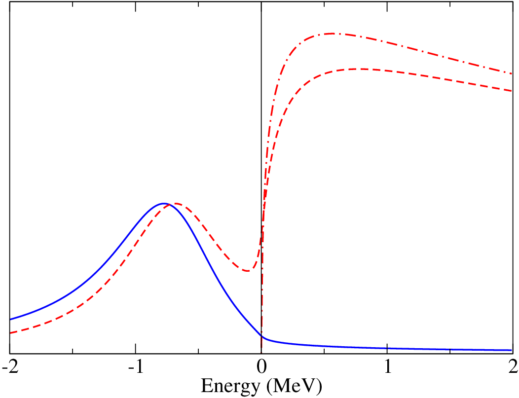
In Figs. 3 and 4, the solid lines are the line shapes in the decay channel for MeV and MeV, respectively. For comparison, the line shapes in the decay channel and the energy distributions are also shown as dashed and dash-dotted lines, respectively. In each figure, the curves are normalized so that the resonances below the threshold have the same maximum values. In both figures, the line shape has a peak below the threshold corresponding to the resonance and a second peak above the threshold corresponding to a threshold enhancement in the production of and . The position and width of the resonance peak is close to that for the line shape. The energy distribution, which vanishes below the threshold, has a peak above the threshold whose width is considerably larger than the width of the resonance. Thus a measurement of the position and width of the peak in the invariant mass distribution should not be interpreted as a measurement of the mass and width of the .
V Analysis of the decay channel


In this section, we analyze recent data from the Belle and Babar Collaborations on the line shape of the in the decay mode [11, 12]. We consider the energy distribution for and in the interval from 0 to 100 MeV. For our two data samples, the total number of and events accumulated and the number of candidate events for the decay of into are as follows:
- •
Babar Collaboration [11]: , 172 events in 50 bins of width 2 MeV,
- •
Belle Collaboration [12]: , 171 events in 50 bins of width 2 MeV.
The data are shown in Figs. 6 and 7. The vertical error bar in a bin with events is . The horizontal error bar indicates the width of the bin.
We take the distribution in the energy to be given by Eqs. (25), (27), and (28). This energy distribution should be accurate within about an MeV of the threshold. We assume that the dominant contributions to the signal come from this threshold region. To predict the number of events in a given bin of invariant mass, we need to take into account the background and the energy resolution of the experiment. The predicted number of events in an energy bin of width centered at can be expressed as
where takes into account the background. Our energy interval 0–100 MeV is narrow enough that the background contribution to the distribution in can be taken as a constant multiplied by , which is the energy dependence of the phase space. The experimental resolution is taken into account through a convolution with a Gaussian resolution function with an energy-dependent width :
| (30) |
We follow Ref. [17] in taking the width for both experiments to be the same energy-dependent function:
| (31) |
This may be too crude a model for the effects of the experimental resolution in this channel, but we will use it for illustrative purposes anyway.
| data set | |||||||
|---|---|---|---|---|---|---|---|
| Babar | 0 | ||||||
| Babar | |||||||
| Belle | 0 | ||||||
| Belle |
We assume that the number of events in each bin of the smeared energy has a Poisson distribution whose mean value is given by in Eq. (). We fix the width at 65.5 keV. The adjustable parameters are , , , and . We determine the best fit to these parameters by maximizing the likelihood for the observed distribution. For both the Belle and Babar data sets, we carry out two fits: one with and one with as a fitting parameter. The results of our four analyses are presented in Table 2. The error bars are determined in the same way as those in Table 1, except that the uncertainty of MeV in the threshold energy does not enter because the experimental energies were measured relative to this threshold.

In the fits to the Babar and Belle data with treated as a fitting parameter, the maximum likelihood is obtained for , which is the smallest possible physical value. This suggests that our model for the experimental resolution in Eq. (31) may provide too much smearing of the energy distribution. The best fit to the Babar data gives a line shape whose peak is below the threshold by about 2.4 MeV, which is incompatible with the assumption MeV that we used to derive analytic expressions for the line shape and the energy distribution. The best fit to the Belle data gives a line shape whose peak is below the threshold by only about 0.05 MeV, which is comparable to the width MeV. The value of from the fit to the Belle data is about an order of magnitude smaller than that from the fit to the Babar data. Since the Belle fit does not satisfy , the value of should not be interpreted literally as the product of branching fractions. It is simply a parameter used to specify the normalization of the line shape in Eq. (22). The Babar fit does satisfy , so the value of can be interpreted as the product of branching fractions. Dividing by the value for from Table 1, we obtain a branching ratio for to of approximately 0.004. This implies that short-distance decay modes account for most of the width of the resonance. However the value for the best fit implies that the contribution to the width from short-distance decay modes is negligible. A possible explanation for this inconsistency is that the simple model for the energy resolution given in Eqs. (30) and (31) is inadequate.
In Fig. 8, we show the line shapes corresponding to the best fit to the Belle data for . The line shape in the decay channel, the line shape in the decay channel, and the energy distribution are shown as solid, dashed, and dash-dotted lines, respectively. The curves are normalized so that the resonances below the threshold have the same peak height. The line shape has a single peak below the threshold whose position and width are close to those for the peak in the line shape. It is this peak that should be identified with the resonance. The energy distribution, which vanishes below the threshold, has a peak above the threshold whose width is considerably larger than that of the resonance. It is also much narrower than the smeared energy distribution shown in Fig. 7.
VI Critique of Previous Analyses
In this section, we discuss how the analysis presented in this paper could be improved. We also point out errors and misconceptions in previous theoretical analyses of the line shapes of the .
The most limiting aspect of our analysis was the use of the analytic expression in Eq. (22) for the line shape in the decay channel. The derivation of this expression involved the assumption MeV. It requires most of the events to be produced with energy within an MeV of the threshold. In particular, it requires the width of the resonance to be much less than an MeV. This limitation can be relaxed by replacing the invariant mass distribution in Eq. (22) by the differential decay distribution in Eq. (13). Given our prescription for in Eq. (22), the normalization of the differential decay rate is determined:
| (32) | |||||
where is given in Eq. (16). The integral over the momenta and must be evaluated numerically.
Another limiting aspect of our analysis was ignoring the effects of the charged charm meson pairs and . They can produce significant interference effects for as small as 1/4 of the 8.1 MeV splitting between the and thresholds [20]. The effects of charged charm meson pairs were first considered by Voloshin [16], but there were conceptual errors in his analysis. A correct analysis was presented by Braaten and Lu [20]. It involves the matrix of S-wave scattering amplitudes between the neutral channel labelled by subscript 0 and the charged channel labelled by subscript 1. The parameters in these scattering amplitudes are the inverse scattering lengths and for charm mesons in the channels with isospin 0 and 1 in the isospin symmetry limit. The coupled-channel expressions for the scattering amplitudes are
| (33a) | |||||
| (33b) | |||||
| (33c) | |||||
where the denominator is
| (34) |
The functions and are
| (35a) | |||||
| (35b) | |||||
where MeV is the reduced mass of and and MeV is the splitting between the and thresholds. In Eq. (35a), is the energy-dependent width of the , which has its physical value 65.5 keV at . In Eq. (35b), is the energy-dependent width of the , which has its physical value 96 keV at MeV and decreases to 1.5 keV at MeV, which is the threshold. Near the threshold, the scattering amplitude in Eq. (33a) reduces to the universal expression in Eq. (2) with
| (36) |
Voloshin’s first conceptual error in Ref. [16] was assuming that a transition that produces the resonance must create the charm mesons in the neutral channel and not in the charged channel. This implies that the amplitudes for the resonant production of an isospin-0 final state such as and an isospin-1 final state such as are proportional to and , respectively. However, since there is resonant scattering between the neutral and charged channels, the resonance can also be produced by a transition that creates the charm mesons in the charged channel. Thus the amplitudes for isospin-0 and isospin-1 final states can also have terms proportional to and , respectively. Voloshin’s second conceptual error was ignoring the constraints of isospin symmetry on the amplitudes for the creation of charm meson pairs by the and transitions. He concluded incorrectly that the rates are proportional to with the same multiplicative constant for and decays. The isospin symmetry constraints derived in Ref. [20] imply that the line shapes are different for and decays and they are determined by three independent multiplicative constants.
Another limiting aspect of our analysis was ignoring the effects of the P-wave charmonium state . This state has the same quantum numbers as the , so it also has an S-wave coupling to charm meson pairs and . Its spin symmetry partner , which was discovered in 2006 by the Belle Collaboration [21], has a mass of about 3930 MeV. Potential models predict the mass of the to be lower by 20 to 50 MeV [22, 23]. Thus its mass could be close enough to the thresholds for the resonant coupling of the to the charm mesons to affect the line shape in this region. Its effects on the line shapes within about an MeV of the threshold would however be negligible. To be more precise, these effects are accurately taken into account through the value of the inverse scattering length . This follows from the universal behavior of an S-wave threshold resonance which makes it insensitive to the mechanism for the resonance. If the mass of the is extremely close to the threshold, it is transformed by its resonant couplings to the charm mesons into a charm meson molecule whose constituents have a large mean separation. Thus far there has been no quantitative analysis of the effects of the on the line shape of the .
In Ref. [15], Hanhart, Kalashnikova, Kudryavtsev, and Nefediev analyzed the line shapes for the using a generalization of a parametrization of the line shape for a near-threshold resonance proposed by Flatté [24]. Their expression for the line shape can be written as , where is the scattering amplitude
| (37) |
is given by Eq. (35a) with , is given by Eq. (35b) with , and is the energy-dependent partial width for short-distance decays of the . This lineshape was also used in a recent analysis by Zhang, Meng and Zheng [17]. Near the threshold, the scattering amplitude in Eq. (33a) reduces to the universal expression in Eq. (2) with and . The coefficient of the term in the denominator of Eq. (37) can be identified as , where is the effective range. In Ref. [15], Hanhart et al. found that the best fits to the Belle and Babar data are in a scaling region of the parameter space in which the term in the denominator is negligible. Thus the only relevant parameters are , , and . The scattering amplitude in Eq. (37) with the term omitted can be obtained from the coupled-channel scattering amplitude in Eq. (33a) by replacing in both the numerator and the last term in the denominator by . Thus the line shape takes into account some of the effects of the coupling between the neutral and charged channels.
One apparent advantage of the line shape that is actually illusory is that it is an integrable function of the energy . The product of branching fractions for a short-distance channel of in the decay can therefore be defined in the conventional way by specifying the energy distribution for the final state to be
| (38) |
This definition of appears to be more natural than the prescription for an threshold S-wave resonance that we introduced in Eq. (8). However the term in Eq. (37) that makes the line shape integrable is the last term . Because the best fit is in a scaling region of the parameter space, varying the parameter while holding the combinations , , and fixed has essentially no effect on the line shape very near the resonance but it does change the interval of the energy that gives significant contributions to the integral of the line shape. The numerical value of is therefore determined by the value of . Thus the definition for in Eq. (37) is in fact an arbitrary prescription specified by the parameter .
In their analysis of the line shape of in the decay mode in Ref. [15], Hanhart et al. made a serious conceptual error. They assumed that the line shape has the form
| (39) |
The factor emphasizes that the line shape was assumed to be zero below the threshold. This reflects the incorrect assumption that events can come only from the production of or above the threshold followed by the decay of or and not from the decay of a bound state below the threshold. However the mass of the is about 7 MeV above the threshold, so there is plenty of phase space for the decay of this bound state into . Moreover the spends most of its time in a configuration in which the charm mesons have large separation, so the or in the bound state can decay almost as if they were free particles. The conceptual error in Ref. [15] was pointed out in Ref. [18], and an analysis that takes into account the decay of the bound state was carried out.
Zhang, Meng and Zheng have recently carried out an updated analysis [17] of the recent data from Babar and Belle using essentially the same line shapes as Hanhart et al. They repeated the conceptual error of Ref. [15] by taking the line shape in to be given by Eq. (39), which does not take into account events produced by decays of the bound state. They determined the location of the poles in the energy for the scattering amplitude in Eq. (37). All of their fits had one pole for which the real and imaginary parts of were less than 1 MeV. This is the pole associated with the S-wave threshold resonance. Their fits also had a second pole on a different Riemann sheet of the complex energy whose absolute value was significantly larger than 1 MeV. This pole is an artifact of the scattering amplitude in Eq. (37) and has no physical significance.
VII Summary
We have carried out an analysis of the line shapes of the in the and decay channels using the most recent data from the Babar and Belle Collaborations. For the signal, we used the line shapes of an S-wave threshold resonance, which differ in several crucial respects from the conventional Breit-Wigner resonance. We took into account the experimental resolution in the energy distributions using Gaussian smearing functions. In the case of the channel, we also took into account the assumption in the experimental analyses that events near the threshold come from and .
The parameters for the S-wave threshold resonance are the real and imaginary parts of the inverse scattering length and a normalization factor that depends on the decay channel . A characteristic feature of an S-wave threshold resonance is that its line shapes are not integrable functions of the energy. One consequence is that the product of the branching fractions for the production of the resonance and its decay into the final state depends on the prescription used to define it. Our prescription for is specified by the analytic expression for the line shape in Eq. (8). Our prescription for is specified by the analytic expression for the line shape in Eq. (32). The parameters for our fits to the Babar and Belle data in the and decay channels are given in Tables 1 and 2.
Because the line shape of an S-wave threshold resonance is not an integrable function of the energy, a prescription is required to define the binding energy and the width of the . Our prescriptions for the binding energy and the width are that the pole in the amplitude as a function of the complex energy are at . Given the values of and , and can be calculated using Eqs. (3). An alternative pair of variables that can in principle be measured directly are the position of the peak in the line shape and its full width at half-maximum . Given the values of and , and can be calculated by solving Eqs. (4) and (5). The values of , , , and for our fits to the Babar and Belle data in the and decay channels are listed in Tables 1 and 2.
We carried out two fits to each of the data sets from the Belle and Babar Collaborations, one with and one with as a fitting parameter. The best fits to the smeared line shapes in the decay channel are shown in Figs. 1 and 2. The best fits to the smeared energy distributions are shown in Figs. 6 and 7. The line shapes in the and decay channels and the energy distributions for three of the best fits are shown in Figs. 3, 4, and 8. The line shape has a peak below the threshold whose position and width are close to those for the line shape. It is this peak that should be identified as the resonance. The energy distribution, which vanishes below the threshold, has a peak above the threshold whose width is considerably larger than the width of the resonance. Thus measurements of the position and width of the peak in the invariant mass distribution should not be interpreted as measurements of the mass and width of the .
In our analyses of the energy distributions measured by the Babar and Belle Collaborations, we took into account the assumption that events near the threshold come from and . Even though the energy distributions vanish below the threshold, our analyses of these distributions gave values for the position of the resonance that were below the threshold. In our analyses with as a fitting parameter, the best fits were for , which is the minimum physical value. In contrast, the best fits to the Babar and Belle data on gave MeV and 12.0 MeV, respectively. The preference for the value in the fit to the data could be an artifact of the simple model for the energy resolution given in Eqs. (30) and (31). Because this model is questionable, we regard our analyses of the data as only illustrative. They are no substitute for analyses by the experimental collaborations that take all the correlated errors properly into account. In a careful analysis, it would be better to use the differential decay distribution in Eq. (32) instead of our analytic expression for the line shape in Eq. (22). Finally an analysis of the decay channel similar to the original Belle analysis in Ref. [10] would be preferable to one in which events near the threshold are interpreted as or . If such an analysis gave resonance parameters for the that are close to those from analyses of the channel, it would go a long way towards solidifying a consensus in the high energy physics community on the nature of the .
Acknowledgements.
This research was supported in part by the Department of Energy under grant DE-FG02-91-ER40690.References
- [1] S.K. Choi et al. [Belle Collaboration], Phys. Rev. Lett. 91, 262001 (2003) [arXiv:hep-ex/0309032].
- [2] B. Aubert et al. [BABAR Collaboration], Phys. Rev. D 77, 111101 (2008) [arXiv:0803.2838 [hep-ex]].
- [3] I. Adachi et al. [Belle Collaboration], arXiv:0809.1224 [hep-ex].
- [4] T. Aaltonen et al. [CDF Collaboration], arXiv:0906.5218 [hep-ex].
- [5] K. Abe et al., arXiv:hep-ex/0505037.
- [6] B. Aubert et al. [BABAR Collaboration], Phys. Rev. D 74, 071101 (2006) [arXiv:hep-ex/0607050].
- [7] B. Fulsom et al. [BABAR Collaboration], arXiv:0809.0042 [hep-ex].
- [8] K. Abe et al., arXiv:hep-ex/0505038.
- [9] A. Abulencia et al. [CDF Collaboration], Phys. Rev. Lett. 98, 132002 (2007) [arXiv:hep-ex/0612053].
- [10] G. Gokhroo et al., Phys. Rev. Lett. 97, 162002 (2006). [arXiv:hep-ex/0606055].
- [11] B. Aubert et al. [BABAR Collaboration], arXiv:0708.1565 [hep-ex].
- [12] I. Adachi et al. [Belle Collaboration], arXiv:0810.0358 [hep-ex].
- [13] E. Braaten and H.W. Hammer, Phys. Rept. 428, 259 (2006). [arXiv:cond-mat/0410417].
- [14] C. Amsler et al. [Particle Data Group], Phys. Lett. B 667, 1 (2008).
- [15] C. Hanhart, Yu.S. Kalashnikova, A.E. Kudryavtsev, and A.V. Nefediev, Phys. Rev. D 76, 034007 (2007) [arXiv:0704.0605 [hep-ph]].
- [16] M.B. Voloshin, Phys. Rev. D 76, 014007 (2007) [arXiv:0704.3029 [hep-ph]].
- [17] O. Zhang, C. Meng and H. Q. Zheng, arXiv:0901.1553 [hep-ph].
- [18] E. Braaten and M. Lu, Phys. Rev. D 76, 094028 (2007) [arXiv:0709.2697 [hep-ph]].
- [19] M. B. Voloshin, Phys. Lett. B 579, 316 (2004) [arXiv:hep-ph/0309307].
- [20] E. Braaten and M. Lu, Phys. Rev. D 77, 014029 (2008) [arXiv:0710.5482 [hep-ph]].
- [21] S. Uehara et al. [Belle Collaboration], Phys. Rev. Lett. 96, 082003 (2006) [arXiv:hep-ex/0512035].
- [22] T. Barnes, S. Godfrey and E. S. Swanson, Phys. Rev. D 72, 054026 (2005) [arXiv:hep-ph/0505002].
- [23] E. J. Eichten, K. Lane and C. Quigg, Phys. Rev. D 73, 014014 (2006) [Erratum-ibid. D 73, 079903 (2006)] [arXiv:hep-ph/0511179].
- [24] S. M. Flatte, Phys. Lett. B 63, 224 (1976).