Scanning the Parameter Space of Holographic Superconductors
Abstract:
We study various physical quantities associated with holographic s-wave superconductors as functions of the scaling dimensions of the dual condensates. A bulk scalar field with negative mass squared , satisfying the Breitenlohner-Freedman stability bound and the unitarity bound, and allowed to vary in unit intervals, were considered. We observe that all the physical quantities investigated are sensitive to the scaling dimensions of the dual condensates. For all the , the characteristic lengths diverge at the critical temperature in agreement with the Ginzburg-Landau theory. The Ginzburg-Landau parameter, obtained from these length scales indicates that the holographic superconductors can be type I or type II depending on the charge and the scaling dimensions of the dual condensates. For a fixed charge, there exists a critical scaling dimension, above which a holographic superconductor is type I, below which it becomes a type II.
Keywords:
Holographic superconductors, AdS/CFT correspondence1 Introduction
The correspondence between gravitational theories in anti-de Sitter spacetime and certain quantum field theories [1] provides a unique way in which to study the strongly coupled sector of many quantum field theories. This remarkable result from string theory has allowed some insight [2] to be gained into why the quark-gluon plasma produced at the relativistic heavy ion collider (RHIC) behaves like an almost perfect fluid [3] (in contrast to the prediction of a high viscosity by perturbative quantum chromodynamics (QCD) [4]). This remarkable result inspired the application of AdS/CFT techniques to certain condensed matter systems. Phenomena such as the Hall effect and the Nernst effect appear to have their dual gravitational descriptions [5, 6, 7].
This technique has been employed recently, to shed some light on strongly coupled systems that undergo superconducting instabilities at a critical temperature (see [8, 9] for a review). It is understood [10, 11] that a quantum field theoretic description of condensed matter systems is possible in the vicinity of the quantum critical point (QCP), where the relevant scale invariant theories are similar to field theories describing second-order phase transitions, for example Ginzburg-Landau theory. As the QCP is approached, systems11 1 For example, spin systems. with the dynamical critical exponent become invariant under re-scalings of time and distance. This scale invariant symmetry forms part of the larger conformal symmetry group [12, 9] of the quantum field theory, where is the number of spatial dimensions. The emergence of this symmetry near the QCP implies that its dual gravitational description must reside in anti-de Sitter spacetime with an additional spatial dimension [8, 13].
According to the model of holographic superconductivity proposed in [14], one can study strongly coupled s-wave superconductors, at a finite temperature and chemical potential, by considering a gravitational theory with an action which has a black hole solution. The black hole, in this case, is charged under a gauge field with a minimally coupled complex scalar field . The no hair theorem does not apply if the scalar field has a non-trivial coupling to the gauge field [15]. In this set up, the symmetry breaking in the bulk theory, which corresponds to a quantum phase transition to the superconducting phase in the boundary theory, is triggered by a position dependent negative mass squared formed from the gauge covariant derivative [16]. Its contribution becomes significant near the horizon of the black hole, thereby forcing the scalar field to condense.
This model has been studied in various limits by several authors. For example, the authors of [17, 18, 19, 20, 21, 22] mapped the phase diagram of the holographic superconductors in the presence of an external magnetic field. They also found and analyzed the physical properties of the vortex and droplets solutions for a scalar field with ( will be defined defined shortly.). The hydrodynamics of holographic superconductors was studied in detail in [23]. The effect of a vector current on the order of the phase transition was explored in [24]. The authors of [25] showed that superconductivity is possible for a scalar field of various masses in and bulk dimensions. A proposal on how to calculate the superconducting characteristic length analytically, in the vicinity of QCP, was suggested in [26]. The effects of gravitational backreaction were considered, and a study made, for , of the type of the holographic superconductors in [27, 28]. So far there has not been any work which discusses the relationship between the physical quantities associated with the model and the scaling dimensions of the dual condensates.
The objective here is to go beyond the extension of the model already discussed in [25] and to include a wider range of values of , satisfying the Brietenlohner-Freedman (BF) stability bound [29] and the unitarity bound. We find it most convenient to choose values of in the interval of units. We shall focus our attention primarily on scalar fields with fall-offs at the AdS boundary, which are normalizable. Based on this behavior at the boundary, the scalar field naturally split into two pieces, and , with slower and faster fall-offs respectively. These describes different condensates with distinct superconducting phases and different scaling dimensions. We shall calculate each physical quantity associated with the condensates at a fixed temperature and for each value of , which will allow us to ascertain the dependence of this physical quantity on the scaling dimension.
This report is organized as follows: In section 2, we define our conventions and derive the equations of motion. In section 3, we show that the superconducting phase of holographic superconductors of the class is very different from that of the class . We present a discussion of the conductivity in section 4 and show that in the limit in which the frequency approaches zero (), the superfluid density can be obtained from the frequency dependent conductivity. In section 5, we solve the equations of motion perturbatively in order to calculate the characteristic lengths and the Ginzburg-Landau parameter. The conclusion is provided in section 6, while various results relating to the conductivity in the boundary theory are presented in the appendices.
2 Background Equations of Motion
The action of a gravitational theory with a black hole solution in anti de Sitter spacetime coupled to a matter field is given by
| (1) |
where is the Einstein-Hilbert action with a negative cosmological constant
| (2) |
with related to Newton’s gravitational constant in dimensions . The cosmological constant depends on the radius of curvature of the anti de Sitter spacetime, , . is the action for the Abelian Higgs system expanded to quadratic order in the scalar field
| (3) |
where the gauge field and the scalar field are coupled through the gauge covariant derivative, . Here is the spacetime covariant derivative, is the gauge field, with associated field strength , and is a complex scalar field. In the probe limit, the matter field can be re-scaled as
| (4) | |||
which ensures that the quadratic potential scales as and the entire matter action as . In the limit , the action for Abelian-Higgs system decouples from the Einstein-Hilbert action . As noted in [14], the probe approximation remains valid as long as and scalar potential are not large in the Planck limit. Another way to implement the probe approximation suggested in [30], is to consider a formal expansion of the full backreacted geometry in inverse powers of . Then the leading order matter solutions will depend on as , while the leading order metric receives corrections.
The equations of motion for the scalar field and Maxwell fields reads
| (5) |
| (6) |
where the current is given by
| (7) |
We consider the planar black hole ansatz
| (8) |
where and runs from to . Here is the event horizon and the Hawking temperature of the black hole is given by
| (9) |
It is more convenient to make a change of coordinates , so that the metric (8) becomes
| (10) |
where and . Here and is the event horizon and AdS boundary respectively. We consider the following ansatze22 2 From these ansatze we can see that the phase of the scalar field is fixed. for the matter fields and . Using the ansatze in the equations of motion, the scalar and gauge fields yield respectively
| (11) |
and
| (12) |
where and . Regularity at the horizon requires
| (13) | |||
Near the boundary the scalar field and the scalar potential behave as
| (14) | |||
where is the dimension of the dual operator, which satisfies the relation
| (15) |
with solutions . The stability of AdS vacuum, requires that the scalar field of negative mass squared must satisfy the BF bound [29], and in general the unitarity bound [31], . In the analysis that follows, we consider the values of within the range . Both modes of the asymptotic values of the scalar fields whose are within this range are normalizable, except at the saturation of the BF bound. For , only the is normalizable, since is below the unitarity bound. As mentioned in the introduction our primary focus is on the scalar fields with within this range , which we can achieve by considering in unit interval. The fixed interval makes the analysis and interpretation of the results less challenging.
The AdS/CFT dictionary [32, 33] relates the constant coefficients of the asymptotic solutions (equation (14)) to physical quantities in the boundary theory. The coefficients are coefficients of the normalizable modes of the scalar field equation, they both correspond to expectation values in the dual field theory . and correspond to the chemical potential and charge density in the dual field theory, respectively.
3 Phase Transitions for Various Condensates
Apart from the trivial solutions and , a non-trivial solution to equations (11) and (12) which describe the superconducting phase in the dual field theory, exist below a critical temperature. The critical temperature is defined, for , when vanishes and for , when vanishes. We present the solutions to equations (11) and (12) obtained numerically in figure 1.


The temperature scales as and in the and boundary theory respectively. Notice that the condensates of the class converge at before they collectively diverge. The signatures of the divergence near zero temperature become more pronounced as approaches the unitarity bound. A similar divergence was observed in [14] for and was attributed to the probe approximation. But recent study [28] which considered gravitational backreaction, also show some signatures of divergence for when the charge becomes large. This divergence might be an artifact of large N. There are obvious differences between the superconducting phase of and that of . The condensates of the class show a gradual transition to the superconducting phase33 3 In bulk dimensions the range of permissible values of is small hence we did not distinguish between the two classes in the graphical representation. All the features as explained for the boundary theory are also present..
The amount of condensate in each case can be calculated from the numerical solutions to equations (11) and (12) at a fixed temperature , in the vicinity of QCP. The results are shown in figure 1 (right).

There appears to be a discontinuity in the amount of condensates between holographic superconductors of the class and that of class at in both and boundary theories. This might be an indication that the two classes have different superconducting coherence factors [14]. The height of the discontinuous gap increases as the temperature decreases.
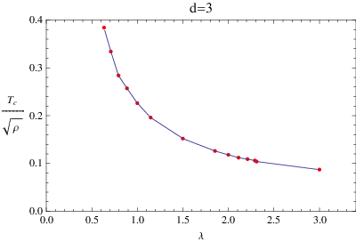
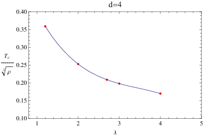
The dependence of the critical temperatures for various condensates on the dimension of the dual operator is shown in figure 3.
.
The condensates with high scaling dimensions have relatively very low critical temperature. In general as the critical temperature decreases as the dimension of dual condensate increases in both the and boundary theories.
4 Conductivity
Within the frame work of the AdS/CFT correspondence, the conductivity in the boundary theory can be calculated from the Maxwell field in the bulk theory. This can be done in the probe limit by perturbing the Maxwell field at zero spatial momentum on the fixed black hole background: With the ansatz for the perturbed Maxwell field, , a linearized equation of motion results
| (16) |
Equation (16) is solved with an ingoing wave boundary condition [34] near the horizon of the black hole in order to suppress near horizon oscillations:
| (17) |
4.1 Conductivity in the ()-dimensional dual field theory
In an odd number of dimensions (e.g. ) the solution to the Maxwell’s equation (16) behaves near the boundary as
| (18) |
From Ohm’s law and the dictionary of AdS/CFT correspondence, the conductivity becomes
| (19) |
The plots of the real and imaginary part of the conductivity against the frequency normalized by individual condensate are shown in appendix A, figure 13 and appendix B, figure 14 for the two classes of holographic superconductors in the boundary theory.
4.2 Conductivity in the ()-dimensional dual field theory
When the bulk dimension is even (e.g. ), there exists a logarithmic divergence of the Maxwell’s field in the action 1:
| (20) |
A boundary counter term may be added to remove the divergence [35], so that the conductivity becomes [25]
| (21) |
The numerical solutions to equation (16) in the boundary theory, is shown in appendix C, figure 15 and for the frequency normalized by the individual superconducting condensate. We could not resolve the delta function at numerically. However, it can be seen from the Kramers-Kronig relation
| (22) |
that there is a delta function at for all the condensates, since is a pole in the imaginary part of the conductivity. The gap frequency remain approximately the same for all the condensates , irrespective of the number of bulk dimensions.
4.3 Superfluid density and magnetic penetration depth
In the limit , the superfluid density is defined as the coefficient of the pole in the imaginary part of conductivity , where is the superfluid density. The results of the superfluid density computed by solving equation (16) in this limit, is shown in figure 4.


The vanishing of at the critical temperature is in agreement with the Ginzburg-Landau theory.
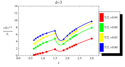
The dependence of the on the scaling dimension calculated at various fixed temperatures below is shown in figure 5.


Observe that for , is not sensitive to changes in , suggesting that this class of holographic superconductors may not be stable against perturbations by external magnetic field, since is related to the current which generate the electromagnetic field if the boundary theory was gauged.
Thus the superfluid density is related to the magnetic penetration depth through the first London equation
| (23) |
where is the charge of the order parameter. Using the Maxwell’s equation for the curl of the magnetic field and assuming that the current at the boundary can generate its own magnetic field44 4 i.e weakly gauging the boundary theory as suggested in [28]., the relation between the superfluid density and the magnetic penetration depth appear more explicitly
| (24) | |||
where . The magnetic penetration depth obtained using this relation for both classes of holographic superconductors is shown in figure 6.


Notice that the magnetic penetration depth diverges at which is an expected behavior. Its dependence on the dimension of the dual operator is presented in figure 7


5 Perturbative Solution
At the quantum critical point, equations (11) and (12) can be solved exactly:
| (25) | |||
Other solutions to equations (11) and (12) can be found in the vicinity of quantum critical point, by a perturbative expansion, since the superconducting condenstate behaves as (see section 3)
| (26) |
and vanishes at . The results of the numerical calculations in section 3 show that at the critical temperature 55 5 We use the conventions of [26]..
Other solutions to equations (11) and (12) may be obtained to higher order in and in the manner which still yield the expected fall offs at the AdS boundary.
| (27) | |||
Using equation (27) in equations (11) and (12) gives
| (28) |
| (29) |
The equations are written in a form most convenient for use in the following analysis. Equation (28) decouples from equation (29) to first order in the perturbative expansion. We make the following definitions for clearer presentation:
| (30) | |||
5.1 Superconducting coherence length
The correlation length of the order parameter is related to the superconducting coherence length , which appears as a complex pole of the static correlation function of the order parameter fluctuation in Fourier space [26]:
| (31) |
Following the technique of AdS/CFT correspondence, this correlation length may be calculated within the probe approximation by perturbing the Maxwell and scalar fields on a fixed black hole background. We consider only the linear perturbation, with fluctuations of the fields in the direction, in the form
| (32) | |||
Using (32) on the perturbed Maxwell and scalar fields give the following eigenvalue equations
| (33) |
| (34) |
| (35) |
where . Regularity at the horizon implies that
| (36) | |||
Analytical treatment is possible for the eigenvalue equations in the limit [26].
| (37) | |||
The solution to equation (37) of interest are those that satisfy the regularity condition at the horizon (36) and have an expected fall off at the AdS boundary (equation 14). One trivial solution is the zeroth order solution and :
| (38) | |||
Non-trivial solutions can be found by a series expansion around the zeroth order solution in powers of
| (39) | |||
Substituting the expansion (39) into equation (37) yields
| (40) |
| (41) |
In this approximation it is easy to see that the equations of motion for and only differ by a factor of two. Equation (40) can be solved for by defining an inner product for the states and which satisfy the boundary condition at the AdS boundary and is well behaved at the horizon (36).
| (42) |
Because is hermitian for non-zero negative mass squared, taking the inner product of equation (40) gives
| (43) |
Using the inner product (42) and the constraint in equation (43) we obtain
| (44) |
Equation (44) may be simplified by considering the equation of motion for the mode :
| (45) |
Since equation (42) is well defined for and it is hermitian, the first term in the right hand side of equation (44) is zero. Using equation (42) and , the eigenvalue in a first order approximation may be written as.
| (46) |
where
| (47) | |||
This result was first derived in [26] for , and it is shown to hold for all the masses that satisfy the unitarity bound in dimensions, except for where the scalar potential diverges. Now the superconducting coherence length is given by
| (48) |
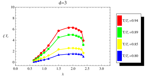
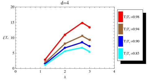
Figure 8 shows the results obtained from calculating the using equation (48) for various condensates. We have used the boundary conditions obtained in section 3 to solve for and .


The numerical accuracy becomes very unsatisfactory for . As a result, we did not include it in the figure 8. The dependence of the superconducting correlation length on the scaling dimensions of the dual condensates is shown in figure 9.
5.2 Magnetic penetration depth
As stated in section 4, the magnetic penetration depth may be calculated from the London current. This can also be calculated by solving equation 35 perturbatively in the limit at zero frequency and momentum. The relevant portion of the Maxwell’s equation is given by
| (49) |
The Maxwell field can be expanded as in the neighborhood of the QCP, which leads to the following equations
| (50) |
| (51) |
where the subscript,, has been dropped for clarity. One of the solutions to equation (50), which satisfies the required boundary conditions is
| (52) |
where is a constant. Hence the first order mode becomes
| (53) |
Integrating this expression (53) yields
| (54) |
Here is the constant of integration. Using
| (55) |
Near the boundary
| (56) |
From the dictionary of AdS/CFT correspondence, the current is identified as
| (57) |
and, for , the current becomes
| (58) |
The magnetic penetration depth is then defined (see equation 24) as
| (59) |
Using equation (48) and (59), the Ginzburg-Landau parameter becomes
| (60) |
To solve for we use the relation to compute instead of . This offers some numerical simplification. The results of the numerical computations are presented in figure 10.


The dependence of the magnetic penetration depth on the scaling dimensions of the dual condensates is shown in figure 11.


Observe that the results of the magnetic penetration depth, calculated using a perturbative approach and the one calculated from superfluid density are in agreement. This agreement show that the perturbative treatment captures the physics of interest in the vicinity of the QCP.
The Ginzburg-Landau parameter can be calculated from equations (48) and (59). The results obtained are plotted in figure 12 against the dimension of the dual condensate.


In Ginzburg-Landau theory, the coefficient classifies superconductors into two types, i.e for type I superconductors and for type II superconductors. If our boundary theory was gauged, the results in figure 12 show that at , there is a change in the relative size of . An obvious interpretation is that for superconducting condensates are of type II, while for they are of type I. It is interesting to see that similar clear distinction also exist for holographic superconductors. Although, we should note that the London current also depends on , which was scaled away in the probe limit. The effect of large but finite is to ensure that is greater than , i.e the condensate must be type II. Despite being large, there are still indications that a holographic superconductor can be type I. This result is in agreement with Maeda et. al. [26], who suggested that holographic superconductors which have low critical temperature are type I. But Hartnoll et. al. [28] showed that holographic superconductor corresponding to dimension one operator, which they studied with high accuracy is a type II. These results are not in any way contradicting, as we have seen that both deductions are correct limits of the larger class of condensates considered here.
6 Conclusion
We have studied the dependence of various physical quantities associated with the holographic model of superconductivity on the scaling dimensions of the dual condensates in the () and ()-dimensional boundary theories. Each of these physical quantities was calculated at a fixed temperature, but for different values of mass squared (varied in 0.5 unit intervals) in and bulk spacetime dimensions. We considered mainly bulk scalar fields which have normalizable fall-offs at the AdS boundary. The results of this indicate that, there are two distinct superconducting condensates dual to the two modes of scalar field, which have different fall-off behaviors at the AdS boundary. The amount of the condensate dual to the bulk scalar field with slower fall-off converges, before diverging collectively near zero temperature. Its superconducting phase is different from that of the scalar fields with a faster fall-off . Certain features indicating a discontinuity in the amount of condensates were observed between condensates of the class and those of the class at . This discontinuity distinguishes between the two classes. The Ginzburg-Landau parameter , obtained from the superconducting coherence length and magnetic penetration depth , indicates that there is a critical scaling dimension at which the holographic superconductors change from type II to type I. Type I holographic superconductors have very low critical temperatures, unlike those of type II, which have relatively high critical temperatures.
It would be very interesting to extend the computations presented in this paper to include the effects of the backreaction of the scalar field on the gravitational background. This would enable us to understand the source of the divergence for the condensates of the class . A treatment involving a complete backreacted geometry would shed some light on the class of condensate that would be associated with the vortex and droplets solutions found in [18, 19]. Based on an understanding of real superconductors, one would not expect a type I holographic superconductor to support a stable vortex solution. One might also repeat the analysis presented here for the action, involving a matter field considered in [36]. This would indicate whether the features observed here are general, and might apply to an entire class of theories with gravity duals.
Acknowledgement
It is a great pleasure to thank Sean Hartnoll and Jeff Murugan for many discussions and special assistance. I benefited from discussions with Julian Sonner, Palleb Basu, Petja Salmi and Matthew Roberts. I thank Alex Hamilton and Andrea Prinsloo for technical assistance on the draft. I acknowledge the financial assistance of NASSP, South Africa, in the form of scholarship, towards this research.
Appendix A Conductivity in ()-dimensional Boundary Theory ()


Appendix B Conductivity in ()-dimensional Boundary Theory ()


Appendix C Conductivity in ()-dimensional Dual Field Theory


References
- [1] J. M. Maldacena, “The large N limit of superconformal field theories and supergravity,” Adv. Theor. Math. Phys. 2 (1998) 231–252, arXiv:hep-th/9711200.
- [2] P. Kovtun, D. T. Son, and A. O. Starinets, “Viscosity in strongly interacting quantum field theories from black hole physics,” Phys. Rev. Lett. 94 (2005) 111601, arXiv:hep-th/0405231.
- [3] M. Luzum and P. Romatschke, “Conformal Relativistic Viscous Hydrodynamics: Applications to RHIC results at ,” Phys. Rev. C78 (2008) 034915, arXiv:0804.4015 [nucl-th].
- [4] G. Baym, H. Monien, C. J. Pethick, and D. G. Ravenhall, “TRANSVERSE INTERACTIONS AND TRANSPORT IN RELATIVISTIC QUARK - GLUON AND ELECTROMAGNETIC PLASMAS,” Phys. Rev. Lett. 64 (1990) 1867–1870.
- [5] S. A. Hartnoll and C. P. Herzog, “Ohm’s Law at strong coupling: S duality and the cyclotron resonance,” Phys. Rev. D76 (2007) 106012, arXiv:0706.3228 [hep-th].
- [6] S. A. Hartnoll, P. K. Kovtun, M. Muller, and S. Sachdev, “Theory of the Nernst effect near quantum phase transitions in condensed matter, and in dyonic black holes,” Phys. Rev. B76 (2007) 144502, arXiv:0706.3215 [cond-mat.str-el].
- [7] S. A. Hartnoll and P. Kovtun, “Hall conductivity from dyonic black holes,” Phys. Rev. D76 (2007) 066001, arXiv:0704.1160 [hep-th].
- [8] S. A. Hartnoll, “Lectures on holographic methods for condensed matter physics,” arXiv:0903.3246 [hep-th].
- [9] C. P. Herzog, “Lectures on Holographic Superfluidity and Superconductivity,” arXiv:0904.1975 [hep-th].
- [10] S. Sachdev, Quantum Phase Transitions. Cambridge University Press, 1999.
- [11] J. A. Hertz, “Quantum critical phenomena,” Phys. Rev. B14 (1976) 1165–1184.
- [12] S. Sachdev, “Exotic phases and quantum phase transitions: model systems and experiments,” arXiv:0901.4103 [cond-mat.str-el].
- [13] S. Sachdev and M. Mueller, “Quantum criticality and black holes,” arXiv:0810.3005 [cond-mat.str-el].
- [14] S. A. Hartnoll, C. P. Herzog, and G. T. Horowitz, “Building a Holographic Superconductor,” Phys. Rev. Lett. 101 (2008) 031601, arXiv:0803.3295 [hep-th].
- [15] S. S. Gubser, “Phase transitions near black hole horizons,” Class. Quant. Grav. 22 (2005) 5121–5144, arXiv:hep-th/0505189.
- [16] S. S. Gubser, “Breaking an Abelian gauge symmetry near a black hole horizon,” Phys. Rev. D78 (2008) 065034, arXiv:0801.2977 [hep-th].
- [17] T. Albash and C. V. Johnson, “A Holographic Superconductor in an External Magnetic Field,” JHEP 09 (2008) 121, arXiv:0804.3466 [hep-th].
- [18] T. Albash and C. V. Johnson, “Phases of Holographic Superconductors in an External Magnetic Field,” arXiv:0906.0519 [hep-th].
- [19] T. Albash and C. V. Johnson, “Vortex and Droplet Engineering in Holographic Superconductors,” arXiv:0906.1795 [hep-th].
- [20] M. Montull, A. Pomarol, and P. J. Silva, “The Holographic Superconductor Vortex,” arXiv:0906.2396 [hep-th].
- [21] E. Nakano and W.-Y. Wen, “Critical magnetic field in a holographic superconductor,” Phys. Rev. D78 (2008) 046004, arXiv:0804.3180 [hep-th].
- [22] W.-Y. Wen, “Inhomogeneous magnetic field in AdS/CFT superconductor,” arXiv:0805.1550 [hep-th].
- [23] I. Amado, M. Kaminski, and K. Landsteiner, “Hydrodynamics of Holographic Superconductors,” JHEP 05 (2009) 021, arXiv:0903.2209 [hep-th].
- [24] A. M. P. Basu and H. H. Shieh, “Supercurrent: Vector hair for an ads black hole,” (2008 [arXiv:0809.4494 [hep-th]]) .
- [25] G. T. Horowitz and M. M. Roberts, “Holographic Superconductors with Various Condensates,” Phys. Rev. D78 (2008) 126008, arXiv:0810.1077 [hep-th].
- [26] K. Maeda and T. Okamura, “Characteristic length of an ads/cft superconductor,” Phys. Rev. D 78 (10600 2008[arXiv:0809.3079[hep-th]]) .
- [27] S. S. Gubser and A. Nellore, “Low-temperature behavior of the Abelian Higgs model in anti-de Sitter space,” JHEP 04 (2009) 008, arXiv:0810.4554 [hep-th].
- [28] S. A. Hartnoll, C. P. Herzog, and G. T. Horowitz, “Holographic Superconductors,” JHEP 12 (2008) 015, arXiv:0810.1563 [hep-th].
- [29] P. Breitenloher and D. Z. Freedman, “Stability in gauge extended supergravity,” 1989 Annals Phys. 144 (1982) .
- [30] A. Yarom, “Fourth sound of holographic superfluids,” arXiv:0903.1353 [hep-th].
- [31] I. R. Klebanov and E. Witten, “AdS/CFT correspondence and symmetry breaking,” Nucl. Phys. B556 (1999) 89–114, arXiv:hep-th/9905104.
- [32] E. Witten, “Anti-de Sitter space and holography,” Adv. Theor. Math. Phys. 2 (1998) 253–291, arXiv:hep-th/9802150.
- [33] S. S. Gubser, I. R. Klebanov, and A. M. Polyakov, “Gauge theory correlators from non-critical string theory,” Phys. Lett. B428 (1998) 105–114, arXiv:hep-th/9802109.
- [34] D. T. Son and A. O. Starinets, “Minkowski-space correlators in AdS/CFT correspondence: Recipe and applications,” JHEP 09 (2002) 042, arXiv:hep-th/0205051.
- [35] M. Taylor, “More on counterterms in the gravitational action and anomalies,” arXiv:hep-th/0002125.
- [36] A. G.-G. S. Franco and D. Rodriguez-Gomez, “A general class of holographic superconductors,” arXiv:0906.1214 [hep-th].