The Evolution of Wide Binary StarsNote: September 16, 2009

Yan-Fei Jiang & Scott Tremaine Affiliation: ¹Department of Astrophysical Sciences, Princeton University, Princeton, NJ 08544, USA Affiliation: ² School of Natural Sciences, Institute for Advanced Study, Einstein Drive, Princeton, NJ 08540, USA

Abstract

We study the orbital evolution of wide binary stars in the solar neighborhood due to gravitational perturbations from passing stars. We include the effects of the Galactic tidal field and continue to follow the stars after they become unbound. For a wide variety of initial semi-major axes and formation times, we find that the number density (stars per unit logarithmic interval in projected separation) exhibits a minimum at a few times the Jacobi radius $r_{J}$ , which equals $1.7\,\mbox{pc}$ for a binary of solar-mass stars. The density peak interior to this minimum arises from the primordial distribution of bound binaries, and the exterior density, which peaks at $\sim 100$ – $300\,\mbox{pc}$ separation, arises from formerly bound binaries that are slowly drifting apart. The exterior peak gives rise to a significant long-range correlation in the positions and velocities of disk stars that should be detectable in large astrometric surveys such as GAIA that can measure accurate three-dimensional distances and velocities.

Keywords:

binaries: general — Galaxy: kinematics and dynamics — solar neighborhood — stars: kinematics

I Introduction

Wide binary stars are disrupted by gravitational encounters with passing stars, molecular clouds, and other perturbers. This process was first investigated by [28], who estimated the $e$ -folding time for disruption of binaries composed of solar-mass stars, with apocenter distances of $1\,\mbox{pc}$ , to be $10\,\mbox{Gyr}$ or less. Other early estimates of the disruption rate are due to [1], [8], [40], [14], [20], [15], [32], and [3]. In the last of these a binary of age $t_{0}$ and component masses $M_{1}$ and $M_{2}$ was estimated to have a 50% survival probability at semi-major axis

a_{1/2}(t_{0})=0.002\frac{(M_{1}+M_{2})\sigma}{G\rho_{2}t_{0}}=3.1\times 10^{4}\,\mbox{AU}\,\frac{M_{1}+M_{2}}{2M_{\odot}}\frac{\sigma}{50\,\mbox{km s}^{-1}}\frac{0.03M_{\odot}^{2}\,\mbox{pc}^{-3}}{\rho_{2}}\frac{10\,\mbox{Gyr}}{t_{0}}.

(1)

Here $3\sigma^{2}$ is the mean-square relative velocity between the center of mass of the binary and the perturbing stars, and $\rho_{2}\equiv\int n(M_{p})M_{p}^{2}dM_{p}$ is the second moment over mass of the number density of stars in the solar neighborhood (cf. eq. 47). This estimate is substantially shorter than Öpik’s, mostly because it includes the cumulative effects of distant, weak encounters (which Öpik recognized to be important but did not compute).

A closely related problem is to estimate the distribution of semi-major axes of wide binaries. For relatively small semi-major axes $a\lesssim a_{1/2}(t_{0})$ the distribution is presumably primordial, and thus reflects the (poorly understood) formation process of wide binaries. At larger semi-major axes $a\gtrsim a_{1/2}(t_{0})$ the distribution ought to be primarily determined by the disruption process. The Fokker–Planck equation that describes the evolution of the semi-major axis distribution (eq. 35) was derived and solved by [20], [32] and [39], who showed that $dn\propto da/a^{2}$ for $a\gtrsim a_{1/2}(t_{0})$ .

Observationally, the distribution of wide binary semi-major axes is determined by measuring the projected separations of common-proper-motion binaries (e.g., Chanamé & Gould 6, Poveda et al. 30, Lépine & Bongiorno 24, Sesar et al. 34; see also Chanamé 7 and references therein). For $a\lesssim 3\times 10^{3}\,\mbox{AU}$ the distribution of separations or semi-major axes¹¹ 1 For a population of binaries at a given semi-major axis $a$ , with other orbital elements assigned as described at the start of §III, the median projected separation is $0.978a$ . Thus we may assume that the distributions of semi-major axes and separations are nearly the same. of disk binaries is approximated well by Öpik’s (1924) law,

dn\propto d\log a=\frac{da}{a}.

(2)

At larger semi-major axes, the number of binaries falls more steeply, roughly as $dn\propto da/a^{1.6}$ for $3\times 10^{3}\,\mbox{AU}\lesssim a\lesssim 10^{5}\,\mbox{AU}$ [24]. The further steepening to $dn\propto da/a^{2}$ that is expected for $a\gtrsim a_{1/2}(10\,\mbox{Gyr})\simeq 3\times 10^{4}\,\mbox{AU}$ is much more difficult to detect. There have been a number of claimed detections of this steepening—often, less accurately, called a “cutoff”—but these are controversial [2, 37, 23, 38, 29, 41, 31]. Measurements of the semi-major axis distribution are likely to improve dramatically in the next few years because of large, accurate proper-motion surveys. In particular, the GAIA spacecraft will determine both proper motions and trigonometric parallaxes for millions of nearby stars with unprecedented accuracy, allowing a far better determination of the binary population at large separations than the ground-based proper motions and photometric parallaxes that have been used in all studies so far.

Large, well-characterized samples of wide binaries have many applications [7]. In particular, the distribution of wide binary semi-major axes can be used to constrain the properties of molecular clouds and other massive structures in the disk, and possible compact objects (MACHOs) in the dark halo [3, 41]. If the distribution of binaries can be measured at separations as large as a few parsecs we expect to see “tidal tails” of the kind that have been detected around globular clusters [26, 4, 13]; the evolution of these structures offers a prototype for the evolution of the phase-space structures in the solar neighborhood caused by the disruption of stellar clusters [10].

Almost all theoretical studies of the expected distribution of wide binaries have made two related approximations that compromise their validity at the largest semi-major axes:

•

The stars are assumed to disappear instantaneously as soon as their orbits become unbound. This is unrealistic because the disruption rate is dominated by weak, distant encounters, so most escaping stars have very small relative velocity and only drift slowly apart.
•

The Galactic tidal field is ignored. The tidal field becomes stronger than the gravitational attraction between the stars in the binary when the separation is roughly the Jacobi or tidal radius, which equals $1.7\,\mbox{pc}=3.5\times 10^{5}\,\mbox{AU}$ for solar-mass stars in the solar neighborhood (eq. 43). Thus the tidal field is already significant at the separations ( $\sim 10^{5}\,\mbox{AU}$ ) probed by current measurements of the wide binary distribution, and dominates the dynamics at larger separations.

Including these two effects is necessary if we are to understand the expected distribution of binary stars—bound and unbound—at semi-major axes of $10^{4}\,\mbox{AU}$ and larger. To achieve this understanding is the primary goal of this paper. We restrict ourselves to the evolution of disk binaries under the influence of passing stars, although it is straightforward to extend our methods to include either halo binaries or other perturbers such as molecular clouds or massive black holes.

The structure of this paper is as follows. In §II, we describe the basic equations of motion for binary stars in the Galactic tidal field and how we calculate the perturbations from other stars that drive the orbital evolution. We also review the standard analytic treatment of the evolution of bound binaries using a diffusion equation. Then in §III we describe the results from our simulations. Finally, §IV contains a discussion and conclusions, and Appendix A derives an analytic model that approximately describes the diffusion of unbound binary stars.

II Basic equations in the numerical simulation

In this section, we describe the details of our numerical simulation. First, we give the equations of motion of the binary star in Hill’s approximation. Then, we describe how we include the effects of kicks from other stars. Finally, we describe the diffusion approximation, which should be valid for binaries with small semi-major axes.

II.1 Evolution without kicks

We use Hill’s approximation [16, 5, e.g.,] to describe the motion of the binary star in the Galaxy. Hill’s approximation is valid because the mass of the binary is much less than the mass of the Galaxy (by a factor $\sim 10^{11}$ ). Let the masses of the two stars in the binary be $M_{1}$ and $M_{2}$ . We assume that the potential of the Galaxy is symmetric about the plane $Z=0$ , where $(X,Y,Z)$ or $(R,\phi,z)$ is an inertial Cartesian or cylindrical coordinate system with origin at the center of the Galaxy. We introduce a second coordinate system $(x,y,z)$ with origin in the $Z=0$ plane at distance $R_{g}$ from the Galactic center. The $x$ - $y$ and $X$ - $Y$ planes coincide but the origin of the $(x,y,z)$ coordinate system co-rotates with the Galaxy. The $x$ -axis points radially outward, the $y$ -axis points in the direction of Galactic rotation, and the $z$ -axis is perpendicular to the Galactic plane. The $x$ , $y$ and $z$ axes form a right-hand coordinate system. With these conventions, the positive $z$ -axis points toward the South Galactic Pole. The angular speed of the Galaxy at radius $R_{g}$ , which equals the angular speed of the $(x,y,z)$ frame, is $\mathbf{\Omega}_{g}=\Omega_{g}\mathbf{e}_{z}$ in the $z$ or “vertical” direction. The angular speed $\Omega_{g}$ is related to the potential of the Galaxy $\Phi_{0}(R,z)$ by

\Omega_{g}^{2}=\frac{\Phi_{0}^{{}^{\prime}}(R_{g},0)}{R_{g}},

(3)

where $\Phi_{0}^{{}^{\prime}}(R_{g},0)\equiv\partial\Phi_{0}/\partial R|_{(R_{g},0)}$ . As we want to study binary stars in the solar neighborhood, we can just choose $R_{g}$ to be the distance of the Sun from the Galactic center, $R_{g}=8\,\mbox{kpc}$ .

In the co-rotating frame with origin at $R_{g}$ , the position of star $i$ , $i=1,2$ , is labeled by $\mathbf{r}_{i}=(x_{i},y_{i},z_{i})$ . Then in the co-rotating frame with origin at the center of the Galaxy, the star’s position is $\mathbf{R}_{g}+\mathbf{r}_{i}$ , where $\mathbf{R}_{g}=(R_{g},0,0)$ and the equation of motion for either star in the binary system is

\frac{d^{2}(\mathbf{r}_{i}+\mathbf{R}_{g})}{dt^{2}}=-{\mbox{\boldmath$\nabla$}}_{i}\Phi-2\mathbf{\Omega}_{g}\times\frac{d(\mathbf{r}_{i}+\mathbf{R}_{g})}{dt}-\mathbf{\Omega}_{g}\times\left[\mathbf{\Omega}_{g}\times(\mathbf{r}_{i}+\mathbf{R}_{g})\right]\ ,

(4)

where ${\mbox{\boldmath$\nabla$}}_{i}$ is the gradient with respect to $\mathbf{r}_{i}$ . The potential $\Phi$ includes the contribution from the Galaxy $\Phi_{0}$ as well as the potential of the binary stars $\Phi_{b}$ . For $\Phi_{0}$ , we use the distant-tide approximation, which means $\Phi_{0}(R_{g}+x,y,z)$ at the position of a star is expanded with respect to $\Phi_{g}(R_{g},0,z)$ . Then we have

({\mbox{\boldmath$\nabla$}}\Phi_{0})_{\alpha}=\Phi_{0,\alpha}+\sum_{\beta=x,y,z}\Phi_{0,\alpha\beta}\ \beta+O(r^{2}),\quad\alpha=(x,y).

(5)

Here $\Phi_{0,\alpha}\equiv(\partial\Phi_{0}/\partial\alpha)_{(R_{g},0)}$ and $\Phi_{0,\alpha\beta}\equiv(\partial^{2}\Phi_{0}/\partial\alpha\,\partial\beta)_{(R_{g},0)}$ . Equation (4) is correct for any value of $\mathbf{r}_{i}$ ; in particular, when $\mathbf{r}_{i}=0$ , it is correct for the center $\mathbf{R}_{g}$ , and we may subtract the equation for the center from (4) to obtain

$\displaystyle\frac{d^{2}x}{dt^{2}}=$	$\displaystyle-\frac{\partial\Phi_{b}}{\partial x}-\sum_{\beta=x,y,z}\Phi_{0,x\beta}\,\beta-\left[2\mathbf{\Omega}_{g}\times\frac{d\mathbf{r}}{dt}\right]_{x}-\left[\mathbf{\Omega}_{g}\times\left(\mathbf{\Omega}_{g}\times\mathbf{r}\right)\right]_{x},$
$\displaystyle\frac{d^{2}y}{dt^{2}}=$	$\displaystyle-\frac{\partial\Phi_{b}}{\partial y}-\sum_{\beta=x,y,z}\Phi_{0,y\beta}\,\beta-\left[2\mathbf{\Omega}_{g}\times\frac{d\mathbf{r}}{dt}\right]_{y}-\left[\mathbf{\Omega}_{g}\times\left(\mathbf{\Omega}_{g}\times\mathbf{r}\right)\right]_{y},$
$\displaystyle\frac{d^{2}z}{dt^{2}}=$	$\displaystyle-\frac{\partial\Phi_{b}}{\partial z}-\frac{\partial\Phi_{0}}{\partial z}-\left[2\mathbf{\Omega}_{g}\times\frac{d\mathbf{r}}{dt}\right]_{z}-\left[\mathbf{\Omega}_{g}\times\left(\mathbf{\Omega}_{g}\times\mathbf{r}\right)\right]_{z}.$	(6)

We have

\Phi_{0,xx}=\Big(\frac{\partial^{2}\Phi_{0}}{\partial R^{2}}\Big)_{(R_{g},0)},\quad\Phi_{0,yy}=\Big(\frac{1}{R}\frac{\partial\Phi_{0}}{\partial R}\Big)_{(R_{g},0)},\quad\Phi_{0,xy}=0.

(7)

The potential $\Phi_{b}$ for star $i=1,2$ is just the potential from the other star in the binary. Then we have

\Phi_{b1}=-\frac{GM_{2}}{\sqrt{(x_{1}-x_{2})^{2}+(y_{1}-y_{2})^{2}+(z_{1}-z_{2})^{2}}},

(8)

where $(x_{i},y_{i},z_{i})$ denotes the position of star $i$ , and the formula for $\Phi_{b2}$ is obtained by interchanging 1 and 2 in all subscripts. Then the equations of motion for either star are

$\displaystyle\ddot{x_{i}}=$	$\displaystyle 2\Omega_{g}\dot{y_{i}}+\Big[\Omega_{g}^{2}-\Phi_{0}^{{}^{\prime\prime}}(R_{g},0)\Big]x_{i}-\frac{\partial\Phi_{bi}}{\partial x_{i}}\ ,$
$\displaystyle\ddot{y_{i}}=$	$\displaystyle-2\Omega_{g}\dot{x_{i}}+\Big[\Omega_{g}^{2}-\frac{\Phi_{0}^{{}^{\prime}}(R_{g},0)}{R_{g}}\Big]y_{i}-\frac{\partial\Phi_{bi}}{\partial y_{i}}\ ,$
$\displaystyle\ddot{z_{i}}=$	$\displaystyle-\frac{\partial\Phi_{0}}{\partial z_{i}}-\frac{\partial\Phi_{bi}}{\partial z_{i}}\ .$	(9)

As the angular speed $\Omega_{g}$ is related to the potential $\Phi_{0}$ via equation (3), we have

\Phi_{0}^{{}^{\prime\prime}}(R_{g},0)=\Omega_{g}^{2}+2R_{g}\Omega_{g}\frac{d\Omega}{dR}\bigg|_{R_{g}}.

(10)

As usual, the Oort constant $A(R)$ is defined as

A(R)=-\frac{1}{2}R\frac{d\Omega}{dR}\ .

(11)

We label $A_{g}=A(R_{g})$ . Then equation (9) can be simplified to

$\displaystyle\ddot{x_{i}}-2\Omega_{g}\dot{y_{i}}-4\Omega_{g}A_{g}x_{i}=$	$\displaystyle-\frac{\partial\Phi_{bi}}{\partial x_{i}}\ ,$
$\displaystyle\ddot{y_{i}}+2\Omega_{g}\dot{x_{i}}=$	$\displaystyle-\frac{\partial\Phi_{bi}}{\partial y_{i}}\ ,$
$\displaystyle\ddot{z_{i}}+\frac{\partial\Phi_{0}}{\partial z_{i}}=$	$\displaystyle-\frac{\partial\Phi_{bi}}{\partial z_{i}}\ .$	(12)

From equation (8), we have the following relations

M_{1}\frac{\partial\Phi_{b1}}{\partial x_{1}}=-M_{2}\frac{\partial\Phi_{b2}}{\partial x_{2}},\quad M_{1}\frac{\partial\Phi_{b1}}{\partial y_{1}}=-M_{2}\frac{\partial\Phi_{b2}}{\partial y_{2}},\quad M_{1}\frac{\partial\Phi_{b1}}{\partial z_{1}}=-M_{2}\frac{\partial\Phi_{b2}}{\partial z_{2}}.

(13)

The center of mass of the binary system $\mathbf{r}_{\rm{cm}}$ is defined to be

\mathbf{r}_{\rm{cm}}=\frac{M_{1}\mathbf{r}_{1}+M_{2}\mathbf{r}_{2}}{M_{1}+M_{2}}.

(14)

The relative coordinates of the two stars are $\mathbf{r}=\mathbf{r}_{1}-\mathbf{r}_{2}.$ By adding equations (12) multiplied by appropriate coefficients for star $i=1$ and $i=2$ , we get the equation for the motion of the center of mass²² 2 We assume the separation of the two stars along the $z$ direction is much smaller than the thickness of the Galaxy.

$\displaystyle\ddot{x}_{\rm{cm}}-2\Omega_{g}\dot{y}_{\rm{cm}}-4\Omega_{g}A_{g}x_{\rm{cm}}=$	$\displaystyle 0\ ,$
$\displaystyle\ddot{y}_{\rm{cm}}+2\Omega_{g}\dot{x}_{\rm{cm}}=$	$\displaystyle 0\ ,$
$\displaystyle\ddot{z}_{\rm{cm}}+\frac{\partial\Phi_{0}}{\partial z_{\rm{cm}}}=$	$\displaystyle 0\ .$	(15)

Due to the symmetry of the Galactic potential, $(\partial\Phi_{0}/\partial z)_{z=0}=0$ , so for stars not very far from the mid-plane of the Galaxy, we approximately have $\partial\Phi_{0}/\partial z=(\partial^{2}\Phi_{0}/\partial z^{2})_{z=0}\,z$ and we define

\nu_{g}^{2}=\frac{\partial^{2}\Phi_{0}}{\partial z^{2}}\bigg|_{(R_{g},0)},

(16)

where $\nu_{g}$ is the frequency for small oscillations in $z$ . The general solution to the above equations of motion for the center of mass is just epicycle motion,

$\displaystyle x_{\rm{cm}}(t)=$	$\displaystyle x_{g,\rm cm}+X\cos(\kappa_{g}t+\alpha)\ ,$
$\displaystyle y_{\rm{cm}}(t)=$	$\displaystyle y_{g,\rm cm}(t)-Y\sin(\kappa_{g}t+\alpha),\quad y_{g,\rm cm}(t)=y_{g,0}-2A_{g}x_{g,\rm cm}t,\quad Y=\frac{2\Omega_{g}}{\kappa_{g}}X,$
$\displaystyle z_{\rm{cm}}(t)=$	$\displaystyle Z\cos(\nu_{g}t+\alpha_{z}).$	(17)

Here $x_{g,\rm cm}$ , $X$ , $y_{g,0}$ , $Z$ , $\alpha$ , $\alpha_{z}$ are arbitrary constants, and $\kappa_{g}$ is the epicycle frequency defined by

\kappa_{g}^{2}=4\Omega_{g}(\Omega_{g}-A_{g})\ .

(18)

The variables $x_{g,\rm cm}(t)$ and $y_{g,\rm cm}(t)$ give the position of the guiding center—the center of the epicyclic motion—for the center of mass. Subtract equations (12) with $i=2$ from $i=1$ and we get the equations for the relative motion of the two stars

$\displaystyle\ddot{x}-2\Omega_{g}\dot{y}-4\Omega_{g}A_{g}x=$	$\displaystyle-\frac{G(M_{1}+M_{2})x}{(x^{2}+y^{2}+z^{2})^{3/2}}\ ,$
$\displaystyle\ddot{y}+2\Omega_{g}\dot{x}=$	$\displaystyle-\frac{G(M_{1}+M_{2})y}{(x^{2}+y^{2}+z^{2})^{3/2}}\ ,$
$\displaystyle\ddot{z}+\nu_{g}^{2}z=$	$\displaystyle-\frac{G(M_{1}+M_{2})z}{(x^{2}+y^{2}+z^{2})^{3/2}}\ .$	(19)

In this set of equations, the terms involving $\dot{y}$ or $\dot{x}$ arise from the Coriolis force, as we are working in a rotating frame; the terms involving $A_{g}$ or $\nu_{g}$ represent the effect of the Galactic tide, and the terms on the right side represent the gravitational force between the members of the binary system.

Equations (19) show that the relative motion is the same as that of a test particle around an object with the mass $M_{1}+M_{2}$ in the Galactic tidal field. A special solution to the above equations is the stationary solution ( $\ddot{x}=\dot{x}=\ddot{y}=\dot{y}=\ddot{z}=\dot{z}=0$ )

y=z=0,\ x=\pm r_{J},\quad\hbox{where}\quad r_{J}\equiv\left[\frac{G(M_{1}+M_{2})}{4\Omega_{g}A_{g}}\right]^{1/3}\

(20)

is the Jacobi or tidal radius of the binary system. The stationary points are actually the Lagrange points in the three-body system composed of binary star and the Galaxy. As will be seen from our simulations below, the Jacobi radius sets the characteristic scale for the distribution of binary stars at large radii.

Equations (19) admit one integral of motion, the Jacobi constant

	$\displaystyle E_{J}\equiv$	$\displaystyle\frac{1}{2}(\dot{x}^{2}+\dot{y}^{2}+\dot{z}^{2}-4\Omega_{g}A_{g}x^{2}+\nu_{g}^{2}z^{2})-\frac{G(M_{1}+M_{2})}{\sqrt{x^{2}+y^{2}+z^{2}}}$
	$\displaystyle=$	$\displaystyle\frac{1}{2}(\dot{x}^{2}+\dot{y}^{2}+\dot{z}^{2})+\Phi_{\rm{eff}}(x,y,z),$		(21)

where $\Phi_{\rm{eff}}(x,y,z)\equiv\nu_{g}^{2}z^{2}/2-2\Omega_{g}A_{g}x^{2}-G(M_{1}+M_{2})/\sqrt{x^{2}+y^{2}+z^{2}}$ is the effective potential. The Jacobi constant for the stationary solution (20) is called the critical Jacobi constant $E_{c}$ , and is given by

E_{c}=\Phi_{\rm{eff}}(\pm r_{J},0,0)=-2\Omega_{g}A_{g}r_{J}^{2}-\frac{G(M_{1}+M_{2})}{r_{J}}=-\frac{3}{2^{1/3}}(\Omega_{g}A_{g})^{1/3}[G(M_{1}+M_{2})]^{2/3}.

(22)

As $\dot{x}^{2},\dot{y}^{2},\dot{z}^{2}\geq 0$ , the motion is constrained to the region in which $\Phi_{\rm eff}(x,y,z)\leq E_{J}$ , and the boundary of this region is the zero-velocity surface for a given Jacobi constant, defined implicitly by

\Phi_{\rm{eff}}(x,y,z)=E_{J}.

(23)

Refer to caption — Figure 1: Zero-velocity contours in the plane parallel to the Galactic disk, as given by equation (26). The red line is the critical contour on which the effective potential $\Phi_{\rm{eff}}=E_{c}$ . In regions A, B and C, $\Phi_{\rm{eff}}<E_{c}$ and in regions D and E, $\Phi_{\rm{eff}}>E_{c}$ . Binary stars with large separations can either have $\Phi_{\rm{eff}}<E_{c}$ or $\Phi_{\rm{eff}}>E_{c}$ , depending on their positions on this plot. We define bound binaries as those in region A with $E_{J}<E_{c}$ and call all others escaped binaries.

We choose the time unit to be $1/\Omega_{g}$ and the length unit to be $r_{J}$ . Then we can define the following dimensionless variables (see eq. 44 for numerical values of the scaling factors)

\tilde{\mathbf{r}}=\frac{\mathbf{r}}{r_{J}},\quad\tilde{\mathbf{r}}^{\prime}=\frac{\dot{\mathbf{r}}}{\Omega_{g}r_{J}},\quad\tilde{\mathbf{r}}^{\prime\prime}=\frac{\ddot{\mathbf{r}}}{\Omega_{g}^{2}r_{J}}.

(24)

Then equations (19) can be simplified to the following dimensionless form

$\displaystyle\tilde{x}^{\prime\prime}-2\tilde{y}^{\prime}-\frac{4A_{g}}{\Omega_{g}}\tilde{x}=$	$\displaystyle-\frac{4A_{g}}{\Omega_{g}}\frac{\tilde{x}}{(\tilde{x}^{2}+\tilde{y}^{2}+\tilde{z}^{2})^{3/2}}\ ,$
$\displaystyle\tilde{y}^{\prime\prime}+2\tilde{x}^{\prime}=$	$\displaystyle-\frac{4A_{g}}{\Omega_{g}}\frac{\tilde{y}}{(\tilde{x}^{2}+\tilde{y}^{2}+\tilde{z}^{2})^{3/2}}\ ,$
$\displaystyle\tilde{z}^{\prime\prime}+\frac{\nu_{g}^{2}}{\Omega_{g}^{2}}\tilde{z}=$	$\displaystyle-\frac{4A_{g}}{\Omega_{g}}\frac{\tilde{z}}{(\tilde{x}^{2}+\tilde{y}^{2}+\tilde{z}^{2})^{3/2}}\ .$	(25)

Note that the dimensionless equations do not depend on the specific values of the masses $M_{1}$ and $M_{2}$ . Thus the result applies to binaries of any masses. The dimensionless form of the zero-velocity surface projected to the $x$ - $y$ plane is

\tilde{x}^{2}+\frac{2}{\sqrt{\tilde{x}^{2}+\tilde{y}^{2}}}=-\frac{E_{J}}{2r_{J}^{2}A_{g}\Omega_{g}}.

(26)

The zero-velocity contours are shown in Figure 1. Binaries with $E_{J}<E_{c}$ in region A have bounded motion in that they can never escape from A; we call these bound binaries. All others are called escaped binaries.

Once we know the velocity of the center of mass $\dot{\mathbf{r}}_{\rm{cm}}$ and relative velocity $\dot{\mathbf{r}}$ , we can calculate the velocity of each star in the rotating frame from the relations

\dot{\mathbf{r}}_{1}=\dot{\mathbf{r}}_{\rm{cm}}+\frac{M_{2}}{M_{1}+M_{2}}\dot{\mathbf{r}},\quad\dot{\mathbf{r}}_{2}=\dot{\mathbf{r}}_{\rm{cm}}-\frac{M_{1}}{M_{1}+M_{2}}\dot{\mathbf{r}}.

(27)

II.2 Kicks from other stars

In order to study the evolution of the binary systems, we must include the effect of encounters with passing stars and other perturbers (e.g., molecular clouds). In this paper we only discuss the effects of encounters with stars, but we return briefly to the effects of molecular clouds in the discussion of §IV.

As the velocity dispersion of the perturbers ( $\sim 30\,\mbox{km s}^{-1}$ ) is much larger than the velocity difference of the two stars in the binary system ( $\lesssim 1\,\mbox{km s}^{-1}$ ), we can use the impulse approximation, i.e., the encounter with the perturber provides an impulsive kick that changes only the velocity, not the position, of the subject star. For computational efficiency, we do not follow individual encounters but instead consider the total effect of the encounters on the binary system after some time interval $\Delta t_{p}$ , which is generally large enough to include many encounters (see §III.1 for further discussion of this approximation). Let the change of velocity of the subject star after this time interval be $\Delta\mathbf{v}$ . According to the central limit theorem, the effect of a large number of kicks will be the same as that of a Gaussian distribution with the same mean $\boldsymbol{\mu}=\langle\Delta\mathbf{v}\rangle$ and covariance matrix $C_{\alpha\beta}=\langle\Delta v_{\alpha}\Delta v_{\beta}\rangle$ , where the subscripts $\alpha,\ \beta$ refer to the $x$ , $y$ , $z$ directions. The values of $\mu_{\alpha}$ and $C_{\alpha\beta}$ after the time interval $\Delta t_{p}$ can be computed from the diffusion coefficients

\mu_{\alpha}=D[\Delta v_{\alpha}]\Delta t_{p},\quad C_{\alpha\beta}=D[\Delta v_{\alpha}\Delta v_{\beta}]\Delta t_{p}\ .

(28)

We assume that the number density of perturbers with mass in the range $M_{p}\rightarrow M_{p}+dM_{p}$ is $n(M_{p})dM_{p}$ , and that the velocity distribution of the perturbers relative to the center of mass of the binary is isotropic and Maxwellian,

dn=f(v_{p})dM_{p}d\mathbf{v}_{p}=\frac{n(M_{p})}{(2\pi\sigma^{2})^{3/2}}e^{-v_{p}^{2}/(2\sigma^{2})}dM_{p}d\mathbf{v}_{p},

(29)

where $\sigma$ is the relative velocity dispersion. Expressions for the diffusion coefficients are given in equations (7.89) and (7.92) of [5]. The actual relative velocity distribution is more complicated, both because the distribution of stellar velocities in the solar neighborhood is triaxial and because the center of mass of the subject binary star has its own epicyclic motion, but we do not believe that these complications will alter our results significantly. If the velocity of subject star $i$ relative to the center of mass of the binary is $\mathbf{v}_{i}$ , then

	$\displaystyle D[\Delta v_{i,\alpha}]=$	$\displaystyle\frac{v_{i,\alpha}}{v_{i}}D[\Delta v_{\|\|}]_{i},\$
	$\displaystyle D[\Delta v_{i,\alpha}\Delta v_{i,\beta}]=$	$\displaystyle\frac{v_{i,\alpha}v_{i,\beta}}{v_{i}^{2}}\big\{D[(\Delta v_{\|\|})^{2}]_{i}-\frac{1}{2}D[(\Delta v_{\perp})^{2}]_{i}\big\}+\frac{1}{2}\delta_{\alpha,\beta}D[(\Delta v_{\perp})^{2}]_{i},$		(30)

where $D[\Delta v_{||}]$ is the mean change of velocity per unit time along the velocity vector direction $\hat{\mathbf{v}}$ , while $D[(\Delta v_{\perp})^{2}]$ and $D[(\Delta v_{\parallel})^{2}]$ are the mean-square changes per unit time in the velocity perpendicular and parallel to $\hat{\mathbf{v}}$ .

In the limit $|\mathbf{v}_{i}|\ll\sigma$ , we have

$\displaystyle D[\Delta v_{\|\|}]_{i}=$	$\displaystyle\frac{4\sqrt{2\pi}G^{2}(M_{i}\rho_{1}+\rho_{2})\ln\wedge}{3\sigma^{3}}v_{i},\$
$\displaystyle D[(\Delta v_{\|\|})^{2}]_{i}=$	$\displaystyle\frac{8\sqrt{2\pi}G^{2}\rho_{2}\ln\wedge}{3\sigma}\ ,$
$\displaystyle D[(\Delta v_{\perp})^{2}]_{i}=$	$\displaystyle\frac{16\sqrt{2\pi}G^{2}\rho_{2}\ln\wedge}{3\sigma},$	(31)

where

\rho_{k}=\int n(M_{p})M_{p}^{k}\,dM_{p}.

(32)

Here $\wedge$ is defined to be

\wedge=\frac{b_{\rm{max}}v_{\rm{typ}}^{2}}{G(M_{i}+\tilde{M}_{p})},

(33)

where $b_{\rm{max}}$ is the maximum impact parameter considered, $v_{\rm{typ}}$ is the typical relative velocity and $\tilde{M}_{p}$ is the typical perturber mass. Since these parameters enter only logarithmically, we can just assume $\tilde{M}_{p}=M_{\odot}$ and $v_{\rm{typ}}\simeq\sigma$ for simplicity, and the maximum impact parameter $b_{\rm{max}}$ can be chosen to be the half of the separation of the two stars when we apply the kick³³ 3 We have checked that even though the separations of binary stars have a wide range, different choices of $b_{\rm{max}}$ will not change the results significantly..

By the central limit theorem the distribution function for $\Delta\mathbf{v}$ is

f(\Delta\mathbf{v})=\frac{1}{(2\pi)^{3/2}|\mathbf{C}|^{1/2}}\exp\left[-\frac{1}{2}(\Delta\mathbf{v}-\boldsymbol{\mu})^{\top}\cdot\mathbf{M}\cdot(\Delta\mathbf{v}-\boldsymbol{\mu})\right].

(34)

Here, $\Delta\mathbf{v}$ and $\boldsymbol{\mu}$ are $3\times 1$ matrices and $\mathbf{M}=\mathbf{C}^{-1}$ is a $3\times 3$ matrix. Then the evolution of the binary system is followed numerically by repeating the following steps: (i) follow the orbital evolution for a time interval $\Delta t_{p}$ using the equations of motion (25); (ii) for each of the two stars, draw a random kick velocity $\Delta\mathbf{v}$ from the distribution (34) and add this kick velocity to the velocity of the star.

II.3 The diffusion approximation for small semi-major axes

When the semi-major axis $a$ of the binary system is small enough ( $a\ll r_{J}$ ), the effect of the Galactic tide is small compared with the mutual gravitational force of the two stars. Then the binary evolves as an isolated two-body system subject to kicks from other stars. Moreover the energy kicks from passing stars are small compared to the binding energy of the binary, so the evolution can be treated using the diffusion approximation. This problem has been studied by previous researchers [20, 32, 39, e.g.,], so we just give the equations here. We will use this diffusion approximation both to speed up calculations of the binary evolution at small semi-major axis and to provide insight into the numerical results.

The energy of the binary system $E$ is related to the semi-major axis $a$ by $E=-G(M_{1}+M_{2})/(2a)$ . We define $\tilde{n}(E,t)dE$ to be the number of binary systems with energy in the range $[E,\ E+dE]$ at time $t$ . The diffusion equation reads [39, eq. B1]

\frac{\partial\tilde{n}(E,t)}{\partial t}=\epsilon\left\{-\frac{\partial\tilde{n}(E,t)}{\partial E}-\frac{2}{3}\frac{\partial^{2}}{\partial E^{2}}\left[E\tilde{n}(E,t)\right]\right\}\ ,

(35)

where

\epsilon=8\pi G^{2}\rho_{2}\left\langle\frac{1}{V_{\rm{rel}}}\right\rangle\ln\wedge\ .

(36)

Here $\left\langle 1/V_{\rm{rel}}\right\rangle$ is the average inverse relative velocity between the binary and the perturbers, which is $\sqrt{2/\pi}\sigma^{-1}$ under the assumption that the relative velocity distribution is given by (29). As $\epsilon$ depends on the binary energy very weakly (through $\wedge$ ), we take it to be independent of $E$ . We define two dimensionless variables $\tau$ and $h$ by

\tau=\frac{2\epsilon t}{3|E_{1}|},\quad h=-\frac{E}{|E_{1}|}\ ,

(37)

where $E_{1}$ is a scaling parameter. Then $\tilde{n}(E,t)dE=\tilde{n}(h,\tau)dh$ . With the boundary condition $\tilde{n}(E_{1},t)=0$ and the initial condition $\tilde{n}(E,0)=\delta(E-E_{0})$ , the solution to the diffusion equation (35) is [39, eq. B13]

\tilde{n}(h,\tau)=512\pi h_{0}^{5/2}\int_{0}^{\infty}dk\frac{e^{-k\tau}k^{5}F_{k}(h_{0})F_{k}(h)}{9+12k+16k^{2}},

(38)

where $h_{0}=-E_{0}/|E_{1}|$ and

F_{k}(h)=\left(2\sqrt{kh}\right)^{-5/2}\left[J_{5/2}\left(2\sqrt{kh}\right)J_{-5/2}\left(2\sqrt{k}\right)-J_{5/2}\left(2\sqrt{k}\right)J_{-5/2}\left(2\sqrt{kh}\right)\right],

(39)

with $J_{\nu}(z)$ the Bessel function of order $\nu$ . Then the probability that the energy of the binary system is larger than $E_{1}$ for the first time in the interval ( $t,t+dt$ ) is $p(t)dt$ , where

p(t)=-\frac{\partial}{\partial t}\int_{1}^{\infty}dh\ \tilde{n}(h,\tau)=\frac{2^{15/2}h_{0}^{5/2}\epsilon}{3|E_{1}|}\int_{0}^{\infty}dk\frac{e^{-k\tau}k^{15/4}F_{k}(h_{0})}{9+12k+16k^{2}}\ .

(40)

To use these results to accelerate our calculation, we choose two semi-major axes $a_{0}$ and $a_{1}$ , which are small enough ( $a_{0}<a_{1}\ll r_{J}$ ) that the influence of the Galactic tide is negligible. We set $E_{0}$ and $E_{1}$ to be the corresponding binary energies. Typically $a_{0}=0.5a_{1}$ in our simulation. If the semi-major axis of the binary system in our Monte Carlo simulation random walks to a value smaller than $a_{0}$ at time $t_{0}$ , then we draw a random time $t$ from the distribution function (40), which is a fair sample of the time the binary system needs to go from $a_{0}$ to $a_{1}$ . If $t_{0}+t$ is smaller than the total time of our simulation (10 Gyr), then we just give the binary system semi-major axis $a_{1}$ and other randomly chosen orbital elements as described at the start of the following section, and continue to evolve the binary numerically from time $t_{0}+t$ . If its semi-major axis becomes less than $a_{0}$ a second time, we just repeat the above calculation. If $t_{0}+t$ is larger than the total time of the simulation, then we conclude that at the end of our simulation, the semi-major axis of the binary system is still smaller than $a_{1}$ . Then the probability for the binary system to have dimensionless energy $[h,h+dh]$ at time $t$ is

p_{2}(h,\tau)dh=\frac{\tilde{n}(h,\tau)dh}{\int_{1}^{+\infty}\tilde{n}(h,\tau)dh}.

(41)

Here the time $t$ (and thus $\tau$ ) is fixed by the condition that $t_{0}+t$ is the time at the end of the simulation. We draw a random number from this distribution and use this to determine the semi-major axis of the binary system at the end of the simulation. We include this binary system in the final statistical result after we assign random values to the other orbital elements of the orbit as described at the start of the following section.

III Numerical simulation of the binary systems

We simulate the evolution of binary systems for up to 10 Gyr under the influence of the Galactic tide and kicks from passing stars. To determine the initial relative position and velocity of the two stars in the binary system, we first choose a semi-major axis $a_{i}$ as described below. We then choose the inclination angle $\theta$ between the plane of the orbit and the Galactic plane randomly so that $\cos\theta$ is uniformly distributed between $-1$ and $1$ , which corresponds to a spherical distribution. We choose the eccentricity $e$ of the initial orbit so that $e^{2}$ is distributed uniformly random between $0$ and $1$ , which corresponds to an ergodic distribution on the energy surface. The angle between the projected major axis of the orbit on the $x$ - $y$ plane and the $x$ -axis is uniformly distributed between $0$ and $2\pi$ . The initial phase or mean anomaly of the orbit is also uniformly distributed between $0$ and $2\pi$ .

We carry out six simulations of $N=50,000$ binary stars each. In the first four simulations the systems are “formed” at initial times $t_{0}$ that are uniformly distributed between 0 and 10 Gyr and followed to $t=10$ Gyr, to represent the current state of a population with uniform star-formation rate. The initial semi-major axes in units of the Jacobi radius are $a_{i}/r_{J}=0.01,0.05,0.10,0.20$ . In the final two simulations the logarithms of the initial semi-major axes are uniformly distributed (Öpik’s law, eq. 2) between $\log_{10}(0.001r_{J})$ and $\log_{10}(0.5r_{J})$ ; in the first of these the binary formation times $t_{0}$ are uniformly distributed between 0 and 10 Gyr, while in the second the binaries are all formed at $t_{0}=0$ . We label these “Öpik 1” and “Öpik 2”. In these cases a small fraction ( $<7\%$ ) of the initial binaries have already escaped in that $E_{J}>E_{c}$ .

Initially, the center of mass is on a circular orbit, which means $\mathbf{r}_{\rm{cm}}=\mathbf{\dot{r}}_{\rm{cm}}=0$ .

We solve the equations of motion (25) numerically over the time interval $\Delta t_{p}$ using an adaptive fourth-order Runge-Kutta method and Kustaanheimo-Stiefel regularization [35]. The evolution of the center of mass over this interval is given by the solution (17). At the end of this interval, we know the velocities and positions of the two stars. Then we generate random velocity kicks $\Delta\mathbf{v}_{i}$ for each star from the distribution function (34). We add $\Delta\mathbf{v}_{i}$ to each star while keeping the positions unchanged. With the new velocities and positions as initial conditions, we let the binary system evolve for another time interval $\Delta t_{p}$ . If the semi-major axis becomes smaller than a specified value $a_{0}$ , we switch to the diffusion approximation as described in §II.3 until either (i) we reach 10 Gyr and stop, or (ii) the semi-major axis exceeds $a_{1}>a_{0}$ , at which point we return to a numerical simulation.⁴⁴ 4 For the simulations with $a_{i}/r_{J}=0.05,0.1,0.2$ , we chose $a_{0}/r_{J}=0.04,0.05,0.1$ and $a_{1}=2a_{0}$ . In the simulation with $a_{i}/r_{J}=0.01$ , we initially followed the evolution of all stars using the diffusion approximation and switched to the Monte Carlo simulation when the semi-major axis exceeded $a_{1}/r_{J}=0.08$ . In the Öpik 1 and Öpik 2 simulations our procedure depended on the initial semi-major axis: for $a_{i}/r_{J}>0.2$ we did not use the diffusion approximation at all; for $0.08\leq a_{i}/r_{J}<0.2$ , we used $a_{1}=2a_{0}=a_{i}$ ; for $a_{i}/r_{J}<0.08$ , we initially followed the evolution using the diffusion approximation and switched to the simulation at $a_{1}/r_{J}=0.08$ . If the initial semi-major axis $a_{i}$ is smaller than $a_{0}$ we start with the diffusion approximation. We follow each binary system in this way to the time 10 Gyr. If we are using the diffusion approximation at 10 Gyr, we draw a random semi-major axis from the probability distribution (41) and assign the other orbital elements at random as described at the beginning of this section.

III.1 Values of the parameters in the numerical simulation

In this subsection, we give the values of the parameters we chose in the simulation. As we focus on binaries in the solar neighborhood, the angular speed $\Omega_{g}$ , vertical frequency $\nu_{g}$ , Oort constant $A_{g}$ , and epicycle frequency $\kappa_{g}$ are chosen to be the values in the solar neighborhood, taken from Table 1.2 of [5]

$\displaystyle\Omega_{g}=$	$\displaystyle\,236\,\mbox{km s}^{-1}/8\,\mbox{kpc}=9.56\times 10^{-16}\ \mbox{s}^{-1}\ ,$
$\displaystyle\nu_{g}=$	$\displaystyle\,2.3\times 10^{-15}\,\mbox{s}^{-1}\ ,\$
$\displaystyle A_{g}=$	$\displaystyle\,14.8\,\mbox{km s}^{-1}\,\mbox{kpc}^{-1}=4.796\times 10^{-16}\ \mbox{s}^{-1}\ ,$
$\displaystyle\kappa_{g}=$	$\displaystyle\,37\,\mbox{km s}^{-1}\,\mbox{kpc}^{-1}=1.2\times 10^{-15}\ \mbox{s}^{-1}\ .$	(42)

With these units, the Jacobi radius

r_{J}=1.70\,\mbox{pc}\left(\frac{M_{1}+M_{2}}{2M_{\odot}}\right)^{1/3}.

(43)

The corresponding velocity and acceleration are

\Omega_{g}r_{J}=0.050\,\mbox{km s}^{-1}\left(\frac{M_{1}+M_{2}}{2M_{\odot}}\right)^{1/3},\quad\Omega_{g}^{2}r_{J}=4.8\times 10^{-17}\,\mbox{km s}^{-2}\left(\frac{M_{1}+M_{2}}{2M_{\odot}}\right)^{1/3}.

(44)

The typical one-dimensional velocity dispersion in the solar neighborhood is $29\,\mbox{km s}^{-1}$ [10] and we choose the relative velocity dispersion to be $\surd{2}$ times this, so $\sigma=40\,\mbox{km s}^{-1}$ .

The mass function $n(M_{p})$ of the stars in the solar neighborhood is given in equation (1) of [21]:

n(M_{p})=n_{0}\left\{\begin{array}[]{r@{\quad,\quad}l}0&\mbox{if}\ \ M_{p}<M_{p,l},\\ \left(M_{p}/M_{p,0}\right)^{-\alpha_{1}}&\mbox{if}\ M_{p,l}\leq M_{p}<M_{p,0},\\ (M_{p}/M_{p,0})^{-\alpha_{2}}&\mbox{if}\ M_{p,0}\leq M_{p}<M_{p,r},\\ (M_{p,r}/M_{p,0})^{-\alpha_{2}}(M_{p}/M_{p,r})^{-\alpha_{3}}&\mbox{if}\ M_{p,r}\leq M_{p}.\end{array}\right.

(45)

The parameters in this equation are

$\displaystyle\alpha_{1}=$	$\displaystyle 1.3,\quad\alpha_{2}=2.2,\quad\alpha_{3}=4.5,$
$\displaystyle n_{0}=$	$\displaystyle 0.087\,\mbox{pc}^{-3}M_{\odot}^{-1}\ ,$
$\displaystyle M_{p,l}=$	$\displaystyle 0.07M_{\odot},\quad M_{p,0}=0.5M_{\odot},\quad M_{p,r}=1M_{\odot}.$	(46)

The moments of the mass function are then

$\displaystyle\rho_{0}=$	$\displaystyle\int n(M_{p})dM_{p}=0.14\ \mbox{pc}^{-3},$
$\displaystyle\rho_{1}=$	$\displaystyle\int n(M_{p})M_{p}dM_{p}=0.045M_{\odot}\,\mbox{pc}^{-3},$
$\displaystyle\rho_{2}=$	$\displaystyle\int n(M_{p})M_{p}^{2}dM_{p}=0.029M_{\odot}^{2}\,\mbox{pc}^{-3}.$	(47)

Although the dimensionless equations of motion (25) and the diffusion coefficients $D[(\Delta v_{||})^{2}]$ and $D[(\Delta v_{\perp})^{2}]$ do not depend on the specific values of the binary component masses $M_{1}$ and $M_{2}$ , the diffusion coefficient $D[\Delta v_{||}]$ (eq. 31) actually depends on these masses. When we calculate this kick we choose $M_{1}=M_{2}=M_{\odot}$ .

We now describe the choice of the interval $\Delta t_{p}$ between kicks. If the two stars are bound, we can find the semi-major axis $a$ from the energy equation

E=-\frac{G(M_{1}+M_{2})}{2a}=\frac{1}{2}v^{2}-\frac{G(M_{1}+M_{2})}{r}\ .

(48)

Then the orbital frequency of the binary system $\Omega_{b}$ is

\Omega_{b}=\sqrt{\frac{G(M_{1}+M_{2})}{a^{3}}},

(49)

and the orbital period is

P_{b}=\frac{2\pi}{\Omega_{b}}=3\times 10^{6}\,\mbox{yr}\left(\frac{a}{0.1\,\mbox{pc}}\right)^{3/2}.

(50)

For a typical number density of stars in the solar neighborhood $0.05\,\mbox{pc}^{-3}$ and a typical relative velocity of the stars $40\,\mbox{km s}^{-1}$ , the collision time (time between encounters with impact parameter less than $a$ ) between the binary system and the field star is

t_{\rm{coll}}=1.25\times 10^{7}\left(\frac{0.1\,\mbox{pc}}{a}\right)^{2}\,\mbox{yr}.

(51)

If the energy $E$ is positive, the time interval $\Delta t_{p}$ is chosen to be

\Delta t_{p}=\frac{0.1}{\Omega_{g}}=3.3\times 10^{6}\,\mbox{yr}.

(52)

If the energy is negative and the collision time is longer than the orbital period, the time interval $\Delta t_{p}$ is just chosen to be the collision time. If the collision time is shorter than the period, $\Delta t_{p}$ is chosen to be

\Delta t_{p}=\frac{0.1}{\mbox{max}(\Omega_{g},\Omega_{b})}\ .

(53)

We assumed in §II.2 that the interval $\Delta t_{p}$ was large compared to the encounter time. This assumption is not correct for bound binaries with semi-major axes $\lesssim 0.5\,\mbox{pc}$ . Nevertheless, our results should accurately reproduce the evolution of the binary so long as the evolution time is much longer than the encounter time, since the central limit theorem implies that any distribution of velocity kicks with the correct mean and covariance matrix should lead to the same cumulative effects. We have checked this by varying the value of $\Delta t_{p}$ by a factor of $3$ , and found almost no change in the final distribution of the binary systems.

We have also checked our simulation code by following 5000 binary systems with initial semi-major axis $0.05r_{J}$ , stopping each simulation when the semi-major axis reaches $0.1r_{J}$ . In this range of semi-major axes the Galactic tidal force is at least $10^{3}$ times smaller than the gravitational force between the binary components, so the diffusion approximation given in §II.3 should be quite accurate. We compared the cumulative distribution of stopping times to the distribution predicted by the diffusion approximation (eq. 40) and the maximum difference was only 2%.

III.2 Results from the numerical simulation

The spatial distributions of the binary stars after 10 Gyr are shown in Figure 2. In each panel the relative position $\mathbf{r}=\mathbf{r}_{1}-\mathbf{r}_{2}$ is projected onto the $x$ – $y$ and $y$ – $z$ plane. We can see tidal tails along the $y$ direction (i.e., the direction of the binary’s Galactocentric orbit), which can extend to several thousands of Jacobi radii. As the initial semi-major axis $a_{i}$ increases, the fraction of stars found in the tidal tails and the maximum extent of the tidal tails both grow. In the case $a_{i}=0.01r_{J}$ , only $11$ binaries of the original 50,000 have separation greater than $10a_{i}=0.1r_{J}$ and only $2$ have separation greater than $r_{J}$ . In contrast, when $a_{i}=0.2r_{J}$ , 70% of the binaries have separation greater than $10a_{i}=2r_{J}$ after 10 Gyr.

The distributions of projected separation (as viewed from a randomly chosen position) for the binary stars in the six simulations are shown in the histograms of Figure 3. The blue histograms show the full sample while the red histograms show binaries with Jacobi constant $E_{J}>E_{c}$ at the end of the simulation. The figures also show the initial distributions of separations in green. Binaries at large separations with $E_{J}<E_{c}$ must be in regions B or C of Figure 1, while binaries at large separations with $E_{J}>E_{c}$ may be in any of regions B, C, D, or E.

Remarkably, rather than a cutoff in the distribution of binaries at large separations, we see a local minimum in the density, at a projected separation of about $5r_{J}$ . (For binaries with initial semi-major axis $a_{0}=0.01r_{J}$ , the minimum is poorly defined as there are only a few escapers.) The distribution shows two peaks on either side of the minimum; we call these the “interior” peak and the “exterior” peak. Most of the stars in the interior peak are bound (in the sense that they are found in region A of Figure 1 and have $E_{J}<E_{c}$ so that in the absence of external perturbations they must remain in region A forever). The fraction of stars in the exterior peak grows as the initial semi-major axis becomes larger or the age of the binaries grows. Note that the minimum is present in plots like Figure 3 that show number per unit logarithmic separation; plots of number per unit separation are approximately flat between $5r_{J}$ and a few hundred $r_{J}$ but do not show a minimum. Binary stars inside the interior peak in Figure 3 roughly follow the initial distributions, shown in green.

In the Appendix we describe a simple analytic model for the distribution of separations that fits the simulations reasonably well.

In Figure 4, we plot the distribution of separations of the escaped binary stars only—stars that are outside region A of Figure 1 or inside region A but with Jacobi constant $E_{J}>E_{c}$ at 10 Gyr—for three different initial semi-major axes $a_{0}=0.05r_{J}$ , $0.1r_{J}$ , $0.2r_{J}$ . As in Figure 3 there is an “exterior” peak, and both the height of this peak and the separation of the centroid of the peak grow with the initial semi-major axis of the binaries. More surprising is that the distribution of escaped stars in Figure 4 also exhibits an “interior” peak centered at $r\approx 0.5r_{J}$ . The orbits of the stars in this peak resemble those of the retrograde irregular satellites of the giant planets, most of which are also formally “escaped” in the sense that their Jacobi constant $E_{J}>E_{c}$ [18, 33], but nevertheless can remain within $r_{J}$ for very long times. Integrations for an additional $40\,\mbox{Gyr}$ , in which kicks from passing stars were turned off, showed that the number of stars in the interior peak declined with time only slowly, as $t^{-0.1}$ .

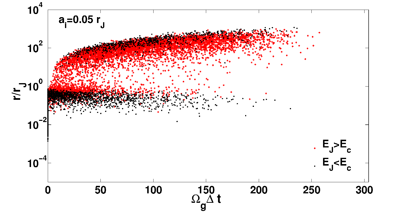
We expect that the sooner the binary is disrupted—in the sense that kicks from passing stars cause the Jacobi constant to random walk to a value exceeding $E_{c}$ —the larger the separation of the binary system will be at the time $10\,\mbox{Gyr}$ . We label the interval since the Jacobi constant of the binary first exceeded $E_{c}$ until $10\,\mbox{Gyr}$ (the “escape age”) as $\Delta t$ (if the Jacobi constant never exceeds $E_{c}$ we set $\Delta t=0$ ). The relation between the separation at $10\,\mbox{Gyr}$ and the escape age is shown in Figure 5. The red points have $E_{J}>E_{c}$ at $10\,\mbox{Gyr}$ while the black points have $E_{J}<E_{c}$ . As noted earlier in Figures 3 and 4, there is a gap around the separation $5r_{J}$ in each panel. The black points with $\Delta t>0$ had $E_{J}>E_{c}$ at some point in their history, but subsequent perturbations kicked them back to $E_{J}<E_{c}$ (black points with $r\gtrsim r_{J}$ must lie in regions B or C in Figure 1). The black points along the axis $\Delta t=0$ never escaped, i.e., $E_{J}<E_{c}$ for the entire integration. For the binary stars with separation $r\gg r_{J}$ , the general trend is that the sepration grows with $\Delta t$ . The upper envelope of the points in Figure 5 is roughly $r\propto(\Delta t)^{\alpha}$ with $\alpha=1.4$ –1.5. This behavior has a simple physical explanation: the relative velocity random walks due to stellar perturbations and therefore grows as $v\propto(\Delta t)^{1/2}$ , so the separation grows as $r\sim v\Delta t\propto(\Delta t)^{1.5}$ .

The relative velocity $v$ and separation $r$ of the binary systems at the end of the simulation are shown in Figure 6. The red dotted line is the zero-energy line for Keplerian orbits, $v^{2}/2=G(M_{1}+M_{2})/r$ . In the top four panels, binary stars with separation $r$ much less than the initial semi-major axis $a_{i}$ follow this line quite closely, since they are generally found at $r\ll a_{i}$ only when they are near the pericenter of near-parabolic orbits. In the bottom two panels, the binaries follow the zero-energy line closely when $r\ll 0.001r_{J}$ , the lower cutoff to the semi-major axis range in the assumed initial Öpik distribution. As the separation increases, to $\sim r_{J}$ , the typical velocity decreases but the logarithmic spread in velocities grows, as shown by the green error bars.

In Figure 7 we plot the relation between the RMS line-of-sight relative velocity and projected separation, as seen from an observer with a random orientation. Different initial semi-major axes yield almost the same curve. When the separation is $\lesssim r_{J}$ , the relative velocity decreases with increasing separation as $r_{p}^{-1/2}$ , as one would expect for Keplerian motion. When the separation is larger than $r_{J}$ , the RMS relative velocity increases with increasing separation. The minimum RMS line-of-sight relative velocity is $\sim\Omega_{g}r_{J}$ .

The maximum relative velocity for separations $\gg r_{J}$ is a few times $\Omega_{g}r_{J}\simeq 0.05\,\mbox{km s}^{-1}$ (eq. 44), two orders of magnitude smaller than the typical relative velocity between unrelated stars in the solar neighborhood. Because of this, surveys that provide accurate velocity data have far greater ability to identify binaries with $r\gg r_{J}$ than surveys with only positions⁵⁵ 5 D. Fabrycky points out that unbound pairs of asteroids, possibly formed by collisional disruption of large parent asteroids in the past, have been detected by similar techniques [36].. To illustrate this, in Figure 8 we plot the indicative phase-space density (number density divided by $\langle v^{2}\rangle^{3/2}$ ) of companions from our simulations, which contain 50,000 binary stars at birth. If a fraction $f$ of stars are found in wide binaries, the total number of stars in a catalog that is required to obtain 50,000 wide binaries is $1\times 10^{5}/f$ . The horizontal line shows the analogous indicative phase-space density of field stars in the solar neighborhood, $\rho_{0}/\langle v^{2}\rangle^{3/2}$ where $\rho_{0}$ is given by equation (47) and $\langle v^{2}\rangle=3\sigma^{2}$ with $\sigma=40\,\mbox{km s}^{-1}$ as derived in §III.1. The phase-space density of binaries exceeds the density of field stars out to separations of $\sim 10^{2}r_{J}$ or well over $100\,\mbox{pc}$ . Thus a statistical measurement of the distribution of binaries at $\sim 100\,\mbox{pc}$ separation can be achieved by a survey such as GAIA that is (i) large enough to contain $\gtrsim 10^{5}$ stars that were originally in wide binaries; (ii) accurate enough that the errors in distance and velocity are smaller than the separations and relative velocities ( $\sim 100\,\mbox{pc}$ and $0.1$ – $0.2\,\mbox{km s}^{-1}$ ).

IV Discussion and conclusions

We have studied the evolution and disruption of wide binary stars under the gravitational influence of passing field stars. There have been many treatments of this problem already (see the Introduction for references) but most of these (i) ignore the Galactic tidal field; (ii) define the binary to be “disrupted” when the Keplerian energy becomes positive or when the separation exceeds the Jacobi or tidal radius, and assume that the stars disappear instantaneously once they are disrupted. The novel features of our treatment are that we include the effects of the Galactic tidal field and follow the evolution of the stars after they are disrupted.

Our simulations show that the usual treatment of binary disruption is oversimplified. In particular,

•

The number of binaries does not drop to zero when the separation exceeds the Jacobi radius $r_{J}$ ; rather there is a minimum in the density (number per unit log separation) at a few times $r_{J}$ , almost independent of the initial semi-major axis distribution. Interior to this minimum there is a peak in the density due to the binaries that have not yet escaped, and exterior there is a peak due to binaries that are slowly drifting apart (Figure 3).
•

Many binaries that have achieved escape energy (more precisely, that have Jacobi constants that exceed the critical value $E_{c}$ defined in eq. 22) remain at separations less than the Jacobi radius for many Gyr, either because they are on stable orbits that do not escape to infinity or because subsequent perturbations from passing stars bring their Jacobi constant back below $E_{c}$ before they have time to escape (Figs. 4 and 5).
•

Because the escaped binary components have small relative velocities, they contribute strongly to the phase-space correlation function in the solar neighborhood. Large astrometric surveys that can measure three-dimensional distances and velocities to sufficient accuracy ( $\sim 100\,\mbox{pc}$ and $0.1$ – $0.2\,\mbox{km s}^{-1}$ ) can detect this correlation signal out to hundreds of parsecs.

These calculations could be improved in several ways. Our simulations do not include perturbations from passing molecular clouds, which are comparable to the perturbations from passing stars at $a\sim 0.1\,\mbox{pc}$ within the uncertainties [19, 39, 25]. Moreover the qualitative effects of molecular clouds may be different because the impact parameter of the most important cloud encounters is much larger than the binary’s Jacobi radius, whereas the most important stellar encounters have impact parameters smaller than the Jacobi radius. Molecular clouds have a much smaller scale height than old stars, so the effects of passing clouds and stars may be disentangled observationally by examining variations in the binary distribution with the vertical amplitude of the center-of-mass motion of the binaries [34].

The use of the central limit theorem to model stellar kicks as a Gaussian distribution (eq. 34) is a plausible first approximation but should eventually be replaced by a Monte Carlo model of the kicks from individual passing stars. As described in the discussion following equation (53) the assumption that there are many kicks per interval $\Delta t_{p}$ is not correct at small semi-major axes. Also, for orbits near the critical Jacobi constant $E_{c}$ there may be chaotic phenomena such as resonance sticking that can only be modeled using the actual distribution of velocity kicks [12, 16, 11]. Despite these concerns, the tests we have carried out in §III.1 suggest that our results are not sensitive to the specific value of $\Delta t_{p}$ .

The distinction between evolution due to the Galactic tidal field (§II.1) and evolution due to impulsive kicks (§II.2) is artificial, since the same stars in the disk contribute both the tidal field (apart from a contribution from dark matter) and the kicks (apart from a contribution from molecular clouds). The approximation that there is a static tidal field can be misleading on timescales less than the collision time (51); however, we do not believe that this approximation has biased our results significantly. See [17] and [9] for further discussions of this issue.

There is a large literature on tidal tails from star clusters [26, 4, 13, 22, e.g.,]. These differ from the binary-star tails discussed here in several ways. Most obviously, clusters contain many stars so the structure of the tail from a single cluster can be mapped in great detail; in contrast, the tail from a single binary contains only two stars so we must combine many binaries to measure the tail properties. A second difference is that the kicks to the orbits of stars in a cluster arise from other cluster stars, and therefore cease once the star escapes from the cluster, whereas the kicks to a binary arise from passing stars and continue after disruption. The most important consequence of this difference is that the length of a cluster tidal tail grows $\propto t$ , while a binary-star tail grows $\propto t^{1.5}$ .

Our results hold only for disk binary stars but it is straightforward to repeat the calculation for halo binaries. These are of particular interest because the semi-major axis distribution of halo binaries can be used to constrain the mass distribution of compact objects in the dark halo [41, 31].

We thank Dan Fabrycky, Mario Jurić, and Yue Shen for helpful discussions. We also thank the referee, Winston Sweatman, for comments that significantly improved the paper. This research was supported in part by NASA grant NNX08AH83G, and used computational facilities supported by NSF grant AST-0216105.

Appendix A Diffusion of the escaped binary stars

Here we give an approximate analytic treatment of our results, by solving for the evolution of binary stars with $r\ll r_{J}$ and $r\gg r_{J}$ separately, then matching the two solutions at $r_{J}$ .

The behavior of binary stars with separation much smaller than $r_{J}$ can be described by the diffusion approximation given in §II.3. The probability $p_{e}(\tau)d\tau$ for the binary stars to escape in the time interval $(\tau,\tau+d\tau)$ ⁶⁶ 6 The initial time is set to be zero. is (derivative of eq. B19 in Weinberg et al. 39, or from eq. 40 as $|E_{1}|\rightarrow 0$ )

p_{e}(\tau)=\frac{4}{3\sqrt{\pi}}\frac{h_{0}^{5/2}}{\tau^{7/2}}e^{-h_{0}/\tau}.

(A1)

After the stars have escaped to $r\gg r_{J}$ , the gravitational force between the two stars is much smaller than the Galactic tidal force. Then the relative motion in the absence of kicks is described by equations (19) with the right side set to zero. Moreover their separations are dominated by drift along the azimuthal or $y$ direction, as seen from Figure 2, so $r\simeq y$ . As the amplitude of the epicycle motion is small compared to $y$ , we have $y\approx y_{g}$ , where $y_{g}$ is the position of the guiding center of the relative motion (cf. the analogous equations 17 for the motion of the center of mass). Therefore we must determine the equation that governs the evolution of $y_{g}$ in the presence of kicks from passing stars.

The relation between the velocity of the guiding center $v_{g}=\dot{y}_{g}$ and the relative position and velocity $(x,y,v_{x},v_{y})$ is

v_{g}=-\frac{A_{g}}{A_{g}-\Omega_{g}}(v_{y}+2\Omega_{g}x).

(A2)

This can be verified or derived from the epicycle equations for the relative motion (the analogs of eqs. 17 for the center of mass epicycle motion) or from equations (8.101) and (8.102) of [5], which relate the orbital parameters and the phase-space coordinates to the energy and angular momentum in the epicycle approximation.

With equation (A2 and the impulse approximation for the kick, the diffusion coefficient for $v_{g}$ is given by

D[(\Delta v_{g})^{2}]=2\left(\frac{A_{g}}{A_{g}-\Omega_{g}}\right)^{2}D[(\Delta v_{y})^{2}].

(A3)

The factor of two arises because kicks on both stars contribute to the diffusion of $v_{g}$ .

Let $f(t,y_{g},v_{g})dy_{g}dv_{g}$ be the probability that the escaped binary stars lie in the interval $(y_{g},y_{g}+dy_{g})$ and $(v_{g},v_{g}+dv_{g})$ at time $t$ . Then the distribution function $f(t,y_{g},v_{g})$ satisfies the simplified Fokker-Planck equation

\frac{\partial f}{\partial t}+v_{g}\frac{\partial f}{\partial y_{g}}=\frac{1}{2}D[(\Delta v_{g})^{2}]\frac{\partial^{2}f}{\partial v_{g}^{2}}.

(A4)

Here we have neglected the term $D[\Delta v_{g}]\partial f/\partial v_{g}$ because $\partial f/\partial v_{g}$ is small compared to $\partial^{2}f/\partial v_{g}^{2}$ . The diffusion coefficient $D[(\Delta v_{y})^{2}]$ for either star is given by equation (30), which is now⁷⁷ 7 The subscript $i$ for the diffusion coefficients in equation (30) is omitted here.

D[(\Delta v_{y})^{2}]=\frac{v_{y}^{2}}{v^{2}}D[(\Delta v_{||})^{2}]+\frac{v_{x}^{2}+v_{z}^{2}}{2v^{2}}D[(\Delta v_{\perp})^{2}].

(A5)

For binary stars with large separation, the velocity $v$ is much smaller than $\sigma$ . In this case, we have $D[(\Delta v_{\perp})^{2}]=2D[(\Delta v_{||})^{2}]$ and thus $D[(\Delta v_{y})^{2}]=D[(\Delta v_{||})^{2}]$ . Then from equations (31) and (A3)

D[(\Delta v_{g})^{2}]=\left(\frac{A_{g}}{A_{g}-\Omega_{g}}\right)^{2}\frac{16\sqrt{2\pi}G^{2}\rho_{2}\ln\wedge}{3\sigma}.

(A6)

Note that the diffusion coefficient is independent of $y_{g}$ and $v_{g}$ so we may label a constant $D_{g}\equiv D[(\Delta v_{g})^{2}]$ . With the initial condition $f(0,y_{g},v_{g})=\delta(y_{g})\delta(v_{g})$ and the boundary condition that $f\rightarrow 0$ when $y_{g}\rightarrow\infty$ or $v_{g}\rightarrow\infty$ , the solution to equation (A4) is

f(t,y_{g},v_{g})=\frac{\sqrt{3}}{\pi D_{g}t^{2}}\mbox{exp}\left[-\frac{6y_{g}^{2}}{D_{g}t^{3}}+\frac{6y_{g}v_{g}}{D_{g}t^{2}}-\frac{2v_{g}^{2}}{D_{g}t}\right].

(A7)

The marginal probability distribution of $y_{g}$ can be gotten by integration over $v_{g}$ , which yields

f(t,y_{g})=\int dv_{g}\,f(t,y_{g},v_{g})=\sqrt{\frac{3}{2\pi D_{g}t^{3}}}\mbox{exp}\left[-\frac{3}{2}\frac{y_{g}^{2}}{D_{g}t^{3}}\right].

(A8)

Then at the final time $t_{f}=10$ Gyr, the probability that the binary has separation $(y_{g},y_{g}+dy_{g})$ ] is

p_{f}(y_{g})dy_{g}=dy_{g}\int_{0}^{t_{f}}p_{e}(t)f(t_{f}-t,y_{g})dt,

(A9)

where $p_{e}(t)=p_{e}(\tau)d\tau/dt$ is given by (A1).

We compare the probability distribution (A9) to the escaped binary stars from our simulations in Figure 9 (because the maximum impact parameter $b_{\rm{max}}$ is chosen to be the half separation of the binary system at each kick time, which is different at different times, we have to choose a “mean” $b_{\rm{max}}$ when we use equation (A9) to fit the simulation data). We can see that the analytic treatment works quite well at the largest separations, and works better if the initial semi-major axis is larger. At small separations the fit is less good, presumably because our approximation that the gravitational force between the stars is negligible compared to the tidal force is not accurate.

References

[1] Ambartsumian, V. 1937, Astr. Zh., 14, 207
[2] Bahcall, J. N., & Soneira, R. M. 1981, ApJ, 246, 122
[3] Bahcall J. N., Hut P., & Tremaine S. 1985, AJ, 290, 15
[4] Belokurov, V., Evans, N. W., Irwin, M. J., Hewett, P. C., & Wilkinson, M. I. 2006, ApJ, 637, L29
[5] Binney J. J., & Tremaine S. 2008, Galactic Dynamics (2nd ed.; Princeton: Princeton University Press)
[6] Chanamé, J., & Gould A. 2004, ApJ, 601, 289
[7] Chanam $\acute{\rm{e}}$ , J. 2007, in IAU Symposium 240, Binary Stars as Critical Tools and Tests in Contemporary Astrophysics, ed. W. I. Hartkopf et al. (Cambridge: Cambridge University Press), 316
[8] Chandrasekhar, S. 1944, ApJ, 99, 54
[9] Collins, B. F., & Sari, R. 2009, in preparation
[10] Dehnen, W., & Binney, J. J. 1998, MNRAS, 298, 387
[11] Ernst, A., Just, A., Spurzem, R., & Porth, O. 2008, MNRAS, 383, 897
[12] Fukushige, T., & Heggie, D. C. 2000, MNRAS, 318, 753
[13] Grillmair, C. J., & Dionatos, O. 2006, ApJ, 643, L17
[14] Heggie, D. C. 1975, MNRAS, 173, 729
[15] Heggie, D. C. 1977, Revista Mexicana de Astronomia y Astrofisica, 3, 169
[16] Heggie, D. C. 2001, in The Restless Universe, ed. B. A. Steves and A. J. Maciejewski, 109 (also arXiv:astro-ph/0011294)
[17] Heisler, J., & Tremaine, S. 1986, Icarus, 65, 13
[18] Hénon, M. 1970, A&A, 9, 24
[19] Hut, P., & Tremaine, S. 1985, AJ, 90, 1548
[20] King, I. R. 1977, Revista Mexicana de Astronomia y Astrofisica, 3, 167
[21] Kroupa, P., Tout, C. A., & Gilmore, G. 1993, MNRAS, 262, 545
[22] Küpper, A.H.W., Macleod, A., & Heggie, D. C. 2008, MNRAS, 387, 1248
[23] Latham, D. W., Davis, R. J., Stefanik, R. P., Mazeh, T., & Abt, H. A. 1991, AJ, 101, 625
[24] Lépine, S., & Bongiorno, B. 2007, AJ, 133, 889
[25] Mallada, E., & Fernandez, J. A. 2001, Revista Mexicana de Astronomia y Astrofisica Conference Series, 11, 27
[26] Odenkirchen, M., et al. 2001, ApJ, 548, L165
[27] Öpik, E. J. 1924, Tartu Obs. Publ., 25
[28] Öpik, E. J. 1932, Proc. Am. Acad. Sci., 67, 169 (Harvard College Obs. Reprint No. 79)
[29] Palasi, J. 2000, in IAU Symposium 200, The Formation of Binary Stars, ed. B. Reipurth and H. Zinnecker, 145
[30] Poveda, A., Allen, C., & Hernández-Alcántara, A. 2007, in IAU Symposium 240, Binary Stars as Critical Tools and Tests in Contemporary Astrophysics, ed. W. I. Hartkopf et al. (Cambridge: Cambridge University Press), 240, 417
[31] Quinn, D. P., Wilkinson, M. I., Irwin, M. J., Marshall, J., Koch, A., & Belokurov, V. 2009, MNRAS, 396, L11
[32] Retterer, J. M., & King, I. R. 1982, ApJ, 254, 214
[33] Shen, Y., & Tremaine, S. 2008, AJ, 136, 2453
[34] Sesar, B., Ivezić, Ž., & Jurić, M. 2008, ApJ, 689, 1244
[35] Stiefel, E. L., & Scheifele, G. 1971, Linear and Regular Celestial Mechanics (Berlin: Springer-Verlag)
[36] Vokrouhlický, D., & Nesvorný, D. 2008, AJ, 136, 280
[37] Wasserman, I., & Weinberg, M. D. 1987, ApJ, 312, 390
[38] Wasserman, I., & Weinberg, M. D. 1991, ApJ, 382, 149
[39] Weinberg, M. D., Shapiro, S. L., & Wasserman, I. 1987, ApJ, 312, 367
[40] Yabushita, S. 1966, MNRAS, 133, 133
[41] Yoo, J., Chanamé, J., & Gould A. 2004, ApJ, 601, 311