In 1978 Fisher and de Gennes [1] realized that when thermal fluctuations are restricted by a container a force acts on the walls of the container. Since this effect is rather similar to the Casimir effect, where the restriction of quantum fluctuations induces a force, it is called “thermodynamic” Casimir effect. Since thermal fluctuations only extend to large scales in the neighbourhood of a continuous phase transitions it is also called “critical” Casimir effect. Recently this effect has attracted much attention, since it could be verified for various experimental systems and quantitative predictions could be obtained from Monte Carlo simulations of spin models [2].

In the thermodynamic limit of the three dimensional system, the correlation length, which measures the spatial extension of fluctuations, diverges following the power law

where $t=(T-T_{c})/T_{c}$ is the reduced temperature and $T_{c}$ the critical temperature. $\xi_{0,+}$ and $\xi_{0,-}$ are the amplitudes of the correlation length in the high and low temperature phase, respectively. While $\xi_{0,+}$ and $\xi_{0,-}$ depend on the microscopic details of the system, the critical exponent $\nu$ and the ratio $\xi_{0,+}/\xi_{0,-}$ are universal. At the critical point also other quantities like the specific heat show a singular behaviour:

In the case of the XY universality class that we consider here, the exponent $\alpha=-0.151(3)$ [3] of the specific heat is negative. Therefore the analytic background $B$ has to be taken into account. Note that the critical exponents of the correlation length and the specific heat are related by the hyperscaling relation $\alpha=2-d\nu$, where $d$ is the dimension of the system. For reviews on critical phenomena and its modern theory, the Renormalization Group, see e.g. [4, 5, 6, 7].

The singular behaviour at the critical point originates from the fact that thermal fluctuations range over all length scales. Therefore the behaviour in the neighbourhood of the critical point is modified if the system is confined by a container. A priori thermodynamic quantities are functions of the reduced temperature and the size $L_{0}$ of the container, assuming a fixed geometry. However the theory of finite size scaling ¹¹ 1 For a review on finite size scaling see [8]. predicts that the physics of the system is governed by the ratio $L_{0}/\xi$ as long as $L_{0},\xi\gg a$, where $a$ is the microscopic scale of the system. In particular if a quantity in the thermodynamic limit behaves as $A\simeq a_{0,\pm}|t|^{-w}$, finite size scaling predicts that $A(L_{0},t)\simeq L_{0}^{w/\nu}\tilde{g}(L_{0}/\xi)$, where $w$ is the critical exponent of $A$ and $\xi$ the correlation length of the bulk system. We can rewrite this equation as

by using (1), which is the form used in the following. Note that the function $g$ depends on the details of the container. For example for a cube it is different from a thin film. It also depends on the type of boundary conditions that is imposed by the walls of the container on the order parameter of the system.

The predictions of finite size scaling theory have been tested in experiments and theoretical studies for various universality classes and confining geometries; for reviews see [8, 9]. Here we shall focus on thin films in the three dimensional XY universality class, which is shared by the $\lambda$-transition of ⁴He. Very precise experimental results for critical exponents and universal amplitude ratios were obtained for this phase transition [10]. Also a large number of experiments on thin films of ⁴He and ³He-⁴He mixtures were performed to probe finite size scaling [11]. In particular the specific heat $C$ of thin films has been studied. The excess specific heat should behave as

The reason to study the excess specific heat rather than just the specific heat $C(L_{0},t)$ is to cancel the analytic background $B$. Note that the scaling function $f_{2}(x)$ of the excess specific heat is, up to a constant factor, the second derivative $h^{\prime\prime}(x)$ of the scaling function $h(x)$ of the excess free energy per area

where $\tilde{f}_{film}(L_{0},t)$ is the free energy per area of the thin film, $\tilde{f}_{bulk}(t)$ the free energy density of the bulk system, $d=3$ the dimension of the system and $x=t[L_{0}/\xi_{0}]^{1/\nu}$. Note that in the case of thin films we consider, following the literature on the thermodynamic Casimir effect, free energies per area. We hope that this does not lead to confusion, since in the case of the specific heat, energies per volume are considered.

From a thermodynamic point of view, the Casimir force per unit area is given by

where $L_{0}$ is the thickness of the film. Inserting the finite size scaling ansatz (5) for the excess free energy into (6) we get

where

This relation is well known and can be found e.g. in [14]. We like to emphasis, that it is at the very heart of finite size scaling that the behaviour of the Casimir force, which gives the reaction of the film with respect to a change of the thickness and the excess specific heat which gives the reaction of the film with respect to a change of the temperature are given by the same scaling function $h(x)$ of the excess free energy.

The purpose of the present work is to compute the finite size scaling function $\theta(x)$ by using the energy density of thin films obtained from Monte Carlo simulations of a lattice model [15] and by using experimental data for the specific heat of thin films of ⁴He near the $\lambda$-transition [16, 17].

As a preliminary study, we simulate $L^{3}$ systems with periodic boundary conditions in all directions. In order to eliminate leading corrections to scaling we have used the improved two component $\phi^{4}$ model on the simple cubic lattice. For a precise definition of the model see section 2. Using the results obtained for the energy density for a dense grid of temperatures in the neighbourhood of the critical point, we investigate the scaling behaviour and compute the finite size scaling functions $h^{\prime}(x)$ and $h(x)$. We find that corrections to scaling are small for the lattices sizes $L=8$, $16$ and $32$ that we have simulated.

In the case of thin films we analyse data for the energy density that were obtained in [15] from simulations of the improved two component $\phi^{4}$ model on the simple cubic lattice. In [15] these data where used to compute the specific heat. In order to get a vanishing order parameter as it is observed at the boundaries of ⁴He films, Dirichlet boundary conditions with vanishing field were imposed. In singular quantities these lead to corrections $\propto L_{0}^{-1}$ [18], which can be expressed by an effective thickness $L_{0,eff}=L_{0}+L_{s}$. In [19] we find $L_{s}=1.02(7)$ for the model that we consider here. Note that the boundary conditions also effect the analytic background of the specific heat and the energy density, which also leads to corrections $\propto L_{0}^{-1}$. However it turns out that these corrections are not given by the same $L_{0,eff}$ as for the singular quantities. Taking into account these subtleties we arrive at accurate result for $h^{\prime}(x)$, $h(x)$ and $\theta(x)$. In particular for $\theta(x)$ in the range $-15\lessapprox x\lessapprox 4$ we find a good match with our previous result [20] ²² 2 In [20] we have compared our result for $\theta(x)$ with previous ones obtained from simulations of the XY model [21, 22] and experiments on thin films of ⁴He [12, 13]; overall we find a reasonable agreement., where we computed the Casimir force by taking the derivative of the excess free energy with respect to the thickness $L_{0}$ of the film.

Next we compute $\theta(x)$ by using experimental results for the excess specific heat obtained from experiments on thin films of ⁴He [16, 17]. Even though this is a quite simple exercise, to our knowledge, it has not been done before. For $-5\lessapprox x\lessapprox 4$ we find a reasonable match with our result [20]. However in the low temperature phase, for $x\lessapprox-5$ we get results that strongly deviate from [20] and can be ruled out by plausibility. This corroborates the observation that in the low temperature phase for $x\lessapprox-5$ the excess specific heat does not scale well [11].

This paper is organized as follows: First we define the model and the observables that we consider. Next we discuss the finite size scaling behaviour of the free energy density. In particular, we discuss corrections to scaling caused by Dirichlet boundary conditions. In section 4 we compute the scaling functions $h^{\prime}(x)$ and $h(x)$ for $L^{3}$ systems with periodic boundary conditions. Then in section 5 we compute $h^{\prime}(x)$, $h(x)$ and $\theta(x)$ using the data for the energy density of thin films with Dirichlet boundary conditions obtained in [15]. The result for $\theta(x)$ is compared with the one that we [20] obtained directly from the thermodynamic Casimir force. Next in section 6 we compute $\theta(x)$ starting from data for the excess specific heat of films of ⁴He in the neighbourhood of the $\lambda$-transition. Finally we summarize and conclude.

We study the two component $\phi^{4}$ model on the simple cubic lattice. We label the sites of the lattice by $x=(x_{0},x_{1},x_{2})$. The components of $x$ might assume the values $x_{i}\in\{1,2,\ldots,L_{i}\}$. In this work we have performed simulations of lattices with $L_{0}=L_{1}=L_{2}$ and periodic boundary conditions in all three directions. Furthermore we analyse data obtained in [15] for thin films. In this case lattices of the size $L_{1}=L_{2}=L$ and $L_{0}\ll L$ are studied. In 1 and 2-direction periodic boundary conditions and free boundary conditions in 0-direction are employed. This means that the sites with $x_{0}=1$ and $x_{0}=L_{0}$ have only five nearest neighbours. This type of boundary conditions could be interpreted as Dirichlet boundary conditions with $0$ as value of the field at $x_{0}=0$ and $x_{0}=L_{0}+1$. Note that viewed this way, the thickness of the film is $L_{0}+1$ rather than $L_{0}$. This provides a natural explanation of the result $L_{s}=1.02(7)$ obtained in [19]. The Hamiltonian of the two component $\phi^{4}$ model, for a vanishing external field, is given by

where the field variable $\vec{\phi}_{x}$ is a vector with two real components. $<x,y>$ denotes a pair of nearest neighbour sites on the lattice. The partition function is given by

Note that following the conventions of our previous work, e.g. [23], we have absorbed the inverse temperature $\beta$ into the Hamiltonian. ³³ 3 Therefore, following [6] we actually should call it reduced Hamiltonian. In the limit $\lambda\rightarrow\infty$ the field variables are fixed to unit length; i.e. the XY model is recovered. For $\lambda=0$ we get the exactly solvable Gaussian model. For $0<\lambda\leq\infty$ the model undergoes a second order phase transition that belongs to the XY universality class. Numerically, using Monte Carlo simulations and high-temperature series expansions, it has been shown that there is a value $\lambda^{*}>0$, where leading corrections to scaling vanish. Numerical estimates of $\lambda^{*}$ given in the literature are $\lambda^{*}=2.10(6)$ [24], $\lambda^{*}=2.07(5)$ [23] and most recently $\lambda^{*}=2.15(5)$ [3]. The inverse of the critical temperature $\beta_{c}$ has been determined accurately for several values of $\lambda$ using finite size scaling (FSS) [3]. We shall perform our simulations at $\lambda=2.1$, since for this value of $\lambda$ comprehensive Monte Carlo studies of the three-dimensional system in the low and the high temperature phase have been performed [19, 3, 25, 26]. At $\lambda=2.1$ one gets $\beta_{c}=0.5091503(6)$ [3]. Since $\lambda=2.1$ is not exactly equal to $\lambda^{*}$, there are still corrections $\propto L^{-\omega}$, although with a small amplitude. In fact, following [3], it should be by at least a factor 20 smaller than for the standard XY model.

In [19] we find for $\lambda=2.1$ by fitting the data for the second moment correlation length in the high temperature phase $\xi_{2nd}\simeq 0.26362(8)t^{-0.6717}$, where $t=0.5091503-\beta$. We shall use this definition of the reduced temperature also in the following discussion of our numerical results; Hence $\xi_{0}=0.26362(8)$. Note that in the high temperature phase there is little difference between $\xi_{2nd}$ and the exponential correlation length $\xi_{exp}$ which is defined by the asymptotic decay of the two-point correlation function. Following [23] $\lim_{t\searrow 0}\frac{\xi_{exp}}{\xi_{2nd}}=1.000204(3)$ for the thermodynamic limit of the three-dimensional system. Hence at the level of precision reached here it does not matter whether $\xi_{0,exp}$ or $\xi_{0,2nd}$ is used in the scaling variable $x=t[L_{0}/\xi_{0}]^{1/\nu}$.

Let us briefly discuss the scaling behaviour of the reduced excess free energy per area. Since we study an improved model we ignore corrections $\propto L_{0}^{-\omega}$ in the following. We take into account leading corrections due to the boundary conditions by replacing the thickness $L_{0}$ of the film by $L_{0,eff}=L_{0}+L_{s}$ at the appropriate places. We split the free energies in singular (s) and non-singular (ns) parts:

where

is a universal finite size scaling function and $x=t[L_{0,eff}/\xi_{0}]^{1/\nu}$. Following RG theory the non-singular part is not affected by finite size effects. However it is not clear a priori how Dirichlet boundary conditions affect the non-singular part of the free energy. Therefore we allow for $L_{sns}=L_{0,eff,ns}-L_{0}\neq 0$ and $L_{sns}\neq L_{s}$. Taking the derivative with respect to $L_{0}$ we get the thermodynamic Casimir force per area [14]

where

Note that the boundary terms $L_{s}f_{bulk,s}$ and $L_{sns}f_{ns}$ do not contribute to the Casimir force.

First we have studied a finite lattice with $L=L_{0}=L_{1}=L_{2}$ with periodic boundary conditions in all directions. This way we avoid corrections caused by the free boundary conditions and possible difficulties related with the Kosterlitz-Thouless transition of thin films. In our simulations we determine the energy density $E$ for the lattice sizes $L=8$, $16$ and $32$ for a large number of $\beta$-values in the neighbourhood of the critical temperature. In particular, we have simulated at 159 $\beta$-values in the interval $0.35\leq\beta\leq 0.58$, 205 $\beta$-values in the interval $0.35\leq\beta\leq 0.58$ and 161 $\beta$-values in the interval $0.45\leq\beta\leq 0.535$ in the case of $L=8$, $16$ and $32$, respectively. For most of these simulations we performed $10^{6}$ measurements. For each of these measurements we performed one Metropolis sweep, two overrelaxation sweeps and a number of single cluster [27] updates. The number of single cluster updates is chosen such that the number of updates times the average size of a cluster roughly equals $L^{3}$. As random number generator we have used the SIMD-oriented Fast Mersenne Twister algorithm [28]. In total we have used about 3 weeks of CPU-time on a single core of a Quad-Core Opteron(tm) 2378 CPU (2.4 GHz). In order to compute the excess energy density

we have used the results for $E_{bulk}(t)$ obtained in section 4.1 of [15].

The reduced excess free energy density behaves as

where $x=t[L/\xi_{0}]^{1/\nu}$. It follows for the excess energy density

Since we study an improved model and periodic boundary conditions in all directions, we expect that analytic corrections are leading. In figure 1 we plot $[L/\xi_{0}]^{-1/\nu}L^{3}[E(t,L)-E_{bulk}(t)]$ as a function of $t[L/\xi_{0}]^{-1/\nu}$. The curves for $L=8$, $16$ and $32$ fall nicely on top of each other, showing that corrections to scaling are numerically small. The excess energy is positive for all temperatures. At $x\approx-0.3$ the function assumes a maximum. The value at the maximum is $\approx 0.295$. In the high temperature phase, for increasing $x$ the function $h^{\prime}(x)$ rapidly approaches zero. In contrast, in the low temperature phase it is only slowly approaching zero with decreasing $x$. This behaviour might be explained by the presence of a Goldstone mode in the low temperature phase.

Next we have computed the excess free energy using eq. (14). To this end we integrated our data for the excess energy by using the trapezoidal rule. We have started the integration at $\beta_{0}=0.35$, $0.45$ and $0.49$ for $L=8$, $16$ and $32$, respectively. At these values of $\beta_{0}$ the deviation of the excess energy from zero is of similar size as the statistical error. In figure 2 we plot $L^{3}[f(t,L)-f_{bulk}(t)]$ as a function of $t[L/\xi_{0}]^{-1/\nu}$. As one should expect, the curves for $L=8$, $16$ and $32$ fall nicely on top of each other. Since the excess energy is positive for all values of $x$, the excess free energy is monotonically increasing with increasing $x$. At the critical point the scaling functions assumes the value $h(0)=-1.162(4)$.

In Fig. 6 of [29] results for an isotropic $L^{3}$ system with periodic boundary conditions for the Ising universality class and the limit $n\rightarrow\infty$ of $O(n)$ symmetric models are given. The Ising result is obtained from a perturbative approach in three dimensions fixed, while the $n\rightarrow\infty$ result is exact. In the Ising case, $h(x)$ shows a minimum in the low temperature phase, while for $n\rightarrow\infty$ it is monotonically decreasing as the temperature decreases. Hence qualitatively the behaviour for $n=2$, studied here, is the same as for $n\rightarrow\infty$.

Here we study thin films with free boundary conditions in the short direction. This geometry is relevant for the comparison with experimental results obtained for thin films of ⁴He. Most of the Monte Carlo data are taken from our previous work [15, 20], where we have simulated films of the thicknesses $L_{0}=8$, $16$ and $32$. Therefore we refrain from giving the details of the simulations and refer the reader to [15, 20].

Analogous to the previous section we compute the scaling function $h^{\prime}(x)$ of the excess energy density and $h(x)$ of the excess free energy density. Using these we obtain the scaling function $\theta(x)=2h(x)-\frac{x}{\nu}h^{\prime}(x)$ of the thermodynamic Casimir force.

In [15] we have taken great care to get the deviations of the energy density from its effectively two dimensional thermodynamic limit under control. In order to achieve this, quite large ratios $L_{1}/L_{0}$ are needed in the neighbourhood of the peak of the specific heat. In the case of $L_{0}=8$ we have simulated lattices of a size up to $L_{1}=L_{2}=2048$, and for $L_{0}=16$ up to $L_{1}=L_{2}=1800$. For $L_{0}=32$ we have skipped the interval $0.5136<\beta<0.516$, since we could not simulate sufficiently large values of $L_{1}=L_{2}$.

In figure 3, similar to the previous section, we have plotted $E_{ex}L_{0}^{2}[L_{0}/\xi_{0}]^{-1/\nu}$ versus $t[L_{0}/\xi_{0}]^{1/\nu}$, where now

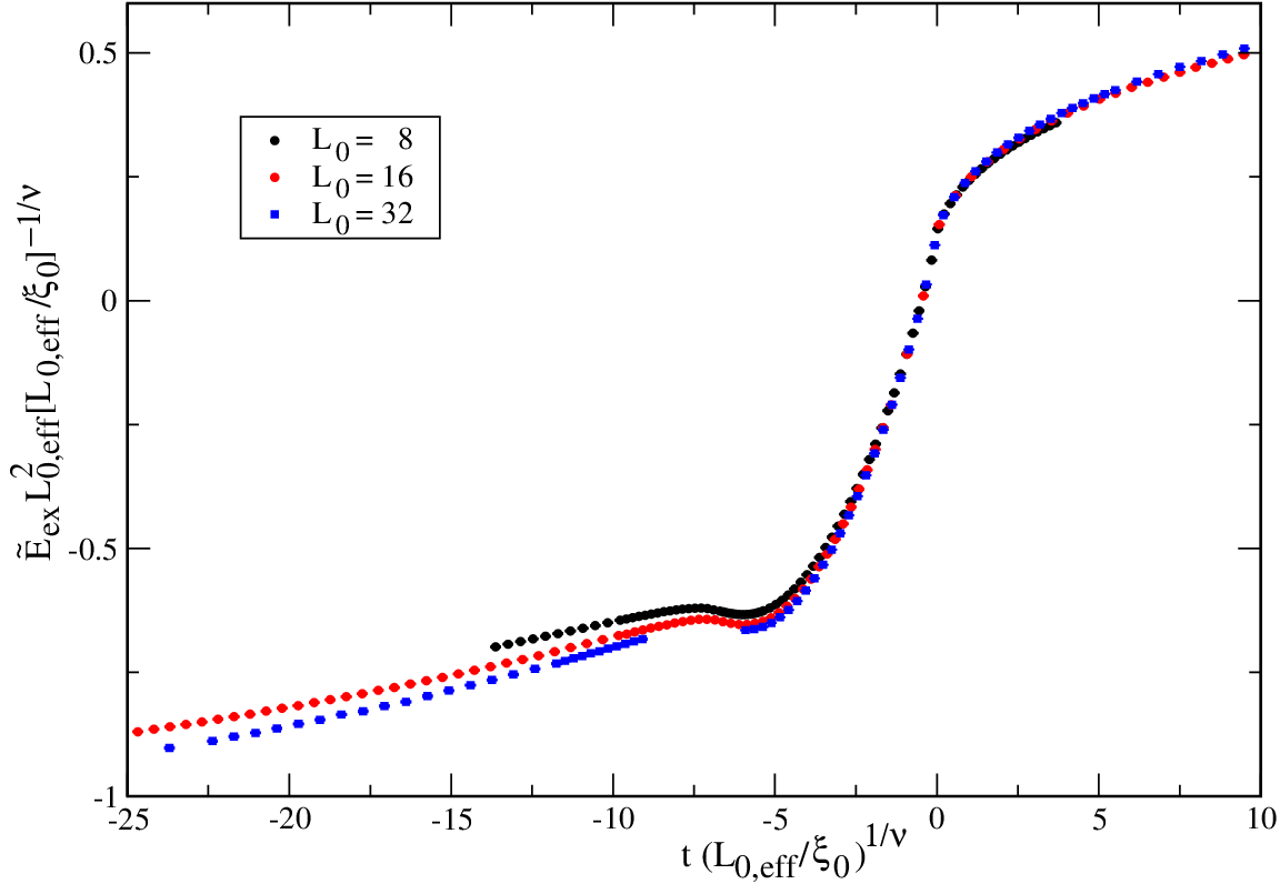
is the excess energy per area. In contrast to the previous section we find that there is a huge discrepancy between the three curves. The dominant effect seems that the curves are shifted by a constant with respect to each other. Note that replacing $L_{0}$ by $L_{0,eff}=L_{0}+L_{s}$ with $L_{s}=1.02(7)$ [19] does change this situation only little. In section 3 we have argued that the analytic background of the energy density might suffer from a boundary correction that is not given by the effective thickness $L_{0,eff}=L_{0}+L_{s}$ that describes the leading boundary corrections of singular quantities. Below we shall study this question in detail at the critical point of the bulk system, where we have data for thicknesses up to $L_{0}=64$ available.

In a number of experiments the excess specific heat of thin films of ⁴He and ³He-⁴He mixtures has been measured in the neighbourhood of the $\lambda$-transition [11]. In these works the scaling function $f_{2}$ which is defined by

is extracted from experimental data for the specific heat of the three-dimensional bulk system $C_{bulk}(t)$ and of thin films $C(L_{0},t)$, where $L_{0}$ is the thickness of the film. Since the specific heat is the derivative of the energy density with respect to the temperature, $f_{2}(x)$ is, up to a constant factor, equal to $h^{\prime\prime}(x)$.

To compute this factor let us start from the excess reduced free energy density:

where $t=T/T_{\lambda}-1$ and $x=t[L_{0}/\xi_{0}]^{1/\nu}$. Note that here, as long as the free energy density and $L_{0}^{-3}$ are measured in the same units, $h(x)$ is uniquely defined; there is no ambiguous factor.

The excess energy density is given by the derivative with respect to $\beta=1/(k_{B}T)$. Hence

where we have approximated $\beta^{-2}\simeq k_{B}^{2}T_{\lambda}^{2}$ in the neighbourhood of the $\lambda$-transition. The specific heat as defined in the experiments is given by the derivative of the energy density with respect to the temperature. Hence

The results for the specific heat of the experiment are given in $J\mbox{mol}^{-1}K^{-1}$. These we convert into $k_{B}\AA^{-3}$ to get the same units on both sides of equation (33). Note that the thickness of the films in [16, 17] is quoted in $\AA^{-3}$. To this end we need the density $\rho_{\lambda}=146.1087\;\mbox{kg/m}^{3}$ [31] of ⁴He at the $\lambda$-transition, the molar weight $4.0026\ldots\mbox{g}\;\mbox{mol}^{-1}$ of ⁴He and the Boltzmann constant $k_{B}=1.38065\ldots\times 10^{-23}\mbox{J}\mbox{K}^{-1}$. This amounts to the factor $0.00264\ldots J^{-1}\mbox{mol}Kk_{B}\AA^{-3}$. In [32] the data are given as a function of the reduced temperature $t=1-T/T_{\lambda}$, where $T_{\lambda}=2.17\ldots K$. In order to plot them as a function of $x=t[L_{0}/\xi_{0}]^{1/\nu}$ we have used $\xi_{0}=1.422(5)\AA$ which we [15] have computed from the amplitude of the bulk specific heat of ⁴He at vapour pressure [33] and the universal amplitude ratio $R_{\alpha}$ [26].

In figure 7 we have plotted

as a function of $x=t[L_{0}/\xi_{0}]^{1/\nu}$. To this end we have used the data given in [32] for the thicknesses 483, 1074, 2113, 5039, 6918 and $9869\AA$. ⁴⁴ 4 It would be interesting to repeat the analysis for other data sets as e.g. those of [34].

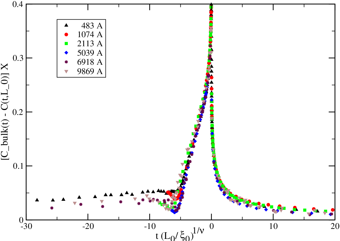
Note that $h^{\prime\prime}(0)\approx 3.05$ as can be obtained from the results of section 4.3 of [15]. For $x\gtrapprox-5$ the curves obtained from different thicknesses of the film fall reasonably well on top of each other. It has been noticed [11] that for $x\lessapprox-5$, in particular in the neighbourhood of the minimum, the results obtained for different thicknesses differ by quite large factors. In [15] we have computed the specific heat and the scaling function $f_{2}$ starting from the data for the energy density discussed above. We find that for $x\lessapprox-5$ our final result is clearly smaller than the experimental ones [16, 17].

Starting from the results for the finite size scaling function $h^{\prime\prime}(x)$ obtained from different thicknesses we have computed the scaling function $h^{\prime}(x)$. To this end, we have applied the trapezoidal rule. Similar to the previous section, we have started the integration at $x_{0}\approx 4$ in the high temperature phase. As starting value we have taken $h^{\prime}(x_{0})=\frac{x}{2\nu-1}h^{\prime\prime}(x_{0})$. Again we have integrated $h^{\prime}(x)$ using the trapezoidal rule to get $h(x)$. Here we have taken the same value for $x_{0}$ as above and $h(x_{0})=\frac{x}{2\nu}h^{\prime}(x_{0})$. Using these results for $h^{\prime}(x)$ and $h(x)$ we have computed $\theta(x)$ which we have plotted in figure 8.

In order to check the effect of errors due to the finite step-size of the integration, we have repeated the integration, skipping every second value of $x$. In order to check the effect of the singularity of $h^{\prime}(x)$ we have fitted the data for the specific heat in the neighbourhood of the transition with the ansatz

Then we have integrated the ansatz in the neighbourhood of the transition and compared it with the corresponding result from the trapezoidal rule. We find that the numerical results only change little and the conclusions drawn below are not effected.

Let us now discuss the results that we have obtained: For $483\AA$ the curve is monotonically decreasing with decreasing $x$; in particular no minimum of the function can be observed. For $1074\AA$ a shallow minimum occurs at $x\approx-5.3$; for $x\lessapprox 6.1$ the function is decreasing again with decreasing $x$. For $2113\AA$ we see a clear minimum at $x\approx-5.5$; However the value of the minimum is clearly smaller than the one of [20]. In the case of $5039\AA$ and $6918\AA$ we find a quite good match with our result [20] down to $x\approx-7$. For $6918\AA$ the minimum is located at $x\approx-4.8$ and the value of the minimum is $\theta\approx-1.3$. For $6918\AA$ the minimum occurs at $x\approx 4.65$ and the value of the minimum is $\theta\approx-1.36$. For $5039\AA$ no data for $x<-7$ are available. For $6918\AA$ the curve is decreasing again for $x\lessapprox-6.7$ with decreasing $x$. Up to here the expectation that with increasing thickness of the film the result converges toward the universal scaling function is fulfilled. However for the largest thicknesses studied, $9869\AA$ even the worst mismatch is found. The curve is monotonically decreasing with decreasing $x$ and even for $x\gtrapprox 5$ there is quite large mismatch with our result for $\theta$ [20]. Playing around with the data, one finds that smaller values of $h^{\prime\prime}(x)$ for $x\lessapprox-5$ are needed to avoid that $\theta$ is decreasing with decreasing $x$ for $x\lessapprox-5$. One should note that eq. (8) only holds for the scaling limit. Therefore the observations made here are not an indication that the experimental data are effected by an error. They can also be explained by corrections to the scaling behaviour. This is at least true for the smaller thicknesses like $483\AA$. The result for $9869\AA$ is more puzzling. One should note that the analysis presented in this section does not depend on the type of boundary conditions that is realized in the experiment. But we think that the behaviour of $\theta(x)$ for $x\lessapprox-5$ obtained here can not be explained by different boundary conditions from those used in the study of the lattice model [15, 20].

We have studied the relation of the excess specific heat, the excess energy and the thermodynamic Casimir force in thin films in the three-dimensional XY universality class. To this end we have exploited the relation (8)

among the finite size scaling functions $\theta(x)$ of the thermodynamic Casimir force, $h(x)$ of the excess free energy and $h^{\prime}(x)$ of the excess energy. We have analysed data obtained for the energy density of the improved two-component $\phi^{4}$ model on the simple cubic lattice and experimental results for the specific heat of thin films of ⁴He near the $\lambda$-transition [16, 17].

As a first exercise we have computed the functions $h^{\prime}(x)$ and $h(x)$ for a finite lattice of the size $L^{3}$ with periodic boundary conditions in all directions. This way we avoid potential problems related with the Kosterlitz-Thouless phase transition of the thin film and corrections caused by Dirichlet boundary conditions. Indeed we find a good collapse of the data already for rather small lattice sizes $L=8$, $16$ and $32$.

Next we have repeated the same exercise for films with free boundary conditions using the data for the excess energy density obtained in [15]. Here we find a huge mismatch between the thicknesses $L_{0}=8$, $16$ and $32$. Replacing $L_{0}$ by $L_{0,eff}=L_{0}+L_{s}$ with $L_{s}=1.02(7)$ [19] does not remove this discrepancy. We argue that the non-singular part of the energy density suffers from boundary corrections that are not described by the same $L_{s}$ which accounts for the corrections in singular quantities. Indeed, the analysis of the energy density of films up to the thickness $L_{0}=64$ at the critical temperature of the three dimensional system results in a $L_{sns}$ for the analytic background of the energy density that is clearly different from $L_{s}$. Taking into account this result we find a reasonable collapse of the functions obtained from $L_{0}=8$, $16$ and $32$ in a large range of the scaling variable $x$.

Computing the Casimir force from this result for $h^{\prime}(x)$ we find a good collapse for $-7\lessapprox x<4$. In this range of $x$ we also find a good agreement with the result for $\theta$ that we have obtained in [20]. Note that in particular the minimum of the scaling function $\theta$ is within this range. We confirm the position $x_{min}$ and the value $\theta_{min}$ that we have obtained in [20]. Next we took into account analytic corrects. The coefficients of these corrections were computed by matching the results obtained from $L_{0}=16$ and $L_{0}=32$. This way we could extend the range of agreement with our previous result [20] down to $x\approx-15$.

We have presented a viable alternative to compute the scaling function $\theta$ of the Casimir force. The nice agreement with our previous result [20] gives us further confidence in the correctness of the results.

Finally we have computed the scaling function $\theta$ using experimental results for the excess specific heat [16, 17]. Here we find a reasonable match with the theoretical results in the range $x\gtrapprox-5$. In particular we find evidence that the minimum of the scaling function $\theta$ is located at $x_{min}\approx 5$ which is consistent with our prediction [20] but slightly larger than $x_{min}=-5.45(12)$ [12] and $x_{min}=-5.7(5)$ [13], where the thermodynamic Casimir force has been determined for films of ⁴He with thicknesses $\lessapprox 600\AA$.

In the range $x\lessapprox-5$ the curves obtained from different thicknesses show quite different behaviour. Furthermore in this range $\theta(x)$ is decreasing with decreasing $x$. This behaviour corresponds to too large values of $h^{\prime\prime}(x)$ in the range $x\lessapprox-5$. We think that understanding this problem requires a detailed knowledge of the experiments and is therefore beyond the scope of the present work.

This work was supported by the DFG under the grant No HA 3150/2-1.

References

- [1] Fisher M E and de Gennes P-G, Phenomena at the walls in a critical binary mixture, 1978 CR Acad. Sci. Paris B 287 207
- [2] Gambassi A, The Casimir effect: From quantum to critical fluctuations , 2009 J. Phys. Conf. Series 161 012037
- [3] Campostrini M, Hasenbusch M, Pelissetto A, and Vicari E, Theoretical estimates of the critical exponents of the superfluid transition in 4He by lattice methods, 2006 Phys. Rev. B 74 144506 [cond-mat/0605083]
- [4] Wilson K G and Kogut J, The renormalization group and the -expansion, 1974 Phys. Rep. C 12 75
- [5] Fisher M E, The renormalization group in the theory of critical behavior, 1974 Rev. Mod. Phys. 46 597
- [6] Fisher M E, Renormalization group theory: Its basis and formulation in statistical physics, 1998 Rev. Mod. Phys. 70 653
- [7] Pelissetto A and Vicari E, Critical Phenomena and Renormalization-Group Theory, 2002 Phys. Rept. 368 549 [arXiv:cond-mat/0012164]
- [8] M. N. Barber Finite-size Scaling in Phase Transitions and Critical Phenomena, Vol. 8, eds. C. Domb and J. L. Lebowitz, (Academic Press, 1983)
- [9] Finite Size Scaling and Numerical Simulation of Statistical Systems, ed. V. Privman, (World Scientific, 1990).
- [10] Barmatz M, Hahn I, Lipa J A, and Duncan R V, Critical phenomena in microgravity: Past, present, and future, 2007 Rev. Mod. Phys. 79 1
- [11] Gasparini F M, Kimball M O, Mooney K P, and Diaz-Avila M, Finite-size scaling of 4He at the superfluid transition, 2008 Rev. Mod. Phys. 80 1009
- [12] Garcia R and Chan M H W, Critical Fluctuation-Induced Thinning of 4He Films near the Superfluid Transition, 1999 Phys. Rev. Lett. 83 1187
- [13] Ganshin A, Scheidemantel S, Garcia R, and Chan M H W, Critical Casimir Force in 4He Films: Confirmation of Finite-Size Scaling, 2006 Phys. Rev. Lett. 97 075301
- [14] Krech M, The Casimir Effect in Critical Systems (World Scientific, Singapore, 1994)
- [15] Hasenbusch M, The specific heat of thin films near the -transition: A Monte Carlo study of an improved three-dimensional lattice model, 2009 [arXiv:0904.1535]
- [16] Kimball M O, Mehta S and Gasparini F M, Superfluid Transition of 4He for Two-Dimensional Crossover, Heat Capacity, and Finite Size Scaling, 1999, J. Low Temp. Phys. 114 467
- [17] Kimball M O, Mehta S and Gasparini F M, Specific Heat Near the Superfluid Transition of a 0.9869 micron 4He Film, 2000, J. Low Temp. Phys. 121 29
- [18] Diehl H W, Dietrich S, and Eisenriegler E, Universality, irrelevant surface operators, and corrections to scaling in systems with free surfaces and defect planes, 1983 Phys. Rev. B 27 2937
- [19] Hasenbusch M, Kosterlitz-Thouless transition in thin films: A Monte Carlo study of three-dimensional lattice models, 2009 J. Stat. Mech. P02005 [arXiv:0811.2178]
- [20] Hasenbusch M, The thermodynamic Casimir effect in the neighbourhood of the lambda-transition: A Monte Carlo study of an improved three dimensional lattice model [arXiv:0905.2096]
- [21] Hucht A, Thermodynamic Casimir Effect in 4He Films near : Monte Carlo Results, 2007 Phys. Rev. Lett. 99 185301 [arXiv:0706.3458]
- [22] Vasilyev O, Gambassi A, Maciolek A, and Dietrich S, Universal scaling functions of critical Casimir forces obtained by Monte Carlo simulations, 2009 Phys. Rev. E 79 041142 [arXiv:0812.0750]
- [23] Campostrini M, Hasenbusch M, Pelissetto A, Rossi P, and Vicari E, Critical behavior of the three-dimensional XY universality class, 2001 Phys. Rev. B 63 214503 [cond-mat/0010360]
- [24] Hasenbusch M and Török T, High precision Monte Carlo study of the 3D XY-universality class, 1999 J. Phys. A 32 6361 [cond-mat/9904408]
- [25] Hasenbusch M, The three-dimensional XY universality class: A high precision Monte Carlo estimate of the universal amplitude ratio , 2006 J. Stat. Mech. P08019 [cond-mat/0607189]
- [26] Hasenbusch M, A Monte Carlo study of the three-dimensional XY universality class: Universal amplitude ratios, J. Stat. Mech. (2008) P12006 [arXiv:0810.2716]
- [27] Wolff U, Collective Monte Carlo Updating for Spin Systems, 1989 Phys. Rev. Lett. 62 361
- [28] Saito M, An Application of Finite Field: Design and Implementation of 128-bit Instruction-Based Fast Pseudorandom Number Generator, PhD thesis, Dept. of Math., Graduate School of Science, Hiroshima University, Advisor: M. Matsumoto; The numerical program and a detailed description can be found at “http://www.math.sci.hiroshima-u.ac.jp/˜m-mat/MT/SFMT/index.html”
- [29] Dohm V, 2008 Diversity of critical behaviour within a universality class, 2008 Phys. Rev. E 77 061128 [arXiv:0801.4096]
- [30] Newman K E and Riedel E K, Critical exponents by the scaling-field method: The isotropic N-vector model in three dimensions, 1984 Phys. Rev. B 30 6615
- [31] Kerr R C and Taylor R D, 1964, The molar volume and expansion coefficient of liquid 4He , Ann. Phys. 26 292
- [32]
The data are linked at the bottom of the page:
http://enthalpy.physics.buffalo.edu/Publications.html - [33] Lipa J A, Nissen J A, Stricker D A, Swanson D R and Chui T C P, Specific heat of liquid helium in zero gravity very near the -point, 2003 Phys. Rev. B 68 174518 [arXiv:cond-mat/0310163]
- [34] Lipa J A, Swanson D R, Nissen J A, Geng Z K, Williamson P R, Stricker D A, Chui T C P, Israelsson U E and Larson M, Specific Heat of Helium Confined to a 57-m Planar Geometry near the Lambda Point, 2000, Phys. Rev. Lett. 84 4894