Presentations of graph braid groups
Abstract.
Let be a graph. The (unlabeled) configuration space of points on is the space of -element subsets of . The -strand braid group of , denoted , is the fundamental group of .
This paper extends the methods and results of [11]. Here we compute presentations for , where is an arbitrary natural number and is an arbitrary finite connected graph. Particular attention is paid to the case , and many examples are given.
Key words and phrases:
graph braid group, configuration space, discrete Morse theory2000 Mathematics Subject Classification
Primary 20F65, 20F36; Secondary 57M15, 55R801. Introduction
Given a graph , the unlabeled configuration space of points on is the space of -element subsets of distinct points in . The -strand braid group of , denoted , is the fundamental group of .
Graph braid groups are of interest because of their connections with classical braid groups and right-angled Artin groups [7, 24, 12], and their connections with robotics and mechanical engineering. Graph braid groups can, for instance, model the motions of robots moving about a factory floor [16, 8, 9], or the motions of microscopic balls of liquid on a nano-scale electronic circuit [15].
Various properties of graph braid groups have been established. Ghrist showed in [16] that the spaces are s. Abrams [1] showed that graph braid groups are fundamental groups of locally CAT(0) cubical complexes, and so for instance have solvable word and conjugacy problems [3]. Crisp and Wiest [7] showed that any graph braid group embeds in some right-angled Artin group, so graph braid groups are linear, bi-orderable, and residually finite. For more information on what is known about graph braid groups, see for instance [23].
This paper continues a project begun in [11]. In [11], we used a discrete version of Morse theory (due to Forman [14]) to simplify the configuration spaces within their homotopy types. We were able to compute presentations for all braid groups , where is a tree; that is, for all tree braid groups ([11], Theorem 5.3). Our methods also allowed us, in principle, to compute a Morse presentation for any graph braid group.
Here we describe how to compute presentations for all graph braid groups , where is an arbitrary natural number and is a finite connected graph. As in [11], the generators in our presentations correspond to critical -cells, and the relators correspond to critical -cells. (In both cases, “critical” is meant in the sense of Morse theory.) Theorem 4.8 describes the general form of a relator in using “costs”, which are certain words in the group generators. Propositions 4.11 and 4.13 describe exactly how to compute these costs. Theorem 4.8 and Propositions 4.11 and 4.13 therefore completely describe presentations for all graph braid groups. The resulting presentations are particularly simple when . Note 5.3 describes a procedure for computing the relators in a 2-strand graph braid group, .
The paper is organized as follows. Section 2 contains a basic introduction to the version of discrete Morse theory that will be used in the rest of the paper. Section 3 describes a Morse matching on every ‘discretized’ configuration space . Section 4 shows how to use the ideas of the previous sections in order to compute presentations of graph braid groups. Section 5 collects some results about the case of two strands, and, in particular, contains the important Note 5.3 (as described above). Finally, Section 6 contains computations of presentations of , where or and is a balloon graph.
2. Background on Discrete Morse Theory
2.1. A motivating example
Example 2.1.
Consider the ‘star’ tree , – the tree with exactly vertex of degree and vertices of degree . Then is a free group of rank (cf. [16, 6]). Ghrist described the entire configuration space as a union of squares and triangles. The configuration space is reproduced here on the left in Figure 1. The three (distorted) squares correspond to configurations in which the two strands occupy different branches of . There are three squares since there are three ways of choosing two edges from a set of three. The triangular flaps are copies of the configuration space , where is the unit interval. These flaps correspond to configurations in which both strands occupy the same closed edge.
Adjacent to our reproduction of Ghrist’s is a space homeomorphic to , where the central missing point has been expanded into a triangle. We use this picture to show the configuration spaces where .
We begin with . It is straightforward to see that we need to assemble the configuration space out of copies of , for a total of squares (the number of ways of choosing edges for the two strands) and triangles (the number of ways of choosing edge for both strands). In , the squares and triangles were joined together along a common edge, with cross-section a copy of . In , the squares and triangles will also come together along a common edge, but with as cross-section. It is also straightforward to see that the desired shape for should resemble the -skeleton of the -simplex. Indeed, as deformation retracts onto the -skeleton of the -simplex (that is, a triangle), so deformation retracts onto the -skeleton of the -simplex.
These arguments generalize as follows. We build the configuration space from the -skeleton of a -simplex. For each vertex of the simplex, has a half-open edge (that is, one endpoint is present and one is not), labeled . For each -cell of the simplex, has a square which is closed except that it is missing a single corner. A square is attached to the edges and corresponding to the endpoints and of , along adjacent faces of , so that the missing endpoints of and match the missing corner of . Finally, to each edge of there is attached a right triangle, which is closed except that it is missing a single corner adjacent to the hypotenuse. The triangle is glued to along the side from the right angle to the missing corner, so that the missing corner lines up with the missing vertex of .
The deformation retraction onto the -skeleton of the -simplex is then clear, reinforcing the calculation that is a free group of rank .
Even for very simple graphs like the graphs , the full configuration space can quickly contain much more information than is necessary to understand the behavior of the corresponding graph braid group. As this example shows, there is a lot of extraneous information contained in the full configuration space, and the configuration spaces can quickly become difficult to visualize. There are much smaller homotopy equivalent spaces, like the -skeleta of simplices indicated here, which carry all of the homotopy data needed to compute presentations of the graph braid groups. Indeed, even the -skeleta of simplices, although -dimensional instead of -dimensional, are still too large and themselves have the homotopy types of bouquets of circles.
As in this example, we wish to simplify configuration spaces of graphs down to smaller, more manageable spaces. We use Forman’s discrete Morse theory to formalize a method of simplifying these configuration spaces. Discrete Morse theory deals with CW complexes, but as we will see in Section 3, this is not a problem for us.
2.2. Discrete Morse theory: definitions
In this subsection, we collect some basic definitions (including the definition of a Morse matching) from [11] (see also [4] and [14], which were the original sources for these ideas).
Let be a finite regular CW complex. Let denote the set of open cells of . Let be the set of open -cells of . For open cells and in , we write if and , where is the closure of , and if or .
A partial function from a set to a set is a function defined on a subset of , and having as its target. A discrete vector field on is a sequence of partial functions such that:
- (1)
Each is injective;
- (2)
if , then ;
- (3)
.
Let be a discrete vector field on . A -path of dimension is a sequence of -cells such that if is undefined, then ; otherwise and . The -path is closed if , and non-stationary if . A discrete vector field is a Morse matching if has no non-stationary closed paths.
If is a Morse matching, then a cell is redundant if it is in the domain of , collapsible if it is in the image of , and critical otherwise. Note that any two of these categories are mutually exclusive by condition (3) in the definition of discrete vector field.
The ideas “discrete Morse function” and “Morse matching” are largely equivalent, in a sense that is made precise in [14], pg. 131. In practice, we will always use Morse matchings instead of discrete Morse functions in this paper (as we also did in [11]). A Morse matching is sometimes referred to as a “discrete gradient vector field” in the literature; in particular, we used this more cumbersome terminology in [11].
2.3. Discrete Morse theory and fundamental group
Section 2 of [11] described how to compute the fundamental group of a finite regular CW complex using a Morse matching defined on . This is done as follows.
Choose an orientation for -cells in , and let denote the set of all oriented -cells and their inverses, treated as an alphabet. For every -cell in , we want to rewrite the -cell in terms of -cells that are critical under . Consider a word in . For any words , , and in and any single oriented -cell , we define the following moves:
- (1)
(free cancellation) If or , write .
- (2)
(collapsing) If and is a collapsible -cell, write .
- (3)
(simple homotopy) If or , and is a boundary word for a -cell satisfying , write or , respectively.
Let denote the reflexive transitive closure of , as in [11].
Proposition 2.4 of [11] implies that any sequence
must terminate in a reduced word, i.e., one that is not the source of any arrow. Furthermore, this reduced word is uniquely determined by , not the particular sequence of arrows. We denote this reduced word . The free cancellation property shows is freely reduced, and the collapsing and simple homotopy properties guarantee consists entirely of critical -cells.
Theorem 2.2.
([11]) Let be a finite regular connected CW complex and let be a Morse matching with only one critical -cell. Then:
where is the set of positively-oriented critical -cells, and is the set of all words in , where runs over all boundaries of critical -cells.
Proof.
This theorem is almost exactly Theorem 2.5 of [11], with the simplifying assumption that there is only critical -cell. Under this assumption, Propositions 2.2(2) and 2.3(5) of [11] imply that the union of all collapsible edges is a maximal tree in . Thus, the tree named in Theorem 2.5 of [11] contains no critical -cells. The statement of the theorem given here then follows. ∎
3. Morse Matchings for Configuration Spaces of Graphs
3.1. The complex
The configuration spaces were used to define graph braid groups, but unfortunately these have no natural CW-complex structure. We need slightly different spaces, which we describe here.
Let be a finite connected graph and a natural number. Let denote the union of those open cells of (equipped with the product cell structure) whose closures intersect the fat diagonal . Let denote the space , called the discretized configuration space of points on . Note that inherits a CW complex structure from the Cartesian product. A cell in has the form such that: each is either a vertex or the interior of an edge, and the closures of the are mutually disjoint.
Let denote the quotient of by the action of the symmetric group which permutes the coordinates. Thus, an open cell in has the form such that: each is either a vertex or the interior of an edge, and the closures are mutually disjoint. The set notation is used to indicate that order does not matter.
Under most circumstances, the labeled or unlabeled configuration space of is homotopy equivalent to the corresponding discretized version. Specifically:
Theorem 3.1.
[19, 1, 22] For any integer and any graph with at least vertices, the labeled (unlabeled) configuration space of points on strong deformation retracts onto () if
- (1)
each path between distinct vertices of degree not equal to passes through at least edges; and
- (2)
each path from a vertex to itself which is not null-homotopic in passes through at least edges.
This theorem was orignally proved by Hu [19] for the case . Arbitrary was done by Abrams [1], but with a slightly weaker first condition. Full generality is proven by Prue and Scrimshaw [22], who also address a minor flaw in the proof of Abrams.
A graph satisfying the conditions of this theorem for a given is called sufficiently subdivided for this . It is clear that, for any fixed , every graph is homeomorphic to a sufficiently subdivided graph.
Throughout the rest of the paper, we work exclusively with the space where is sufficiently subdivided for . Also from now on, “edge” and “cell” will refer to closed objects.
3.2. Some definitions related to the Morse matchings
This section contains definitions which will help us when we define Morse matchings on the complexes in Subsection 3.3.
As usual, let be a finite connected graph. For a vertex of , let or just denote the degree of . If , then is called an essential vertex.
We define an order on the vertices of as follows. Choose a maximal tree in . Edges outside of are called deleted edges. Pick a vertex of degree in to be the root of . Choose an embedding of the tree into the plane. Begin at the basepoint and walk along the tree, following the leftmost branch at any given intersection, and consecutively number the vertices by the order in which they are first encountered. When a vertex of degree one is reached, turn around. The vertex adjacent to is assigned the number , and is (in effect) numbered . Note that this numbering depends only on the choice of and the embedding of the tree. For two vertices and , we write if receives a smaller number than (i.e., if is encountered before in a clockwise traversal of from ). We let denote the open interval in the order on vertices:
When we write , we mean the geodesic connecting to within . The meet of two vertices and in , denoted is the greatest vertex in the intersection .
For a given edge of , let and denote the endpoints of . We orient each edge to go from to , and so that . Thus, if , the geodesic segment in must pass through . For a vertex , let be the unique edge in satisfying .
The choice and embedding of allow us to refer to directions in , as follows. If is a vertex in the tree , we say that two vertices and lie in the same direction from if the geodesics start with the same edge. Thus, there are directions from a vertex . We number these directions , beginning with the direction represented by , numbered , and proceeding in clockwise order. A vertex is considered to be in direction from itself. We let denote the direction from to (which is an integer). When referring to a direction from a vertex to an edge, we are referring to the direction from the given vertex to the initial vertex of the edge.
To define the Morse matching on , we will need the following definitions. Let be a cell in . A vertex in is blocked in if either or for some other vertex or edge of aside from ; we say is blocked by or in , respectively. If is not blocked in , it is called unblocked in . Equivalently, is unblocked in if and only if is also a cell in .
An edge in is called non-order-respecting in if:
- (1)
, or
- (2)
there is some vertex of such that and .
An edge in is order-respecting in otherwise.
3.3. The Morse matching
In this subsection, we will define a Morse matching on for an arbitrary positive integer and finite connected graph .
Suppose that we are given a cell in . Assign each cell in a number as follows. A vertex of is given the number from the above traversal of . An edge of is given the number for . Arrange the cells of in a sequence , from the least- to the greatest-numbered. The following definition of a Morse matching is equivalent to the definition of from [11], by Theorem 3.6 of the same paper.
Definition 3.2.
We define a Morse matching on as follows:
- (1)
If an unblocked vertex occurs in before all of the order-respecting edges in (if any), then is obtained from by replacing the minimal unblocked vertex with . In particular, is redundant.
- (2)
If an order-respecting edge occurs in before all of the unblocked vertices of (if any), then , i.e., is collapsible. The cell is obtained from by replacing the minimal order-respecting edge with .
- (3)
If there are neither unblocked vertices nor order-respecting edges in , then is critical.
Example 3.3.
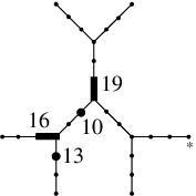
Figure 2 depicts three different cells of for the given tree . In each case, the number label of each vertex and of the initial vertex of each edge are shown, in the sense mentioned above.

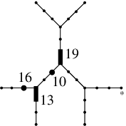
We let denote the cell depicted in (a). The vertex numbered is blocked. The vertex numbered is unblocked, so is redundant. Note that edge is order-respecting and edge is non-order-respecting. We get by replacing vertex with the unique edge in having vertex as its initial vertex, i.e., .
Let denote the cell depicted in (b). The vertex numbered in is blocked. The edge is order-respecting, so is collapsible. Note that vertex is blocked and edge is non-order-respecting. The description of above implies that is obtained from by replacing edge with its initial vertex.
The cell depicted in (c) is critical since vertices and are both blocked, and the edges and are non-order-respecting.
4. Presentations for Graph Braid Groups
4.1. Preliminary notation
In this subsection, we include some final notation before we proceed to the main argument.
We will sometimes use set notation in order to describe edge-paths. For instance, suppose that is the tree from Figure 2. The edge-path starts at the vertex and ends at . The edges of this edge-path are determined by moving the vertex whose original position is back to the basepoint . (There are edges in all.) All of the other vertices are fixed.
Let be a -cell in . If has no unblocked vertices, define . Otherwise, if is the smallest unblocked vertex in , define to be the -cell that may be obtained from by replacing with (i.e., the vertex adjacent to along the edge-path , where is the maximal tree). For instance, if where (as in Figure 2), then . We let denote the result of repeatedly applying to until the output stabilizes (as it obviously must).
We will frequently need to describe cells in using vector notation, as was done in [11]. Let be an essential vertex in , the maximal subtree of . We let be a vector with entries, all of which are non-negative integers. Let , and let denote the th coordinate of , for . We write do denote the sum of entries of . By , we denote a configuration (or subconfiguration) of vertices and edges such that:
- (1)
There is an edge such that , and points in direction from . There are vertices blocked by ;
- (2)
For each , there are vertices lying in direction from , and blocked by the edge .
Note that if , then . When we use this vector notation, we typically assign each essential vertex in a capital letter of the alphabet, in alphabetical order.
For instance, suppose that is as in Figure 2. We write in place of , in place of , and so on. We can also use additive notation to describe higher-dimensional cells. For instance, the critical -cell depicted in Figure 2(c) can be described by the notation . The collapsible -cell in Figure 2(b) can be described as .
We will also occasionally extend this additive notation to describe cells containing deleted edges and vertices blocked at the basepoint. Thus, for instance, we might write to denote a cell consisting of the configuration along with the deleted edges and , and vertices blocked at the basepoint. In practice, we will typically leave off when describing a cell in , since this should cause no confusion.
It is easy to deduce under fairly general assumptions (for instance, see Assumption 4.10) that a formal sum consisting of terms of the form (where is an essential vertex), and others of the form (where is a deleted edge), is critical if and only if each term of the form satisfies , for some . (Note: we also assume of course that is a vector with non-negative integer entries, and that .) Indeed, the critical cells of are in one-to-one correspondence with such formal sums. (A more explicit version of this statement appears as Proposition 3.9 of [11].)
We need some final definitions for technical reasons. We multiply vectors by constants in the obvious way. We also define subtraction of a constant from a vector, as follows. Let be the result of subtracting from the first non-zero entry of . We let , and so on. We note that this notation must be used with caution, since in general. Finally, we let denote the vector such that and , for all . The number of components of will always be clear from the context.
4.2. Relative flow, cost, and the main theorem
We now give some examples, which are intended to the smooth the way for our proofs of Theorem 4.8, Proposition 4.11, and Proposition 4.13. The following example is intended, above all, to motivate Definition 4.4.

Example 4.1.
We let be the graph depicted in Figure 3, and consider the two-strand braid group of . Let denote the maximal tree in consisting of all edges and vertices of ,except for the dashed edges in Figure 3. The figure also indicates a choice of embedding of in , a choice of basepoint in , and the resulting numbering of the vertices of .
It is a simple matter to list the critical -cells and -cells. The critical -cells are as follows:
There is a single critical -cell:
It follows from Theorem 2.2 that has a presentation with five generators and one relator.

Now we will find the relator in this presentation. The critical -cell can be identified with the product . If we recall that is the initial vertex of and is the initial vertex of (and we treat the factor of as the first factor), then we arrive at the central oriented square in Figure 4. The bottom left vertex of this square is , the upper left corner is , the upper right corner is , and the lower right corner is .
Consider the bottom horizontal face of the critical -cell . This is the -cell . Clearly this -cell is redundant; its image under the Morse matching is (as pictured in Figure 4; this cell is immediately below ). The Morse matching therefore tells us to push the -cell across the -cell . In the process, is smeared across the edge-path
which makes up the sides and bottom of the -cell . We repeat this procedure two more times, pushing across , and finally pushing across . The cumulative effect is to smear the original -cell across the edge-path
| (P1) |
Note that we haven’t yet completed the process of pushing redundant -cells across their matching collapsible -cells, since , , , and are all redundant -cells. We will finish after introducing a lemma (Lemma 4.2 below). For now, we note that Figure 4 shows that the Morse matching smears the left, top, and right sides of the critical -cell across the edge-paths
| (P2) | ||||
| (P3) | ||||
| (P4) |
respectively.
Lemma 4.2.
(Redundant -cells lemma) Assume is a redundant -cell in . We assume that the vertex is the smallest unblocked vertex in . Assume that is the maximal tree in .
- (1)
If , then .
- (2)
If and , then .
Proof.
Example 4.3.
We apply the previous lemma to the edge paths from the end of Example 4.1. Edge-path (P1) contains the subpath , which is made up of the edges , , and . The first and last of these edges flow to the trivial word by Lemma 4.2(2). The remaining edge, , flows to by Lemma 4.2(1). The edge is critical, and therefore stable under the flow. We can apply the flow to the subpath just as we did to the subpath . The result is that flows to . We conclude that (P1) flows to
Similarly, the edge-paths (P2), (P3), and (P4) flow, respectively, to:
If we rename the critical -cells , , , , and as , , , , and (respectively), then
by Theorem 2.2. It is easy to rewrite this presentation to show that , where is the free group on three generators.
Definition 4.4.
(Relative Flow) Let be a collection of vertices, and let be a closed edge in . We assume that is non-order-respecting in . We define an edge-path inductively as follows. If all vertices in are blocked, then is the trivial path at . Otherwise, let be the smallest unblocked vertex in the configuration . Without loss of generality, . We set . By definition,
The latter equation completely determines . We can define analogously: simply replace with in the above notation (while leaving the definition of unchanged).
The edge-path is called the flow of relative to . We write . The string is a word in the free group on critical -cells called the cost of relative to .
Note 4.5.
If is a collection of vertices and is a non-order-respecting edge in the configuration , then the relative flow is an edge-path in with a simple direct description. We start with the vertex in and repeatedly move the vertices of while following these rules:
- (1)
The vertex never moves.
- (2)
At each stage, we move the smallest unblocked vertex one step within the tree towards the basepoint . Here a vertex is considered blocked (for the sake of this definition) if the vertex is blocked in the ordinary sense by .
Note 4.6.
Although the notation features a vertex () in the second place, we need to keep track of both an edge () and an endpoint (, in this case). We write for the sake of compression. It would be ambiguous to specify only a vertex, since the edge is allowed to block the movements of vertices. Nevertheless, we will sometimes write (i.e., specify only a vertex in the second coordinate) if the edge in the definition of the relative flow never blocks the movements of any vertices, or if the identity of the edge is clear from the context.
Example 4.7.
Consider the tree in Figure 5. Let . The given is sufficiently subdivided for . We let and , and consider the relative flow . We have
Thus, is an edge-path of length .
The cost is obtained by applying the flow to . It is clear in this case that , since Lemma 4.2(2) applies to each of the six -cells in .

Theorem 4.8.
(General Presentation Theorem) Let be a finite connected graph. Let . Assume that is sufficiently subdivided for . The braid group has a presentation where is the set of critical -cells in , and is in one-to-one correspondence with the set of critical -cells in . A critical -cell corresponds to the relator in Figure 6, where .
Proof.
We need only show that the critical -cell corresponds to the relator appearing in Figure 6; the rest of the statement is a corollary of Theorem 2.2.
Let us consider the -cell . We wish to show that
| (*) |
(The right side of the latter equation labels the left arm of the plus sign in Figure 6.) We begin by noting that cannot be collapsible. Indeed, since is critical, it must be that is non-order-respecting, so either i) is not contained in the maximal tree , or ii) , and there is a vertex such that , and . Moreover, both of these conditions are inherited by .
It follows that is either critical or redundant. We assume first that is critical. In this case, each vertex in is blocked, so, by definition, and are both trivial paths, , and . It follows that (* ‣ 4.2) is satisfied in the current case.
Now suppose that is redundant, and so has an unblocked vertex. We write , and let denote the smallest of all unblocked vertices in . (We note that could be , i.e., .) We let
By definition
Now we apply to both sides. By induction, we have that is equal to
Finally, we note that
Condition (* ‣ 4.2) follows directly. One applies the same reasoning to each of the three remaining faces of . ∎
Example 4.9.
We let be the tree from Figure 2, and let . It is possible to show that the space has critical -cells and critical -cells. We will compute the relator corresponding to the critical -cell .
We compute each of the eight costs.
- (1)
- (2)
The flow is equal to (but with in place of ), so . The costs , , , and are trivial also, since the corresponding flows are again made up of edges satisfying the hypotheses of Lemma 4.2(2).
- (3)
We compute the relative flow :
All of the edges in this edge-path satisfy the hypotheses of Lemma 4.2(2), with the exception of . If we apply Lemma 4.2(1) to the latter edge repeatedly, we eventually conclude that
Since all of the other edges in flow to , we have . Exactly the same argument shows that .
4.3. Calculation of costs
In the previous example, at least one of the costs at any corner of a given critical -cell was trivial. This is true under fairly general hypotheses.
Assumption 4.10.
Let . Assume that is subdivided and the maximal tree is chosen in such a way that:
- (1)
Each vertex of degree in has degree at most in , and
- (2)
is sufficiently subdivided for .
Proposition 4.11.
(Vanishing Costs) Assume that and satisfy Assumption 4.10 for . Let be a critical -cell in . Let . One of the costs , is trivial. More specifically, in all of the following cases.
- (1)
, and
- (a)
, or
- (b)
.
- (a)
- (2)
, and .
- (3)
, , and
- (a)
, or
- (b)
.
- (a)
- (4)
, , and there is some vertex such that .
Proof.
We first assume that , . In this case, since all vertices in are blocked, each vertex is either blocked by , blocked by , or blocked at the basepoint. (Here we mean that a vertex is blocked by if is either blocked by in the usual sense, or that is blocked by a vertex that is blocked by , etc.)
Assume that . We note first that the vertex and each vertex blocked by will eventually be blocked by after it has moved (possibly several times) by our assumption. It follows that the relative flow is the edge-path determined by moving each of the vertices blocked at and in order, until all are blocked at . Each edge in this edge-path has the property that . It follows that , and so , as claimed.
Assume now that . In this case, the vertex and each of the vertices blocked by will eventually be blocked at the basepoint after moving several times. The relative flow is the edge-path determined by moving and each of the vertices blocked by in order until all are blocked at the basepoint. Each edge in this edge-path has the property that (as before). (Indeed, each edge must in fact be collapsible, in contrast with the situation covered in the previous case.) It follows again that . This proves (1).
Now we assume that , and . Since is critical. Because and satisfy Assumption 4.10, it must be that all of the vertices are blocked at the basepoint . The relative flow is the edge-path obtained by starting at the vertex and repeatedly moving the vertex until it is blocked at the basepoint. All of the edges in this path are collapsible, so . This proves (2).
Now assume that and . Assume also that , as in (3a). In this case, the vertex consists of a collection of vertices blocked by , a (possibly empty) collection of vertices blocked at , and the vertices and . The assumption implies that will eventually be blocked by (possibly after moving several times). As is the only unblocked vertex, the relative flow is the edge-path starting at which is determined by repeatedly moving until it is blocked by . Each edge in this edge-path is collapsible, so .
Assume that , , and , as in (3b). In this case, all of the vertices are either blocked by , or blocked at the basepoint. Since , the vertex can be moved repeatedly until it is blocked at the basepoint. The relative flow is the edge-path beginning at which can be obtained by moving repeatedly until it is blocked at the basepoint. All of the edges in this path are collapsible, so . This prove (3).
Finally, we consider case (4): , , and there is some vertex such that . The vertices are all either blocked by , or blocked at . It follows from our assumptions that each vertex in is less than , so consists entirely of collapsible edges. Therefore , proving (4).
The main statement, that one of or is trivial, follows, because if fails to satisfy any of the conditions (1)-(4), then it must satisfy one of the conditions (1’)-(4’), where (1’)-(4’) are the conditions that are be obtained from (1)-(4) by reversing the roles of and (and of and ). ∎
Note 4.12.
In Proposition 4.13, certain of the costs, which are necessarily words in the alphabet of oriented critical -cells, are described using both collapsible and critical -cells. This is a slight abuse of notation. In the event that a cost contains collapsible -cells among its letters, then one should apply the collapsing rule from Subsection 2.3 to remove each such -cell from the final form of the cost.
Proposition 4.13.
(Costs ) Assume that is a critical -cell. We frequently write in place of . Let . Let and , and let be the direction from along and the direction from along .
- (1)
Assume .
- (a)
If , then
- (b)
If , then
where , , and .
- (c)
If , then
- (a)
- (2)
Assume . Then has the form .
- (a)
If , then
Here is the place of the first non-zero coordinate in (in the first case) or in (in the second case).
- (b)
If (where ), and , then
- (c)
If or if and , then
- (a)
- (3)
Assume and . Then has the form .
- (a)
If and , then
- (b)
If or , then
- (a)
- (4)
Assume and . Then has the form .
- (a)
If , then
Here again is the place of the first non-zero coordinate in (in the first case) or in (in the second case).
- (b)
If and , then
- (c)
If and , then
- (a)
Proof.
- (1)
Subcase (a) is covered by Proposition 4.11. For Subcase (b), we assume first that and that neither nor contains the basepoint . It follows that . The flow is therefore simply the edge-path . The edge-path (in ) contains a unique edge such that . The only edge in contributing to is therefore , as all other edges in satisfy the hypotheses of Lemma 4.2(2). We note that . Now we apply the flow to ; since and all other vertices are blocked, we may apply Lemma 4.2(1) repeatedly, moving until it is blocked by . The resulting cell is clearly , and therefore , as claimed.
The proof is essentially the same if one of and contain the basepoint. We omit the argument.
Finally, for Subcase (c), we assume . Then , which is made up entirely of collapsible edges. Therefore in this case as well.
- (2)
We first consider the cost in Subcase (a). The flow has the initial vertex . The elements of this vertex (all of which are vertices in ) are of two types. First, there are vertices blocked by , and itself. Second, there are vertices clustered around the essential vertex , where the number of such vertices in the direction from is the th component of . The flow is determined by successively moving each of the latter vertices back to the basepoint, beginning with the smallest-numbered.
We suppose, without loss of generality, that is the smallest of the vertices clustered at . Note that is the edge pointing in direction from . The edge-path must consist entirely of collapsible edges, except possibly the first edge , by Lemma 4.2(2). We assume for the moment that is not collapsible. It follows that there are vertices of contained in the interval . The only possibility is that the set of all such vertices is precisely the set of vertices clustered around . If we apply the flow to the edge , we therefore arrive at the cell
(1) This cell is critical under our current assumptions (i.e., that is not collapsible), because we must have . If is collapsible, then we must have . This implies that (1) is trivial. It follows therefore that is equal to (1) in any case. This is the first factor in the cost.
We now continue, moving the second vertex from the cluster at . We can apply the same reasoning as before, but this time we replace the vector in the above reasoning with . It follows that the second factor in the cost is
where is as defined in the theorem. (We note that depends on .) One repeats this reasoning, eventually arriving at the formula in the statement of the theorem.
We now consider the cost . The computation of this cost is exactly like that of , except that the smallest vertex can always be moved freely to the basepoint, contributing nothing to the cost, since is smaller than all of the vertices clustered around (and ). This leaves us to repeat the calculation of the previous paragraphs, but beginning with rather than . This establishes the desired identity.
We now consider Subcase (b). Since and , it follows that . The initial vertex of the flow consists of vertices clustered around and vertices clustered around . The flow is the edge-path determined by moving the vertices at back to the basepoint, while holding those at fixed.
We let be the smallest of the vertices clustered at . We move back to the basepoint . All of the edges along the resulting edge-path (in ) are collapsible, contributing nothing to the cost, with the sole exception of , where is the edge pointing in direction from . Now we repeatedly apply Lemma 4.2(1) to , to arrive at
(2) This is the first factor in . Now we repeat this argument, replacing with in the above reasoning. We eventually arrive at the cost in the statement of the Theorem.
- (3)
The cost in (3a) is essentially identical to the cost in (2b) (simply replace with ), and it is computed in essentially the same way. Subcase (3b) follows from Proposition 4.11(3).
- (4)
The formulas for cost in (4a) and (4b) are the same as those in (2a) and (2b) (respectively) if we let , and they are proved in a directly analogous way. Subcase (4c) follows from Proposition 4.11(4).
∎
5. The Case of Two Strands
We let , and continue to assume that and satisfy Assumption 4.10. This means simply that is a simplicial graph, and that is a maximal tree in such that each vertex having degree in has degree at most in . We begin by describing the costs .
Proposition 5.1.
(Costs in the case ) Let and assume that , satisfy Assumption 4.10. Assume that and are endpoints of deleted edges. We let , and let and .
- (1)
If or if , then .
- (2)
If and , then .

Example 5.2.
We let , let be the graph pictured in Figure 7, and let be the indicated maximal tree.
There is just one critical -cell, . Now note that , , and all other costs are trivial. (Here we’ve written rather than for the sake of brevity.) If we let and , then
It is clear therefore that is a free group on three generators.
Note 5.3.
Theorem 4.8 and Proposition 5.1 together give a general method for finding the relation corresponding to a given critical -cell in the case (and, therefore, for finding presentations for the groups ). The method can be sketched as follows. We suppose that and let denote the critical -cell consisting of the edge and a single vertex blocked at the basepoint. (That is, if , and otherwise.)
- (1)
We begin by drawing an octagon and labelling four of the faces (as pictured below).

Figure 8. The relators in a presentation for can be represented by labelled octagons. Here is one such octagon, with four of the eight sides labelled. - (2)
Each of the four remaining faces will be labelled by a single critical -cell (or by the trivial element). This follows from Proposition 5.1 and Theorem 4.8. We now determine the orientations on each of the slanted faces. Consider first the orientation on the bottom left slanted face. If , then the orientation on the bottom left face points up and to the left; if , then the orientation points down and to the right. Thus, if , then the orientation points from the initial vertex of to the initial vertex of .
One follows exactly the same procedure at each slanted face: the orientation points away from the larger vertex, and towards the smaller vertex (if we confuse, for the moment, the edges and ()).
- (3)
Finally, we label each corner with a critical -cell (i.e., a generator). Consider the bottom right corner, which connects the terminal vertex of with the initial vertex of . Let denote . Let and . If either or , which can happen only if or (respectively), then we label the corner with . Otherwise, we label the corner with either (if it is critical) or with (if it is critical). (Exactly one of these cells is critical, and the other is collapsible.)
Example 5.4.
Consider , where is the graph depicted in Figure 9. We have chosen a subdivision of and an embedding of into the plane.


We follow our usual convention for labelling essential vertices by letters (see Subsection 4.1), so , , , , and . There are eleven critical -cells: (), , , , , and , for . There are six critical -cells ().
We can follow the procedure sketched in Note 5.3 in order to find the relations. They are pictured in Figure 10.
We can eliminate by Tietze transformations the generators , , , , , and (in that order). The resulting presentation shows that is a free group on five generators:
Proposition 5.5.
If is a graph such that there exists a vertex in which is on every simple loop in , then is free.
Proof.
We want to show that one can choose a maximal tree such that every deleted edge touches . Since critical -cells in are in one-to-one correspondence with unordered pairs of disjoint deleted edges, the existence of such a tree shows that there are no critical -cells, and therefore that the Morse presentation of defines a free group.
We now find a tree with the desired property. The assumptions imply that consists of a disjoint union of trees . We fix a tree . Certain of the edges of are half-open, since their closures contain . We let denote these half-open edges. We let
where denotes the interior of . Note that contains , and so is a tree with exactly 1 leaf at . The union is thus a maximal tree in with the property that all edges touch . ∎
Theorem 5.6.
Let be a graph in which every pair of simple loops is disjoint. The group has a Morse presentation such that all relators are commutators corresponding to pairs of simple loops.
Proof.
We consider a copy of (with maximal tree ) satisfying Assumption 4.10. Let be a critical -cell in . It follows that for some deleted edges .
We first note that is a simple loop for , so, in particular, . We let denote the smallest vertex on for . We assume, without loss of generality, that .
The relation determined by takes the following form, by Theorem 4.8:
| (3) |
where
| (4) |
for . It will follow that the above relation is a commutator relation if we show that and may both be replaced by in all of the above costs, for then and , so the above relation becomes
We first show that . There are two cases: either or . If , then all of the vertices on are greater than all of the vertices on . The flows and both contain the subpath . This subpath contains the only edge making a contribution to either cost, namely , where is the edge pointing in direction from . Therefore, . If , then the argument is similar, except that the only contribution comes from the edge , where is the edge pointing in direction from . The edge is still common to the edge-paths and , and therefore .
Now we show that . If (and therefore and ), then all of these costs are trivial, so we may assume that . Now the path doesn’t contain the point , so there will be a unique edge in the edge-path such that .
We claim that . Indeed, the inequality implies that . It is clear that , so . It follows directly that . The inequalities follow from the definition of . This proves the claim.
The flows and contain the edges and (respectively; as above), and these are the only edges that will contribute to the costs. Both of these edges flow to by Lemma 4.2(1), where is the vertex adjacent to satisfying . It follows that .
The preceding argument shows that and may be replaced by in the costs , , , and . Essentially the same argument show that and may be replaced by in the costs involving (rather than ).
To finish the proof, we note that unordered pairs of disjoint simple loops are in bijective correspondence with unordered pairs of distinct deleted edges; i.e., with critical -cells, and therefore with relators in the Morse presentation. ∎
The following conjecture is a large generalization of Theorem 5.6:
Conjecture 5.7.
Let be a planar graph. Then there exists a presentation for such that the relators are all commutators corresponding to pairs of disjoint simple loops.
An original goal for this paper was to prove this conjecture. In a large number of examples, the authors have verified the result. In general, though, a proof is elusive.
6. A Class of Examples
Let . The wedge sum of with the circle along the basepoint is called a balloon. A balloon graph is a wedge sum of a finite collection of balloons with a line segment, where all basepoints in the wedge sum are of degree one. A balloon graph is uniquely determined up to homeomorphism by the number of its balloons.
Fix a balloon graph with balloons. We will compute presentations of for .
6.1. The case

We will let denote the lower essential vertex of degree . We will let denote the th vertex of degree three from the left (so is part of the circle containing the edge ).
The critical -cells in are of three types:
- (1)
There are critical -cells , where . We let denote the critical -cell .
- (2)
A total of critical -cells are described by the vector notation (). Since a critical -cell of this type is completely determined by the essential vertex , we write in place of .
- (3)
A total of critical -cells are described by the vector notation (). We denote these .
There are critical -cells, all of the form (). It is straightforward to follow the procedure from Note 5.3 and arrive at the following relations.
This gives us the following presentation for :
6.2. The case
We choose a version of satisfying the Assumption 4.10. We carry over our convention of labelling essential vertices from the case .
The critical -cells in are of three types:
- (1)
There are critical -cells , where . We let denote the critical -cell .
- (2)
A total of critical -cells are described by the vector notation (; ). A critical -cell of this type is completely determined by , , and , so we write instead.
- (3)
A total of critical -cells are determined by the vector notation (; ; ). An additional critical -cells are determined by (; ). This makes a total of critical -cells of this type.
We therefore have a total of critical -cells.
There are two types of critical -cells:
- (1)
There are critical -cells of the form ().
- (2)
We can form the other critical -cells by making a choice of a deleted edge () and a choice of a critical subconfiguration ) or (). This makes possible critical -cells of this kind.
It follows that there are critical -cells in all.
The relators take several different forms. We simply enumerate the possible cases, describe the relators, and leave the verifications to the interested reader.
- (1)
(): The relator is:
- (2)
():
- (3)
():
- (4)
():
- (5)
():
- (6)
():
- (7)
():
- (8)
():
- (9)
():
Finally, we notice that all of the above relators are commutators, with the exception of those from (2). We can eliminate each of the latter relations by Tietze transformations, and (at the same time) eliminate the generators (). The resulting presentation for has generators and relators, all of which are commutators.
References
- [1] Aaron Abrams. Configuration spaces of braid groups of graphs. PhD thesis, UC Berkeley, 2000.
- [2] Aaron Abrams and Robert Ghrist. Finding topology in a factory: configuration spaces. Amer. Math. Monthly, 109(2):140–150, 2002.
- [3] Martin R. Bridson and André Haefliger. Metric spaces of non-positive curvature, volume 319 of Grundlehren der Mathematischen Wissenschaften [Fundamental Principles of Mathematical Sciences]. Springer-Verlag, Berlin, 1999.
- [4] Kenneth S. Brown. The geometry of rewriting systems: a proof of the Anick-Groves-Squier theorem. In Algorithms and classification in combinatorial group theory (Berkeley, CA, 1989), volume 23 of Math. Sci. Res. Inst. Publ., pages 137–163. Springer, New York, 1992.
- [5] Ruth Charney and Michael W. Davis. Finite s for Artin groups. In Prospects in topology (Princeton, NJ, 1994), volume 138 of Ann. of Math. Stud., pages 110–124. Princeton Univ. Press, Princeton, NJ, 1995.
- [6] Frank Connolly and Margaret Doig. Braid groups and right-angled Artin groups. Preprint, 2004; arxiv:math.GT/0411368.
- [7] John Crisp and Bert Wiest. Embeddings of graph braid and surface groups in right-angled Artin groups and braid groups. Algebr. Geom. Topol., 4:439–472, 2004.
- [8] Michael Farber. Topological complexity of motion planning. Discrete Comput. Geom., 29(2):211–221, 2003.
- [9] Michael Farber. Instabilities of robot motion. Topology Appl., 140(2-3):245–266, 2004.
- [10] Daniel Farley. Homology of tree braid groups. In Topological and asymptotic aspects of group theory, volume 394 of Contemp. Math., pages 101–112. Amer. Math. Soc., Providence, RI, 2006.
- [11] Daniel Farley and Lucas Sabalka. Discrete Morse theory and graph braid groups. Algebr. Geom. Topol., 5:1075–1109, 2005.
- [12] Daniel Farley and Lucas Sabalka. On the cohomology rings of graph braid groups. J. Pure Appl. Algebra, 212(1):53–71, 2008.
- [13] Daniel S. Farley. Homological and finiteness properties of picture groups. Trans. Amer. Math. Soc., 357(9):3567–3584, 2005.
- [14] Robin Forman. Morse theory for cell complexes. Adv. Math., 134(1):90–145, 1998.
- [15] R. Ghrist and V. Peterson. The geometry and topology of reconfiguration. Adv. in Appl. Math., 38(3):302–323, 2007.
- [16] Robert Ghrist. Configuration spaces and braid groups on graphs in robotics. In Knots, braids, and mapping class groups—papers dedicated to Joan S. Birman (New York, 1998), volume 24 of AMS/IP Stud. Adv. Math., pages 29–40. Amer. Math. Soc., Providence, RI, 2001.
- [17] Joseph Gubeladze. The isomorphism problem for commutative monoid rings. J. Pure Appl. Algebra, 129(1):35–65, 1998.
- [18] Allen Hatcher. Algebraic topology. Cambridge University Press, Cambridge, 2002.
- [19] Sze-tsen Hu. Isotopy invariants of topological spaces. Proc. Roy. Soc. London. Ser. A, 255:331–366, 1960.
- [20] James R. Munkres. Topology: a first course. Prentice-Hall Inc., Englewood Cliffs, N.J., 1975.
- [21] Alice Neels and Steven Privitera. Braid groups of the sun graph. Preprint, 2005; arxiv:math.GT/0508380.
- [22] Paul Prue and Travis Scrimshaw. Abrams’s stable equivalence for graph braid groups. Preprint, 2008.
- [23] Lucas Sabalka. Braid groups on graphs. PhD thesis, U. of Illinois at Urbana-Champaign, 2006. Available at: www.math.binghamton.edu/sabalka.
- [24] Lucas Sabalka. Embedding right-angled Artin groups into graph braid groups. Geom. Dedicata, 124:191–198, 2007.
*