August 24, 2026

Emergent quantum criticality, Fermi surfaces, and AdS₂

Preprint: MIT-CTP/4050, NSF-ITP-09xx

Thomas Faulkner Affiliation: Center for Theoretical Physics, Massachusetts Institute of Technology, Cambridge, MA 02139 Hong Liu Affiliation: Center for Theoretical Physics, Massachusetts Institute of Technology, Cambridge, MA 02139 John McGreevy Affiliation: Center for Theoretical Physics, Massachusetts Institute of Technology, Cambridge, MA 02139 Affiliation: KITP, Santa Barbara, CA 93106 David Vegh Affiliation: Center for Theoretical Physics, Massachusetts Institute of Technology, Cambridge, MA 02139

Abstract

Gravity solutions dual to $d$ -dimensional field theories at finite charge density have a near-horizon region which is $AdS_{2}\times{\mathbb{{R}}}^{d-1}$ . The scale invariance of the $AdS_{2}$ region implies that at low energies the dual field theory exhibits emergent quantum critical behavior controlled by a $(0+1)$ -dimensional CFT. This interpretation sheds light on recently-discovered holographic descriptions of Fermi surfaces, allowing an analytic understanding of their low-energy excitations. For example, the scaling behavior near the Fermi surfaces is determined by conformal dimensions in the emergent IR CFT. In particular, when the operator is marginal in the IR CFT, the corresponding spectral function is precisely of the “Marginal Fermi Liquid” form, postulated to describe the optimally doped cuprates.

I Introduction

The AdS/CFT correspondence [1] has opened new avenues for studying strongly-coupled many-body phenomena by relating certain interacting quantum field theories to classical gravity (or string) systems. Compared to conventional methods of dealing with many-body problems, this approach has some remarkable features which make it particularly valuable:

1.

Putting the boundary theory at finite temperature and finite density corresponds to putting a black hole in the bulk geometry. Questions about complicated many-body phenomena at strong coupling are now mapped to single- or few-body classical problems in a black hole background.
2.

Highly dynamical, strong-coupling phenomena in the dual field theories can often be understood on the gravity side using simple geometric pictures.
3.

At small curvature and low energies a gravity theory reduces to a universal sector: classical Einstein gravity plus matter fields. Through the duality, this limit typically translates into the strong-coupling and large- $N$ limit of the boundary theory, where $N$ characterizes the number of species. Thus by working with Einstein gravity (plus various matter fields) one can extract certain universal properties of a large number of strongly coupled quantum field theories.

In this paper following [2, 3] we continue the study of non-Fermi liquids using the AdS/CFT correspondence (see also [4]).

Consider a $d$ -dimensional conformal field theory (CFT) with a global $U(1)$ symmetry that has an AdS gravity dual. Examples of such theories include the ${{\mathcal{N}}}=4$ super-Yang-Mills (SYM) theory in $d=4$ , the ${{\mathcal{N}}}=8$ M2 brane theory in $d=3$ , the $(2,0)$ multiple M5-brane theory in $d=6$ , and many others with less supersymmetry. With the help of the AdS/CFT correspondence, many important insights have been obtained into strongly coupled dynamics in these systems, both near the vacuum and at a finite temperature. In particular, as a relative of QCD, thermal ${{\mathcal{N}}}=4$ SYM theory has been used as a valuable guide for understanding the strongly coupled Quark-Gluon Plasma of QCD.

It is also natural to ask what happens to the resulting many-body system when we put such a theory at a finite $U(1)$ charge density (and zero temperature). Immediate questions include: What kind of quantum liquid is it? Does the system have a Fermi surface? If yes, is it a Landau Fermi liquid? A precise understanding of the ground states of these finite density systems at strong coupling should help expand the horizon of our knowledge of quantum liquids, and may find applications to real condensed matter systems.

On the gravity side, such a finite density system is described by an extremal charged black hole in $d+1$ -dimensional anti-de Sitter spacetime (AdS_d+1) [5]. The metric of the extremal black hole has two interesting features which give some clues regarding the nature of the system. The first is that the black hole has a finite horizon area at zero temperature, suggesting a large ground state degeneracy (or approximate degeneracy) in the large $N$ limit. The second is that the near horizon geometry is given by AdS ${}_{2}\times{\mathbb{{R}}}^{d-1}$ , which appears to indicate that at low frequencies the boundary system should develop an enhanced symmetry group including scaling invariance. In particular, it is natural to expect that quantum gravity (or string theory) in this region may be described by a boundary CFT. It has been argued in [6] that the asymptotic symmetry group of the near horizon AdS₂ region is generated by a single copy of Virasoro algebra with a nontrivial central charge, suggesting a possible description in terms of some chiral 2d CFT .

More clues to the system were found in [3] from studying spectral functions of a family of spinor operators (following earlier work of [2]):

1.

The system possesses sharp quasi-particle-like fermionic excitations at low energies near some discrete shells in momentum space, which strongly suggests the presence of Fermi surfaces.¹¹ 1 Note that since the underlying system is spherically symmetric, the Fermi surfaces are round. In particular, the excitations exhibit scaling behavior as a Fermi surface is approached with scaling exponents different from that of a Landau Fermi-liquid²² 2 In [4] a different family of operators were studied at finite temperature. The authors concluded there that the scaling behavior resembles that of a Fermi liquid. We will discuss those operators in section VI.4. . The scaling behavior is consistent with the general behavior discussed by Senthil in [7] for a critical Fermi surface at the critical point of a continuous metal-insulator transition.
2.

For a finite range of momenta, the spectral function becomes periodic in $\log\omega$ in the low frequency limit. Such log-periodic behavior gives rise to a discrete scaling symmetry which is typical of a complex scaling exponent.

Note that the above scaling behavior is emergent, a consequence of collective dynamics of many particles, not related to the conformal invariance of the UV theory which is broken by finite density.

The results of [3] were obtained by solving numerically the Dirac equation for bulk spinor fields dual to boundary operators and it was not possible to identify the specific geometric feature of the black hole which is responsible for the emergence of the scaling behavior. Nevertheless, as speculated in [3], it is natural to suspect that the AdS₂ region of the black hole may be responsible.

In this paper, we show that at low frequencies³³ 3 By “low frequency” we mean frequency close to the chemical potential. How this arises from the AdS/CFT dictionary will be explained below., retarded Green functions⁴⁴ 4 We focus on retarded Green function as its imaginary part directly gives the spectral function which reflects the density of states which couple to an operator. It is also the simplest observable to compute in the Lorentzian signature in AdS/CFT. The scaling behavior is of course also present in other types of correlation functions. We also expect similar scaling behavior to exist in higher-point functions which will be left for future study. of generic operators in the boundary theory exhibit quantum critical behavior. This critical behavior is determined by the AdS₂ region of the black hole; assuming it exists, a CFT₁ dual to this region of the geometry (which we will call the ‘IR CFT’) can be said to govern the critical behavior.

The spirit of the discussion of this paper will be similar to that of [3]; we will not restrict to any specific theory. Since Einstein gravity coupled to matter fields captures universal features of a large class of field theories with a gravity dual, we will simply work with this universal sector, essentially scanning many possible CFTs.⁵⁵ 5 The caveat is there may exist certain operator dimensions or charges which do not arise in a consistent gravity theory with UV completion.

The role played by the IR CFT in determining the low-frequency form of the Green’s functions of the $d$ -dimensional theory requires some explanation. Each operator ${{\mathcal{O}}}$ in the UV theory gives rise to a tower of operators ${{\mathcal{O}}}_{\vec{k}}$ in the IR CFT labeled by spatial momentum ${\vec{k}}$ . The small $\omega$ expansion of the retarded Green function $G_{R}(\omega,{\vec{k}})$ for ${{\mathcal{O}}}$ contains an analytic part which is governed by the UV physics and a non-analytic part which is proportional to the retarded Green function of ${{\mathcal{O}}}_{\vec{k}}$ in the IR CFT. What kind of low-energy behavior occurs depends on the dimension $\delta_{k}$ of the operator ${{\mathcal{O}}}_{\vec{k}}$ in the IR CFT and the behavior of $G_{R}(\omega=0,{\vec{k}})$ .⁶⁶ 6 The behavior at exactly zero frequency $G_{R}(\omega=0,{\vec{k}})$ is controlled by UV physics, not by the IR CFT. For example, when $\delta_{k}$ is complex one finds the log-periodic behavior described earlier. When $G_{R}(\omega=0,{\vec{k}})$ has a pole at some finite momentum $|{\vec{k}}|=k_{F}$ (with $\delta_{k_{F}}$ real), one then finds gapless excitations around $|\vec{k}|=k_{F}$ indicative of a Fermi surface.

Our discussion is general and should be applicable to operators of any spin. In particular both types of scaling behavior mentioned earlier for spinors also applies to scalars. But due to Bose statistics of the operator in the boundary theory, this behavior is associated with instabilities of the ground state. In contrast, there is no instability for spinors even when the dimension is complex.

Our results give a nice understanding of the low-energy scaling behavior around the Fermi surface. The scaling exponents are controlled by the dimension of the corresponding operator in the IR CFT. When the operator is relevant (in the IR CFT), the quasi-particle is unstable. Its width is linearly proportional to its energy and the quasi-particle residue vanishes approaching the fermi surface. When the operator is irrelevant, the quasi-particle becomes stable, scaling toward the Fermi surface with a nonzero quasi-particle residue. When the operator is marginal the spectral function then has the form for a “marginal Fermi liquid” introduced in the phenomenological study of the normal state of high $T_{c}$ cuprates [8].

It is also worth emphasizing two important features of our system. The first is that in the IR, the theory has not only an emergent scaling symmetry but an $SL(2,R)$ conformal symmetry (maybe even Virasoro algebra). The other is the critical behavior (including around the Fermi surfaces) only appears in the frequency, not in the spatial momentum directions.

The plan of the paper is as follows. In §2, we introduce the charged AdS black hole and its AdS₂ near-horizon region. In §3, we determine the low energy behavior of Green’s functions in the dual field theory, using scalars as illustration. The discussion for spinors is rather parallel and presented in Appendix A. In §IV–VI, we apply this result to demonstrate three forms of emergent quantum critical behavior in the dual field theory: scaling behavior of the spectral density (§IV), periodic behavior in $\log\omega$ at small momentum (§V), and finally (§VI) the Fermi surfaces found in [3]. We conclude in §VII with a discussion of various results and possible future generalizations. We have included various technical appendices. In particular in Appendix D we give retarded functions of charged scalars and spinors in the AdS₂/CFT₁ correspondence.

II Charged black holes in AdS and emergent infrared CFT

II.1 Black hole geometry

Consider a $d$ -dimensional conformal field theory (CFT) with a global $U(1)$ symmetry that has a gravity dual. At finite charge density, the system can be described by a charged black hole in $d+1$ -dimensional anti-de Sitter spacetime (AdS_d+1) [5] with the current $J_{\mu}$ in the CFT mapped to a $U(1)$ gauge field $A_{M}$ in AdS.

The action for a vector field $A_{M}$ coupled to AdS_d+1 gravity can be written as

S={1\over 2\kappa^{2}}\int d^{d+1}x\,\sqrt{-g}\left[{{\mathcal{R}}}+{d(d-1)\over R^{2}}-{R^{2}\over g_{F}^{2}}F_{MN}F^{MN}\right]

(1)

where $g_{F}^{2}$ is an effective dimensionless gauge coupling⁷⁷ 7 It is defined so that for a typical supergravity Lagrangian it is a constant of order $O(1)$ . $g_{F}$ is related in the boundary theory to the normalization of the two point function of $J_{\mu}$ . and $R$ is the curvature radius of AdS. The equations of motion following from (1) are solved by the geometry of a charged black hole [9, 5]

ds^{2}\equiv g_{MN}dx^{M}dx^{N}={r^{2}\over R^{2}}(-fdt^{2}+d\vec{x}^{2})+{R^{2}\over r^{2}}{dr^{2}\over f}

(2)

with

f=1+{Q^{2}\over r^{2d-2}}-{M\over r^{d}},\qquad A_{t}=\mu\left(1-{r_{0}^{d-2}\over r^{d-2}}\right)\ .

(3)

$r_{0}$ is the horizon radius determined by the largest positive root of the redshift factor

f(r_{0})=0,\qquad\to\qquad M=r_{0}^{d}+{Q^{2}\over r^{d-2}_{0}}

(4)

and

\mu\equiv{g_{F}Q\over c_{d}R^{2}r_{0}^{d-2}},\qquad c_{d}\equiv\sqrt{2(d-2)\over d-1}\ .

(5)

The geometry (2)–(3) describes the boundary theory at a finite density with the charge, energy and entropy densities respectively given by

	$\displaystyle\rho={2(d-2)\over c_{d}}{Q\over\kappa^{2}R^{d-1}g_{F}},\qquad\qquad$		(6)
	$\displaystyle\epsilon={d-1\over 2\kappa^{2}}{M\over R^{d+1}},\qquad s={2\pi\over\kappa^{2}}\left({r_{0}\over R}\right)^{d-1}\ .$		(7)

The temperature of system can be identified with the Hawking temperature of the black hole, which is

T={dr_{0}\over 4\pi R^{2}}\left(1-{(d-2)Q^{2}\over dr_{0}^{2d-2}}\right)

(8)

and $\mu$ in (5) corresponds to the chemical potential. It can be readily checked from the above equations that the first law of thermodynamics is satisfied

d\epsilon=Tds+\mu d\rho\ .

(9)

Note that $Q$ has dimension of $[L]^{d-1}$ and it is convenient to parameterize it as

Q\equiv\sqrt{d\over d-2}\,r_{*}^{d-1}\ .

(10)

by introducing a length scale $r_{*}$ . In order for the metric (2) not to have a naked singularity one needs

M\geq{2(d-1)\over d-2}r_{*}^{d}\quad\to\quad r_{0}\geq r_{*}\ .

(11)

In terms of $r_{*}$ , the expressions for charge density $\rho$ , chemical potential $\mu$ , and temperature can be simplified as

	$\displaystyle\rho={1\over\kappa^{2}}\left({r_{*}\over R}\right)^{d-1}{1\over e_{d}},\qquad$		(12)
	$\displaystyle\mu={d(d-1)\over d-2}{r_{}\over R^{2}}\left({r_{}\over r_{0}}\right)^{d-2}e_{d},$		(13)
	$\displaystyle T={dr_{0}\over 4\pi R^{2}}\left(1-{r_{*}^{2d-2}\over r_{0}^{2d-2}}\right)\quad$		(14)

where we have introduced

e_{d}\equiv{g_{F}\over\sqrt{2d(d-1)}}\ .

(15)

Note that $r_{*}$ can be considered as fixed by the charge density of the boundary theory.

II.2 AdS₂ and scaling limits

In this paper we will be mostly interested in the behavior of the system at zero temperature, in which limit the inequalities in (11) are saturated

T=0\quad\to\quad r_{0}=r_{*}\quad{\rm and}\quad M={2(d-1)\over d-2}r_{*}^{d}\ .

(16)

Note that the horizon area remains nonzero at zero temperature and thus this finite charge density system has a nonzero ‘‘ground state’’ entropy density⁸⁸ 8 Since the semiclassical gravity expression for the entropy is valid in the large $N$ limit, one only needs “ground state degeneracy” in the $N\to\infty$ limit., which can be expressed in terms of charge density as

s=(2\pi e_{d})\,\rho\ .

(17)

In the zero temperature limit (16) the redshift factor $f$ in (2) develops a double zero at the horizon

f=d(d-1){(r-r_{*})^{2}\over r_{*}^{2}}+\cdots\ .

(18)

As a result, very close to the horizon the metric becomes $AdS_{2}\times{\mathbb{{R}}}^{d-1}$ with the curvature radius of $AdS_{2}$ given by

R_{2}={1\over\sqrt{d(d-1)}}R\ .

(19)

More explicitly, considering the scaling limit

r-r_{*}=\lambda{R_{2}^{2}\over{\zeta}},\quad t=\lambda^{-1}\tau,\quad\lambda\to 0\ {\rm with}\ {\zeta},\tau\ {\rm finite}

(20)

we find that the metric (2) becomes $AdS_{2}\times{\mathbb{{R}}}^{d-1}$ :

{ds^{2}}={R_{2}^{2}\over{\zeta}^{2}}\left(-d\tau^{2}+d{\zeta}^{2}\right)+{r_{*}^{2}\over R^{2}}d\vec{x}^{2}

(21)

with

A_{\tau}={e_{d}\over{\zeta}}\ .

(22)

The scaling limit (20) can also be generalized to finite temperature by writing in addition to (20)

r_{0}-r_{*}=\lambda{R_{2}^{2}\over{\zeta}_{0}}\quad{\rm with}\;\;{\zeta}_{0}\;\;{\rm finite}\

(23)

after which the metric becomes a black hole in $AdS_{2}$ times ${\mathbb{{R}}}^{d-1}$ :

ds^{2}={R^{2}_{2}\over{\zeta}^{2}}\left(-\left(1-{{\zeta}^{2}\over{\zeta}_{0}^{2}}\right)d\tau^{2}+{d{\zeta}^{2}\over 1-{{\zeta}^{2}\over{\zeta}_{0}^{2}}}\right)+{r_{*}^{2}\over R^{2}}d\vec{x}^{2}

(24)

with

A_{\tau}={e_{d}\over{\zeta}}\left(1-{{\zeta}\over{\zeta}_{0}}\right)

(25)

and a temperature (with respect to $\tau$ )

T={1\over 2\pi{\zeta}_{0}}\ .

(26)

Note that in the scaling limit (20), finite $\tau$ corresponds to the long time limit of the original time coordinate. Thus in the language of the boundary theory (21) and (24) should apply to the low frequency limit

{\omega\over\mu},{T\over\mu}\to 0,\qquad\omega\sim T\

(27)

where $\omega$ is the frequency conjugate to $t$ .

II.3 Emergent IR CFT

One expects that gravity in the near-horizon AdS₂ region (21) of an extremal charged AdS black hole should be described by a CFT₁ dual. Little is known about this AdS₂/CFT₁ duality⁹⁹ 9 For previous work on AdS₂/CFT₁ correspondence from other decoupling limits, see e.g. [11] and its citations.. For example, it is not clear whether the dual theory is a conformal quantum mechanics or a chiral sector of a $(1+1)$ -dimensional CFT. It has been argued in [6] that the asymptotic symmetry group of the near horizon AdS₂ region is generated by a single copy of Virasoro algebra with a nontrivial central charge, suggesting a possible description in terms of some chiral 2d CFT¹⁰¹⁰ 10 The central charge is proportional to the volume of the $d-1$ -dimensional transverse space and is thus infinite for (21). To have a finite central charge one could replace ${\mathbb{{R}}}^{d-1}$ in (21) by a large torus.. Some of the problems associated with $AdS_{2}$ , such as the fragmentation instability and the impossibility of adding finite-energy excitations [12] are ameliorated by the infinite volume of the ${\mathbb{{R}}}^{d-1}$ factor in the geometry (21).

The scaling picture of the last subsection suggests that in the low frequency limit, the $d$ -dimensional boundary theory at finite charge density is described by this CFT₁, to which we will refer below as the IR CFT of the boundary theory. It is important to emphasize that the conformal symmetry of this IR CFT is not related to the microscopic conformal invariance of the higher dimensional theory (the UV theory) which is broken by finite charge density. It apparently emerges as a consequence of collective behavior of a large number of degrees of freedom.

In section III we will elucidate the role of this IR CFT by examining the low frequency limit of two-point functions of the full theory. Our discussion will not depend on the specific nature of the IR CFT, but only on its existence. In Appendix D we give correlation functions for a charged scalar and spinor in the IR CFT as calculated from the standard AdS/CFT procedure in AdS₂ [19]. They will play an important role in our discussion of section III.

III Low frequency limit of retarded functions

In this section we elucidate the role of the IR CFT by examining the low frequency limit of correlation functions in the full theory. We will consider two-point retarded functions for simplicity leaving the generalization to multiple-point functions for future work. We will mostly focus on zero temperature.

Our discussion below should apply to generic fields in AdS including scalars, spinors and tensors. We will use a charged scalar for illustration. The results for spinors will be mentioned at the end with calculation details given in Appendix A. Vector fields and stress tensor will be considered elsewhere.

Consider a scalar field in AdS_d+1 of charge $q$ and mass $m$ , which is dual to an operator ${{\mathcal{O}}}$ in the boundary CFT_d of charge $q$ and dimension

{{\Delta}}={d\over 2}+\sqrt{m^{2}R^{2}+{d^{2}\over 4}}\ .

(28)

In the black hole geometry (2), the quadratic action for $\phi$ can be written as

S=-\int d^{d+1}x\sqrt{-g}\,\left[(D_{M}\phi)^{*}D^{M}\phi+m^{2}\phi^{*}\phi\right]

(29)

with

D_{M}\phi=(\partial_{M}-iqA_{M})\phi\ .

(30)

Note that the action (29) depends on $q$ only through

\mu_{q}\equiv\mu q

(31)

which is the effective chemical potential for a field of charge $q$ . Writing¹¹¹¹ 11 For simplicity of notation, we will distinguish $\phi(r,x^{\mu})$ from its Fourier transform $\phi(r,k_{\mu})$ by its argument only.

\phi(r,x^{\mu})=\int{d^{d}k\over(2\pi)^{d}}\,\phi(r,k_{\mu})\,e^{ik_{\mu}x^{\mu}},\qquad k_{\mu}=(-\omega,\vec{k})\

(32)

the equation of motion for $\phi(r,k_{\mu})$ is given by (below $k^{2}\equiv|{\vec{k}}|^{2}$ )

-{1\over\sqrt{-g}}\partial_{r}(\sqrt{-g}g^{rr}\partial_{r}\phi)+\left(g^{ii}(k^{2}-u^{2})+m^{2}\right)\phi=0\

(33)

where various metric components are given in (2) and

u(r)\equiv\sqrt{g_{ii}\over-g_{tt}}\left(\omega+\mu_{q}\left(1-{r_{0}^{d-2}\over r^{d-2}}\right)\right)\ .

(34)

In (3) we have chosen the gauge so that the scalar potential is zero at the horizon. As a result $A_{t}\to\mu$ for $r\to\infty$ and $u(r\to\infty)\to\omega+\mu_{q}$ . This implies that $\omega$ should correspond to the difference of the boundary theory frequency from $\mu_{q}$ . Thus the low frequency limit really means very close to the effective chemical potential $\mu_{q}$ .

The retarded Green function for ${{\mathcal{O}}}$ in the boundary theory can be obtained by finding a solution $\phi$ which satisfies the in-falling boundary condition at the horizon, expanding it near the boundary as

\phi(r,k_{\mu})\mathrel{\mathop{\kern 0.0pt\approx}\limits^{{r\to\infty}}}A(k_{\mu})\,r^{\Delta-d}+B(k_{\mu})\,r^{-\Delta},

(35)

and then [10]

G_{R}(k_{\mu})=K{B(k_{\mu})\over A(k_{\mu})}\

(36)

where $K$ is a positive constant which depends on the overall normalization of the action, and is independent of $k_{\mu}$ .

III.1 Low frequency limit

At $T=0$ , expanding (36) in small $\omega$ is not straightforward, as the $\omega\to 0$ limit of equation (33) is singular. This is because $g^{tt}$ has a double pole at the horizon. As a result, the $\omega$ -dependent terms in equation (33) always dominates sufficiently close to the horizon and thus cannot be treated as small perturbations no matter how small $\omega$ is. To deal with this we divide the $r$ axis into two regions

	$\displaystyle\textbf{Inner:}\quad r-r_{*}=\omega{R_{2}^{2}\over{\zeta}}\quad{\rm for}\quad\epsilon<{\zeta}<\infty$		(37)
	$\displaystyle\textbf{Outer:}\quad{\omega R_{2}^{2}\over\epsilon}<r-r_{*}$		(38)

and consider the limit

\omega\to 0,\quad{\zeta}={\rm finite},\quad\epsilon\to 0,\quad{\omega R_{2}^{2}\over\epsilon}\to 0\ .

(39)

Using ${\zeta}$ as the variable for the inner region and $r$ as that for the outer region, small $\omega$ perturbations in each region can now be treated straightforwardly, with

	$\displaystyle{\rm inner:}\qquad\phi_{I}({\zeta})=\phi_{I}^{(0)}({\zeta})+\omega\phi_{I}^{(1)}({\zeta})+\cdots$		(40)
	$\displaystyle{\rm outer:}\qquad\phi_{O}(r)=\phi_{O}^{(0)}(r)+\omega\phi_{O}^{(1)}(r)+\cdots\ .$		(41)

We obtain the full solution by matching $\phi_{I}$ and $\phi_{O}$ in the overlapping region, which is ${\zeta}\to 0$ with $r-r_{*}={\omega R_{2}^{2}\over{\zeta}}\to 0$ . Note that since the definition of ${\zeta}$ involves $\omega$ , the matching will reshuffle the perturbation series in two regions.

While the above scaling limit is defined for small $\omega>0$ , all our later manipulations and final results can be analytically continued to generic complex values of $|\omega|\ll 1$ .

III.1.1 Inner region: scalar fields in AdS₂

The scaling limit (37), (39) is in fact identical to that introduced in (20) (with $\omega$ replacing $\lambda$ ) in which the metric reduces to that of AdS ${}_{2}\times{\mathbb{{R}}}^{d-1}$ with a constant electric field. It can then be readily checked that in the inner region at leading order, equation (33) (i.e. the equation for $\phi_{I}^{(0)}$ ) reduces to equation (222) in Appendix D for a charged scalar field in AdS₂ with an effective AdS₂ mass

m_{k}^{2}=k^{2}{R^{2}\over r_{*}^{2}}+m^{2},\qquad k^{2}=|{\vec{k}}^{2}|\ .

(42)

A single scalar field $\phi$ in AdS_d+1 gives rise a tower of fields $\phi_{\vec{k}}$ in AdS₂ labeled by the spatial momentum ${\vec{k}}$ . From the discussion of Appendix D, the conformal dimension for the operator ${{\mathcal{O}}}_{\vec{k}}$ in the IR CFT dual to $\phi_{\vec{k}}$ is given by

\delta_{k}={{\frac{1}{2}}}+\nu_{k},\qquad\nu_{k}\equiv\sqrt{m_{k}^{2}R_{2}^{2}-q^{2}e_{d}^{2}+{1\over 4}}\ .

(43)

Note that momentum conservation in ${\mathbb{{R}}}^{d-1}$ implies that operators corresponding to different momenta do not mix, i.e.

{\left\langle{{{\mathcal{O}}}_{{\vec{k}}}^{\dagger}(t){{\mathcal{O}}}_{{\vec{k}}^{\prime}}(0)}\right\rangle}\propto\delta({\vec{k}}-{\vec{k}}^{\prime})\,t^{-2\delta_{k}}\ .

(44)

To compute the retarded function (36) for the full theory, we impose the boundary condition that $\phi_{I}^{(0)}$ should be in-falling at the horizon. Near the boundary of the inner region (AdS₂ region), i.e. ${\zeta}={\omega R_{2}^{2}\over r-r_{*}}\to 0$ , $\phi_{I}^{(0)}$ can then be expanded as (see (224))¹²¹² 12 For convenience for matching to outer region we have taken a specific choice of normalization for $\phi_{I}^{(0)}$ below. The calculation of retarded function (36) does not depend on the choice of normalization.

	$\displaystyle\phi_{I}^{(0)}(\omega,{\vec{k}};{\zeta})$	$\displaystyle=$	$\displaystyle\left({R_{2}^{2}\over r-r_{*}}\right)^{{{\frac{1}{2}}}-\nu_{k}}\left(1+O({\zeta})\right)\;\;$		(45)
		$\displaystyle+$	$\displaystyle\;\;{{\mathcal{G}}}_{k}(\omega)\left({R_{2}^{2}\over r-r_{*}}\right)^{{{\frac{1}{2}}}+\nu_{k}}\left(1+O({\zeta})\right)\ .$		(46)

The coefficient ${{\mathcal{G}}}_{k}(\omega)$ of the second term in (159) is precisely the retarded Green function for operator ${{\mathcal{O}}}_{\vec{k}}$ in the IR CFT. From (229) it can be written as

{{\mathcal{G}}}_{k}(\omega)=2\nu_{k}e^{-i\pi\nu_{k}}\frac{\Gamma(-2\nu_{k})\Gamma\left(\frac{1}{2}+\nu_{k}-iqe_{d}\right)}{\Gamma(2\nu_{k})\Gamma\left(\frac{1}{2}-\nu_{k}-iqe_{d}\right)}(2\omega)^{2\nu_{k}}\

(47)

with $\nu_{k}$ given by (43). Equation (46) will be matched to the outer solution next.

III.1.2 Outer region and matching

The leading order equation in the outer region is obtained by setting $\omega=0$ in (33). Examining the resulting equation near $r\to r_{*}$ , one finds that it is identical to the inner region equation for $\phi_{I}^{(0)}$ in the limit ${\zeta}\to 0$ . It is thus convenient to choose the two linearly-independent solutions $\eta_{\pm}^{(0)}$ in the outer region using the two linearly independent terms in (46), i.e. $\eta_{\pm}^{(0)}$ are specified by the boundary condition

\eta_{\pm}^{(0)}(r)\approx\left({r-r_{*}\over R^{2}_{2}}\right)^{-{{\frac{1}{2}}}\pm\nu_{k}}+\cdots,\qquad r-r_{*}\to 0\ .

(48)

The matching to the inner region solution (46) then becomes trivial and the leading outer region solution $\phi_{O}^{(0)}$ can be written as

\phi_{O}^{(0)}=\eta_{+}^{(0)}(r)+{{\mathcal{G}}}_{k}(\omega)\eta_{-}^{(0)}(r)

(49)

with ${{\mathcal{G}}}_{k}(\omega)$ given by (47).

One can easily generalize (49) to higher orders in $\omega$ . The two linearly independent solutions to the full outer region equation can be expanded as

\eta_{\pm}=\eta^{(0)}_{\pm}+\omega\eta^{(1)}_{\pm}+\omega^{2}\eta^{(2)}_{\pm}+\cdots

(50)

where higher order terms $\eta_{\pm}^{(n)},\,n\geq 1$ can be obtained using the standard perturbation theory and are uniquely specified by requiring that when expanded near $r=r_{*}$ , they do not contain any terms proportional to the zeroth order solutions. Each of the higher order terms satisfies an inhomogenous linear equation. The requirement amounts to choosing a specific special solution of the homogeneous equation. Note that it is important that the equations are linear. Given that higher order terms in (50) are uniquely determined by $\eta^{(0)}_{\pm}$ , to match the full solution $\phi_{O}$ to the inner region it is enough to match the leading order term which we have already done. We thus conclude that perturbatively

\phi_{O}=\eta_{+}+{{\mathcal{G}}}_{k}(\omega)\eta_{-}\ .

(51)

III.1.3 Small $\omega$ expansion of $G_{R}$

We first look at the retarded function at $\omega=0$ . At $\omega=0$ the inner region does not exist and the outer region equation reduces to that satisfied by $\phi_{O}^{(0)}$ . In (49) we have chosen the normalization so that at $\omega=0$ , $\phi_{O}^{(0)}=\eta^{(0)}_{+}$ . For real $\nu_{k}$ , this follows from the fact that $\eta^{(0)}_{+}$ gives the regular solution at $r\to r_{*}$ . When $\nu_{k}$ is pure imaginary (i.e. when $q$ is sufficiently large) we will define the branch of the square root by taking $m^{2}\to m^{2}-i\epsilon$ so that $\nu_{k}=-i\lambda_{k}$ with $\lambda_{k}$ positive. Then $\eta^{(0)}_{+}$ is the in-falling solution at the horizon as is required by the prescription for calculating retarded functions. Expanding $\eta^{(0)}_{+}(r)$ near $r\to\infty$ as

\eta_{\pm}^{(0)}(r,k)=a_{\pm}^{(0)}(k)r^{{{\Delta}}-d}\left(1+\cdots\right)+b_{\pm}^{(0)}(k)r^{-{{\Delta}}}\left(1+\cdots\right)

(52)

then from (36) we find that

G_{R}(\omega=0,k)=K{b_{+}^{(0)}\over a_{+}^{(0)}}\ .

(53)

Now consider a small nonzero $\omega$ . Expanding various functions in (50) ( $n\geq 1$ ) near $r\to\infty$ as

\eta_{\pm}^{(n)}(r,k)=a_{\pm}^{(n)}(k)r^{{{\Delta}}-d}\left(1+\cdots\right)+b_{\pm}^{(n)}(k)r^{-{{\Delta}}}\left(1+\cdots\right),

(54)

from (51) and (36) we find that for small $\omega$

G_{R}(\omega,k)=K{b_{+}^{(0)}+\omega b_{+}^{(1)}+O(\omega^{2})+{{\mathcal{G}}}_{k}(\omega)\left(b_{-}^{(0)}+\omega b_{-}^{(1)}+O(\omega^{2})\right)\over a_{+}^{(0)}+\omega a_{+}^{(1)}+O(\omega^{2})+{{\mathcal{G}}}_{k}(\omega)\left(a_{-}^{(0)}+\omega a_{-}^{(1)}+O(\omega^{2})\right)}\ .

(55)

Equation (55) is our central technical result. In next few sections we explore its implications for the low energy behavior of the finite density boundary system. While its expression is somewhat formal, depending on various unknown functions $a_{\pm}^{(n)}(k),b_{\pm}^{(n)}(k)$ which can only be obtained by solving the full outer region equations order by order (numerically), we will see that a great deal about the low energy behavior of the system can be extracted from it without knowing those functions explicitly.

III.2 Generalization to fermions

Our discussion above only hinges on the fact that in the low frequency limit the inner region wave equation becomes that in AdS₂. It applies also to spinors and other tensor fields even though the equations involved are more complicated. In Appendix A we discuss equations and matching for a spinor in detail. After diagonalizing the spinor equations one finds that eigenvalues of the retarded spinor Green function (which is now a matrix) are also given exactly by equation (55) with now ${{\mathcal{G}}}_{k}(\omega)$ given by equation (161), which we copy here for convenience

	$\displaystyle{{\mathcal{G}}}_{k}(\omega)$	$\displaystyle=$	$\displaystyle e^{-i\pi\nu_{k}}\frac{\Gamma(-2\nu_{k})\,\Gamma\left(1+\nu_{k}-iqe_{d}\right)}{\Gamma(2\nu_{k})\,\Gamma\left(1-\nu_{k}-iqe_{d}\right)}$		(56)
		$\displaystyle\times$	$\displaystyle\;\frac{\left(m+{ikR\over r_{}}\right)R_{2}-iqe_{d}-\nu_{k}}{\left(m+{ikR\over r_{}}\right)R_{2}-iqe_{d}+\nu_{k}}\;(2\omega)^{2\nu_{k}}$		(57)

with

\nu_{k}=\sqrt{m_{k}^{2}R_{2}^{2}-q^{2}e_{d}^{2}},\qquad m_{k}^{2}={k^{2}R^{2}\over r_{*}^{2}}+m^{2}\ .

(58)

Note the above scaling exponent can also be expressed as (using (13))

\nu_{k}={g_{F}q\over\sqrt{2d(d-1)}}\sqrt{{2m^{2}R^{2}\over g_{F}^{2}q^{2}}+{d(d-1)\over(d-2)^{2}}{k^{2}\over\mu_{q}^{2}}-1}\ .

(59)

The conformal dimension of the operator ${{\mathcal{O}}}_{{\vec{k}}}$ in the IR CFT is again given by

\delta_{k}={{\frac{1}{2}}}+\nu_{k}\ .

(60)

III.3 Analytic properties of ${{\mathcal{G}}}_{k}$

The analytic properties of ${{\mathcal{G}}}_{k}(\omega)$ will play an important role in our discussion of the next few sections. We collect some of them here for future reference. Readers should feel free to skip this subsection for now and refer back to it later.

We first introduce some notations, writing

{{\mathcal{G}}}_{k}(\omega)\equiv c(k)\omega^{2\nu_{k}},\qquad c(k)\equiv|c(k)|e^{i{{\gamma}}_{k}}

(61)

where $c(k)$ denotes the prefactor in (56) for spinor and that in (47) for scalars.

For real $\nu_{k}$ , the ratios in (247) and (246) of Appendix D become a pure phase and we find that¹³¹³ 13 Since equations (246) and (247) determine $e^{2i\gamma}$ , they leave an additive ambiguity of $n\pi$ in the phase $\gamma$ of ${{\mathcal{G}}}_{R}$ . In fact, this ambiguity is important for maintaining unitarity (in a small part of the parameter space); we discuss this phenomenon further in Appendix D.5. The conclusion of that discussion is that the quantity appearing in denominator the Green’s function multiplying $\omega^{2\nu}$ is $|h_{2}|e^{i\gamma_{k}}$ with $\gamma_{k}$ precisely as given in equation (62).

{{\gamma}}_{k}=\begin{cases}\arg\left(\Gamma(-2\nu_{k})\left(e^{-2\pi i\nu_{k}}-e^{-2\pi qe_{d}}\right)\right)&{\rm spinor}\cr\cr\arg\left(\Gamma(-2\nu_{k})\left(e^{-2\pi i\nu_{k}}+e^{-2\pi qe_{d}}\right)\right)&{\rm scalar}\end{cases}

(62)

It can be readily checked by drawing $e^{-2\pi i\nu_{k}}$ and $e^{-2\pi qe_{d}}$ on the complex plane that the following are true:

•

For both scalars and spinors, $e^{i{{\gamma}}_{k}}$ (and thus $c(k)$ ) always lies in the upper-half complex plane.
•

For scalars $e^{i{{\gamma}}_{k}+2\pi i\nu_{k}}$ always lies in the lower-half complex plane, while for spinors $e^{i{{\gamma}}_{k}+2\pi i\nu_{k}}$ always lies in the upper-half complex plane.
•

For $\nu_{k}\in(0,{{\frac{1}{2}}})$ ,

$\begin{split}&{\rm spinor}:\qquad\pi-{{\gamma}}_{k}>2\pi\nu_{k}\\ &{\rm scalar}:\qquad\pi-{{\gamma}}_{k}<2\pi\nu_{k}\ .\end{split}$ (63)

For pure imaginary $\nu_{k}=-i\lambda_{k}$ ( $\lambda_{k}>0$ ), the ratios in (247) and (246) of Appendix D become real and give

|c_{k}|^{2}={e^{-2\pi\lambda_{k}}-e^{-2\pi qe_{d}}\over e^{2\pi\lambda_{k}}-e^{-2\pi qe_{d}}}<e^{-4\pi\lambda_{k}}\qquad{\rm spinor}

(64)

and

|c_{k}|^{2}={e^{-2\pi\lambda_{k}}+e^{-2\pi qe_{d}}\over e^{2\pi\lambda_{k}}+e^{-2\pi qe_{d}}}>e^{-4\pi\lambda_{k}}\qquad{\rm scalar}\ .

(65)

It is also manifest from the above expressions that $|c(k)|^{2}<1$ for both scalars and spinors.

Also note that for generic $\nu_{k}$ , ${{\mathcal{G}}}_{k}(\omega)$ and accordingly $G_{R}(\omega,k)$ in (55) have a logarithmic branch point at $\omega=0$ . We will define the physical sheet to be ${\theta}\in(-{\pi\over 2},{3\pi\over 2})$ , i.e. we place the branch cut along the negative imaginary axis. This choice is not arbitrary. As discussed in Appendix D, when going to finite temperature, the branch cut resolves into a line of poles along the negative imaginary axis.

III.4 Renormalization group interpretation of the matching

The matching procedure described above has a natural interpretation in terms of the renormalization group flow of the boundary theory. The outer region can be interpreted as corresponding to UV physics while the inner AdS₂ region describes the IR fixed point. The matching between in the inner and outer regions can be interpreted as matching of the IR and UV physics at an intermediate scale. More explicitly, coefficients $a_{\pm}^{(n)},b_{\pm}^{(n)}$ from solving the equations in the outer region thus encode the UV physics, but ${{\mathcal{G}}}_{k}(\omega)$ is controlled by the IR CFT.

In this context $\omega$ can be considered as a control parameter away from the IR fixed point. Equation (55) then shows a competition between analytic power corrections (in $\omega$ ) away from the fixed point and contribution from operator ${{\mathcal{O}}}_{\vec{k}}$ . In particular when $\nu_{k}>{{\frac{1}{2}}}$ (i.e. $\delta_{k}>1$ ), ${{\mathcal{O}}}_{\vec{k}}$ becomes irrelevant in the IR CFT and its contribution becomes subleading compared to analytic corrections. Nevertheless the leading non-analytic contribution is still given by ${{\mathcal{G}}}_{k}(\omega)$ and as we will see below in various circumstances ${{\mathcal{G}}}_{k}$ does control the leading behavior of the spectral function and other important physical quantities like the width of a quasi-particle.

It is interesting to note the similarity of our matching discussion to those used in various black hole/brane emission and absorption calculations (see e.g. [13]) which were important precursors to the discovery of AdS/CFT. The important difference here is that in this asymptotically-AdS case we can interpret the whole process (including the outer region) in terms of the dual field theory.

IV Emergent quantum critical behavior I: Scaling of spectral functions

In this and the next two sections we explore the implications of equation (55) for the low energy behavior of the finite density boundary system. In this section we look at the behavior of (55) at a generic momentum for which $\nu_{k}$ is real and $a_{+}^{(0)}(k)$ is nonzero. Imaginary $\nu_{k}$ will be discussed in section V and what happens when $a_{+}^{(0)}(k)=0$ will be discussed in section VI.

When $\nu_{k}$ is real, the boundary condition (48) is real. Since the differential equation satisfied by $\phi_{O}^{(0)}$ is also real, one concludes that both $b_{+}^{(0)}$ and $a_{+}^{(0)}$ are real, which implies that

\textrm{Im}\,G_{R}(\omega=0,k)=0,\qquad{\rm for\;\;real}\;\;\nu_{k}\ .

(66)

Similarly we can conclude that all coefficients in (54) are also real. Thus the only complex quantity in (55) is the Green function of the IR CFT, ${{\mathcal{G}}}_{k}(\omega)$ . When $a_{+}^{(0)}(k)$ is nonzero we can expand the denominator of (55) and the spectral function for ${{\mathcal{O}}}$ can be written at small $\omega$ as

{\rm Im}\,G_{R}(\omega,k)=G_{R}(k,\omega=0)\,d_{0}\,{\rm Im}\,{{\mathcal{G}}}_{k}(\omega)+\cdots\propto\omega^{2\nu_{k}}\ .

(67)

with

d_{0}={b_{-}^{(0)}\over b_{+}^{(0)}}-{a_{-}^{(0)}\over a_{+}^{(0)}}\ .

(68)

We thus see that the spectral function of the full theory has a nontrivial scaling behavior at low frequency with the scaling exponent given by the conformal dimension of operator ${{\mathcal{O}}}_{\vec{k}}$ in the IR CFT. Note that the $k$ -dependent prefactor in (67) depends on $a_{\pm}^{(0)},b_{\pm}^{(0)}$ and thus the metric of the outer region. This is consistent with the RG picture we described at the end of last section; the scaling exponent of the spectral function is universal, while the amplitude does depend on UV physics and is non-universal. By “universal” here, we mean the following. We can imaging modifying the metric in the outer region without affecting the near horizon AdS₂ region. Then $a_{\pm}^{(0)},b_{\pm}^{(0)}$ will change, but the exponent $\nu_{k}$ will remain the same. The real part of $G_{R}$ is dominated by a term linear in $\omega$ when $\nu_{k}>{{\frac{1}{2}}}$ and is non-universal, but the leading nonanalytic term is again controlled by ${{\mathcal{G}}}_{k}(\omega)$ .

V Emergent quantum critical behavior II: Log-periodicity

In this section we examine the implication of (55) when the $\nu_{k}$ becomes pure imaginary. We recover the log-oscillatory behavior for spinors first found numerically in [3].

V.1 Log-periodic behavior: complex conformal dimensions

When the charge $q$ of the field is sufficiently large (or $m^{2}$ too small)

\begin{split}&{\rm scalar}:\qquad m^{2}R_{2}^{2}+{1\over 4}<q^{2}e_{d}^{2}\\ &{\rm spinor}:\qquad m^{2}R_{2}^{2}<q^{2}e_{d}^{2}\end{split}

(69)

there exists a range of momenta

k^{2}<k_{o}^{2}\equiv\begin{cases}{r_{*}^{2}\over R^{2}}\left({q^{2}e_{d}^{2}-{1\over 4}\over R_{2}^{2}}-m^{2}\right)&{\rm scalar}\cr{r_{*}^{2}\over R^{2}}\left({q^{2}e_{d}^{2}\over R_{2}^{2}}-m^{2}\right)&{\rm spinor}\end{cases}

(70)

for which $\nu_{k}$ is pure imaginary

\nu_{k}=-i\lambda_{k},\qquad\lambda_{k}=\begin{cases}\sqrt{q^{2}e_{d}^{2}-m_{k}^{2}R_{2}^{2}-{1\over 4}}&{\rm scalar}\cr\sqrt{q^{2}e_{d}^{2}-m_{k}^{2}R_{2}^{2}}&{\rm spinor}\end{cases}\ .

(71)

We have chosen the branch of the square root of $\nu_{k}$ by taking $m^{2}\to m^{2}-i\epsilon$ . The effective dimension of the operator ${{\mathcal{O}}}_{\vec{k}}$ in the IR CFT is thus complex. Following [3] we will call this region of momentum space (70) the oscillatory region.¹⁴¹⁴ 14 Note that the oscillatory region appears to be different from the Fermi ball discussed in [2]. For spinors we always have $m^{2}\geq 0$ and the existence of the oscillatory region requires $q\neq 0$ . For scalars, equation (69) can be satisfied for $q=0$ for $m^{2}$ in the range

-{d^{2}\over 4}<m^{2}R^{2}<-{d(d-1)\over 4}

(72)

where the lower limit comes from the BF bound in AdS_d+1 and the upper limit is the BF bound for the near horizon AdS₂ region.

For a charged field an imaginary $\nu_{k}$ reflects the fact that in the constant electric field (22) of the AdS₂ region, particles with sufficiently large charge can be pair produced. It can be checked that equations (69) indeed coincide with the threshold for pair production in AdS₂ [14].

With an imaginary $\nu_{k}$ , the boundary condition (48) for $\eta_{\pm}^{(0)}$ is now complex. As a result $b_{+}^{(0)}/a_{+}^{(0)}$ is complex and

\textrm{Im}\,G_{R}(\omega=0,k)\neq 0\ .

(73)

Thus there are gapless excitations (since $\omega=0$ ) for a range of momenta $k<k_{o}$ . This should be contrasted with discussion around (66).

The leading small $\omega$ behavior (55) is now given by

G_{R}(\omega,k)\approx{b_{+}^{(0)}+b_{-}^{(0)}c(k)\omega^{-2i\lambda_{k}}\over a_{+}^{(0)}+a_{-}^{(0)}c(k)\omega^{-2i\lambda_{k}}}+O(\omega)

(74)

where $c(k)$ was introduced in (61). Note that here

b_{-}^{(0)}=(b_{+}^{(0)})^{*},\qquad a_{-}^{(0)}=(a_{+}^{(0)})^{*}

(75)

since $\eta_{-}^{(0)}=(\eta_{+}^{(0)})^{*}$ at the horizon and that the differential equation the $\eta$ satisfy is real. Equation (74) is periodic in $\log\omega$ with a period given by

\tau_{k}={\pi\over\lambda_{k}}\ .

(76)

In other words (74) is invariant under a discrete scale transformation

\omega\to e^{n\tau_{k}}\omega,\qquad n\in{\mathbb{{Z}}},\quad\omega\to 0\ .

(77)

We again stress that while the retarded function (and the spectral function) depends on UV physics (i.e. solutions of the outer region), the leading nonanalytic behavior in $\omega$ and in particular the period (76) only depends on the (complex) dimension of the operator in the IR CFT.

Here we find that the existence of log-periodic behavior at small frequency is strongly correlated with (73), i.e. existence of gapless excitations. It would be desirable to have a better understanding of this phenomenon from the boundary theory side.

V.2 (In)stabilities and statistics

It is natural to wonder whether the complex exponent (71) implies some instability. We will show now that it does for scalars but not for spinors. The scalar instability arises because the scalar becomes tachyonic in the AdS₂ region due to the electric field or reduced curvature radius. At zero momentum this is precisely the superconducting instability discussed before in [15, 16, 17, 18].¹⁵¹⁵ 15 It was noted before in [17, 18] that there could be an instability even for neutral scalar in the mass range (72). The condensation of such a neutral scalar field does not break the $U(1)$ symmetry and thus is distinct from the superconducting instability of a charged field. It would be very interesting to understand better the boundary theory interpretation of such an instability. That the log-oscillatory behavior does not imply an instability for spinors was observed before in [3] by numerically showing there are no singularities in the upper half $\omega$ -plane. Below we will give a unified treatment of both scalars and spinors, showing that the difference between them can be solely attributed to statistics even though we have been studying classical equations.

The spectral function following from (74) can be written as

\begin{split}{{\rm Im}\,G_{R}(\omega,k)\over{\rm Im}\,G_{R}(\omega=0,k)}\mathrel{\mathop{\kern 0.0pt=}\limits^{\omega>0}}&{1-|c(k)|^{2}\over|1+|c(k)|e^{iX}|^{2}}\\ \mathrel{\mathop{\kern 0.0pt=}\limits^{\omega<0}}&{1-|c(k)|^{2}e^{4\pi\lambda_{k}}\over|1+|c(k)|e^{2\pi\lambda_{k}}e^{iX}|^{2}}\end{split}

(78)

where we have introduced

X\equiv{{\gamma}}_{k}-2{\alpha}-2\lambda_{k}\log|\omega|,\quad a_{+}^{(0)}=|a_{+}^{(0)}|e^{i{\alpha}}

(79)

and ${{\gamma}}_{k}$ was defined in (61). In the boundary theory retarded Green functions for bosons are defined by commutators, while those for fermions by anti-commutators, which implies that for $\omega>0$

	$\displaystyle{\rm scalars:}\quad\textrm{Im}\,G_{R}(-\omega,k)<0,\quad\textrm{Im}\,G_{R}(\omega,k)>0$		(80)
	$\displaystyle\ {\rm spinors:}\quad\textrm{Im}\,G_{R}(-\omega,k)>0,\quad\textrm{Im}\,G_{R}(\omega,k)>0$		(81)

Applying (80) and (81) to (78) requires that

	$\displaystyle{\rm scalars:}\qquad\|c(k)\|^{2}<1,\qquad\|c(k)\|e^{2\pi\lambda_{k}}>1$		(82)
	$\displaystyle{\rm spinors:}\qquad\|c(k)\|^{2}<1,\qquad\|c(k)\|e^{2\pi\lambda_{k}}<1$		(83)

which are indeed satisfied by (65)–(64). It is important to stress that in the bulk we are dealing with classical equations of scalars and spinors and have not imposed any statistics. However, the self-consistency of AdS/CFT implies that classical equations for bulk scalars and spinors should encode statistics of the boundary theory.

We now examine the poles of (74) in the complex $\omega$ -plane, which is given by

1+|c(k)|e^{2\lambda_{k}{\theta}}e^{iX}=0,\quad{\rm with}\;\omega\equiv|\omega|e^{i{\theta}}\ .

(84)

(84) implies a series of poles located along a straight line with angle ${\theta}_{c}$ (in the expression below the integer $n$ should be large enough for our small $\omega$ approximation to be valid)

\omega_{n}=e^{{{\gamma}}_{k}-2{\alpha}-(2n+1)\pi\over 2\lambda_{k}}e^{i{\theta}_{c}},\;\;n\in{\mathbb{{Z}}},\;\;{\theta}_{c}=-{1\over 2\lambda_{k}}\log|c(k)|\ .

(85)

Equations (82) and (83) then imply that

	$\displaystyle{\rm scalars:}\qquad{\theta}_{c}\in(0,\pi)$		(86)
	$\displaystyle{\rm spinors:}\qquad{\theta}_{c}>\pi\ .$		(87)

Thus the poles for scalars lie in the upper half $\omega$ -plane [18] while those for spinors are in the lower half $\omega$ -plane. Poles on the upper half $\omega$ -plane of a retarded Green function on the one hand implies causality violation. On the other hand from equation (36) it implies that there exist normalizable modes which have a frequency with positive imaginary part. This leads to a mode exponentially growing with time and thus an instability in the charged black hole geometry. See figure 1 for illustration of the locations of poles for scalars and spinors and their movement as $k$ is varied in the range (70).

The instability for a scalar can also be understood in terms of classical superradiance. To see this let us go back to equation (46) which for $\nu_{k}=-i\lambda_{k}$ the first term can be interpreted as an incident wave into the AdS₂ region with the second term the reflected wave. Thus the reflection probability is given by

|{{\mathcal{G}}}_{k}(\omega)|^{2}=\begin{cases}|c(k)|^{2}&\omega>0\cr|c(k)|^{2}e^{4\pi\lambda_{k}}&\omega<0\end{cases}

(88)

Equation (82) then implies $|{{\mathcal{G}}}_{k}(\omega)|>1$ for $\omega<0$ . Recall that our $\omega$ is defined to be the deviation from the effective chemical $\mu_{q}=q\mu$ . Thus $\omega<0$ agrees with the standard frequency region for superradiance. As mentioned earlier, an imaginary $\nu$ corresponds to the parameter regime where charged particles can be pair-produced. While both scalars and spinors are pair-produced, the superradiance of scalars can enhance the pair production into a classical instability. The produced scalar particles are trapped by the $AdS$ gravitational potential well (of the full geometry), and return to the black hole to induce further particle production. In contrast, since the reflection probability for a spinor falling into the black hole is smaller than $1$ , after a few bounces back and forth the paired produced spinor particles should fall back into the black hole.

In our context, the fact that a scalar superradiates while a spinor does not (i.e. equations (82)–(83)) can be seen as a consequence of statistics of the operator in the boundary theory.

Refer to caption — Figure 1: The motion of poles of the Green functions (74) of spinors (left) and scalars (right) in the complex frequency plane. For illustration purposes we have chosen parameters and rescaled $|\omega|$ ( $\rightarrow|\omega|^{\#}$ with small $\#$ ) to give a better global picture. The poles are exponentially spaced along a straight line (dotted line) with angle ${\theta}_{c}$ given by (85). There are infinitely many poles, only a few of which are shown. Left plot: The black dashed line crossing the origin corresponds to the value of ${\theta}_{c}$ at $k=k_{o}$ (see (70)): the boundary of the oscillatory region. As $k\to k_{o}$ , most of the poles approach the branch point $\omega=0$ except for a finite number of them which become quasi-particle poles for the Fermi surfaces at larger values of $k$ . The color dashed lines in the right half indicate the motion of poles on another sheet of the complex frequency plane at smaller values of $k$ (see the end of sec. III.3 for the choice of branch cut in the $\omega$ -plane). Right plot: the two dashed lines correspond to $k=0$ (upper one) and $k=k_{o}$ (lower one). Again most of the poles approach the branch point $\omega=0$ as $k\to k_{o}$ . These plots are only to be trusted near $\omega=0$ .

VI Emergent quantum critical behavior III: Fermi surfaces

VI.1 Quasi-particle-like poles

We now consider what happens to (55) when $a_{+}^{(0)}(k)$ in the expansion of (52) is zero. This can only occur for real $\nu_{k}$ at discrete values of $k$ , at which values the wave function $\eta_{+}^{(0)}$ becomes normalizable. The possible existence of such $k$ ’s can be visualized at a heuristic level by rewriting (33) with $\omega=0$ in the form of a Schrödinger equation, and noticing that for a certain range of momentum the Schrödinger potential develops a well which may allow normalizable “bound states”. See Appendix B for details and also the similar story for spinors. For which values of $k$ such bound states indeed occur can then be determined by solving (33) (with $\omega=0$ ) numerically.

Suppose that $a_{+}^{(0)}$ has a zero at $k=k_{F}$ . Then from (53), for $k\sim k_{F}$

G_{R}(k,\omega=0)\approx{b_{+}^{(0)}(k_{F})\over\partial_{k}a_{+}^{(0)}(k_{F})}{1\over k_{\perp}},\qquad k_{\perp}\equiv k-k_{F}\ .

(89)

Since $\nu_{k}$ is real, $a_{+}^{(0)},b_{+}^{(0)}$ are all real (see e.g. discussion around (66)). Thus $\textrm{Im}\,G_{R}(\omega=0,k)$ is identically zero around $k_{F}$ , but the real part $\textrm{Re}\,G_{R}(\omega=0,k)$ develops a pole at $k=k_{F}$ . Now turning on a small $\omega$ near $k_{F}$ , we then have to leading order

	$\displaystyle G_{R}(k,\omega)$	$\displaystyle\approx$	$\displaystyle{b_{+}^{(0)}(k_{F})\over\partial_{k}a_{+}^{(0)}(k_{F})k_{\perp}+\omega a_{+}^{(1)}(k_{F})+a_{-}^{(0)}(k_{F}){{\mathcal{G}}}_{k_{F}}(\omega)}$		(90)
		$\displaystyle=$	$\displaystyle{h_{1}\over k_{\perp}-{1\over v_{F}}\omega-h_{2}e^{i{{\gamma}}_{k_{F}}}\omega^{2\nu_{k_{F}}}}$		(91)

where in the second line we have used (61) and introduced

	$\displaystyle v_{F}\equiv-{\partial_{k}a_{+}^{(0)}(k_{F})\over a_{+}^{(1)}(k_{F})},\quad h_{1}\equiv{b_{+}^{(0)}(k_{F})\over\partial_{k}a_{+}^{(0)}(k_{F})},$
	$\displaystyle h_{2}\equiv-\|c(k_{F})\|{a_{-}^{(0)}(k_{F})\over\partial_{k}a_{+}^{(0)}(k_{F})}\ .\qquad\qquad$		(92)

The term linear in $\omega$ in the downstairs of (91) can be omitted if $\nu_{k_{F}}<{{\frac{1}{2}}}$ . For $\nu_{k_{F}}>{{\frac{1}{2}}}$ we should still keep the term proportional to $\omega^{2\nu_{k_{F}}}$ , since it makes the leading contribution to the imaginary part. Note that the quantities in (92) are all real and as we will discuss below they are all positive.

The coefficients $v_{F},h_{1,2}$ may be expressed in terms of integrals of bound state wave function $\eta_{+}^{(0)}$ at $k=k_{F}$ by perturbing the Schrödinger problem at $\omega=0,k=k_{F}$ in $\omega,k$ , similar to the demonstration of the Feynman-Hellmann theorem. We present the details of this analysis in Appendix C. In particular, from a combination of analytic and numerical analysis, we show that (for $q>0$ ):

1.

For $\nu_{k_{F}}>{{\frac{1}{2}}}$ , $v_{F}>0$ for both scalars and spinors and in particular for a spinor $v_{F}<1$ .
2.

For all $\nu_{k_{F}}$ , for scalars

$h_{1},h_{2}>0\ .$ (93)

The above inequalities are established analytically in Appendix C.2. For spinors the story is more involved, and our conclusions rely on the numerics (see fig. 8). As for scalars, $h_{1}>0$ for all $\nu$ . As defined in (92), the sign of $h_{2}$ is indefinite. However, we find that the sign of $h_{2}$ is precisely correlated with the additive ambiguity in the phase $\gamma$ (62) in such a way that $h_{2}e^{i\text{arg}{{\mathcal{G}}}_{R}}=|h_{2}|e^{i\gamma}$ .

Equation (91) leads to a pole in the complex- $\omega$ plane¹⁶¹⁶ 16 Recall the discussion at the end of sec. III.3 for the choice of branch cut in the $\omega$ -plane. located at

	$\displaystyle\omega_{c}(k)$	$\displaystyle\equiv$	$\displaystyle\omega_{*}(k)-i{{\Gamma}}(k)$		(94)
		$\displaystyle=$	$\displaystyle\begin{cases}\left({k_{\perp}\over h_{2}}\right)^{1\over 2\nu_{k_{F}}}e^{-i{{{\gamma}}_{k_{F}}\over 2\nu_{k_{F}}}}&\nu_{k_{F}}<{{\frac{1}{2}}}\cr v_{F}k_{\perp}-v_{F}h_{2}e^{i{{\gamma}}_{k_{F}}}(v_{F}k_{\perp})^{2\nu_{k_{F}}}&\nu_{k_{F}}>{{\frac{1}{2}}}\end{cases}$		(95)

with residue at the pole given by

Z=\begin{cases}-{\omega_{c}h_{1}\over 2\nu_{k_{F}}k_{\perp}}\propto k_{\perp}^{1-2\nu_{k_{F}}\over 2\nu_{k_{F}}}&\nu_{k_{F}}<{{\frac{1}{2}}}\cr-h_{1}v_{F}&\nu_{k_{F}}>{{\frac{1}{2}}}\ .\end{cases}

(96)

Notice that both the real and imaginary part of the pole go to zero as $k_{\perp}\to 0$ . Thus (95) leads to a sharp quasi-particle peak in the spectral function $\textrm{Im}\,G_{R}(\omega,k)$ in the limit $k_{\perp}\to 0$ with a dispersion relation

\omega_{*}(k)\propto k_{\perp}^{z}\quad{\rm with}\quad z=\begin{cases}{1\over 2\nu_{k_{F}}}&\nu_{k_{F}}<{{\frac{1}{2}}}\cr 1&\nu_{k_{F}}>{{\frac{1}{2}}}\end{cases}

(97)

and

{{\Gamma}}(k)\propto k_{\perp}^{\delta}\quad{\rm with}\quad\delta=\begin{cases}{1\over 2\nu_{k_{F}}}&\nu_{k_{F}}<{{\frac{1}{2}}}\cr 2\nu_{k_{F}}&\nu_{k_{F}}>{{\frac{1}{2}}}\end{cases}\ .

(98)

Note that when $\nu_{k_{F}}<{{\frac{1}{2}}}$ , the pole follows a straight line as $k_{\perp}$ is varied. More explicitly,

{\theta}_{c}={\rm arg}(\omega_{c})=\begin{cases}-{{{\gamma}}_{k_{F}}\over 2\nu_{k_{F}}}&k_{\perp}>0\cr{\pi-{{\gamma}}_{k_{F}}\over 2\nu_{k_{F}}}&k_{\perp}<0\end{cases}

(99)

and the width ${{\Gamma}}$ is always comparable to the frequency $\omega_{*}$ ,¹⁷¹⁷ 17 Note the concept of a width is only operationally meaningful when the pole lies in the physical sheet. See the end of sec. III.3 for our choice of the physical sheet.

{{{\Gamma}}(k)\over\omega_{*}(k)}=-\tan{\theta}_{c}={\rm const}\ .

(100)

In contrast, for $\nu_{k_{F}}>{{\frac{1}{2}}}$ , ${{{\Gamma}}(k)\over\omega_{*}(k)}\to 0$ as $k_{\perp}\to 0$ . See fig. 3 for examples of the motion of a spinor pole in the complex $\omega$ -plane.

At $\nu_{k_{F}}={{\frac{1}{2}}}$ , $a_{+}^{(1)}$ and ${{\mathcal{G}}}_{k}(\omega)$ in equation (91) are divergent. Both of them have a simple pole at $\nu_{k_{F}}={{\frac{1}{2}}}$ . The pole in ${{\mathcal{G}}}_{k}$ can be seen explicitly from the factor ${{\Gamma}}(-2\nu_{k})$ in (47) and (56). The pole in $a_{+}^{(1)}$ can be seen from the discussion (194)–(195) in Appendix C. The two poles cancel each other and leave behind a finite $\omega\log\omega$ term with a real coefficient. More explicitly, we have

G_{R}\approx{h_{1}\over k_{\perp}+\tilde{c}_{1}\omega\log\omega+c_{1}\omega}

(101)

where $\tilde{c}_{1}$ is real and $c_{1}$ is complex.

Similar logarithmic terms appear for any $\nu_{k_{F}}={n\over 2},\;\;n\in{\mathbb{{Z}}}_{+}$ . For example, at $\nu_{k_{F}}=1$ , one finds that

G_{R}(\omega,k)\approx{h_{1}\over k_{\perp}-{1\over v_{F}}\omega+\tilde{c}_{2}\omega^{2}\log\omega+c_{2}\omega^{2}}

(102)

with $\tilde{c}_{2}$ real and $c_{2}$ complex.

VI.2 A new instability for bosons

The above discussion applies identically to both scalars and spinors with their respective parameters. We now show that for spinors the pole (95) never appears in the upper half plane of the physical sheet, while for scalars it always lies in the upper half plane for $k_{\perp}<0$ . The difference can again be attributed to the statistics of the corresponding boundary operators.

First note that $\textrm{Im}\,G_{R}$ obtained from (91) should again satisfy (80) and (81) (which follow from the statistics of the full boundary theory), leading to (using also (93))

	$\displaystyle{\rm scalars:}\quad\sin{{\gamma}}_{k_{F}}>0,\quad\sin\left({{\gamma}}_{k_{F}}+2\pi\nu_{k_{F}}\right)<0\quad$		(103)
	$\displaystyle{\rm spinors:}\quad\sin{{\gamma}}_{k_{F}}>0,\quad\sin\left({{\gamma}}_{k_{F}}+2\pi\nu_{k_{F}}\right)>0\quad$		(104)

which indeed follow from discussion below (62). Equations (103) and (104) are also consequences of (for $\omega>0$ )

	$\displaystyle{\rm scalars:}\quad\textrm{Im}\,{{\mathcal{G}}}_{k}(-\omega)<0,\quad\textrm{Im}\,{{\mathcal{G}}}_{k}(\omega)>0\quad$		(105)
	$\displaystyle{\rm spinors:}\quad\textrm{Im}\,{{\mathcal{G}}}_{k}(-\omega)>0,\quad\textrm{Im}\,{{\mathcal{G}}}_{k}(\omega)>0\ \quad$		(106)

which follow from the Bose and Fermi statistics of the IR CFT. This gives a self-consistency check of the statistics of the full theory and its IR CFT.

For $\nu_{k_{F}}>{{\frac{1}{2}}}$ , applying equations (103)–(104) to the last line of (95) we find that for spinors the pole always lies in the lower half plane while for scalars the pole is always on upper half complex $\omega$ -plane for $k_{\perp}<0$ . By using in addition (63) we again reach the conclusion that for spinors the pole never appears in the upper half plane of the physical sheet, while for scalar it always does for $k_{\perp}<0$ . In fig. 2 we give a geometric picture to illustrate this. In fig. 3 we illustrate the motion of poles as $k_{\perp}$ is varied for spinors.

The pole in the upper half plane for scalars when $k_{\perp}<0$ is intriguing. As mentioned earlier poles in the upper-half $\omega$ -plane imply the existence of exponentially growing (in time) normalizable mode in AdS and lead to instability. Again as in the case of the oscillatory region the instability for scalars can be attributed to the Bose statistics of the boundary theory. This instability is curious as it occurs for real $\nu_{k}$ and is thus distinct from the instability discussed in last section, which is associated with an imaginary $\nu_{k}$ . In particular, it appears that this instability can exist in a parameter range where previously considered superconducting instability does not occur. To understand the physical interpretation of such an instability we should examine the motion of the pole as $k$ is decreased, in particular, whether it persists to $k=0$ . If it does, it seems likely the pole will have finite real part at $k=0$ , i.e. the growing mode also oscillates in time. Such an instability appears to be novel and we will leave its interpretation and a detailed study for future work.

VI.3 Fermi surfaces

We now focus on spinors, for which equations (91) and (95) give analytic expressions for, and generalize to any mass $m$ and charge $q$ , numerical results of [3]. Reference [3] focused on $m=0$ and a few values of charge $q$ . There $k_{F}$ was found by studying the scaling behavior of quasi-particle peaks as they become sharper and sharper as $k_{F}$ is approached. In our current discussion $k_{F}$ are found from “bound states” of the Dirac equation at $\omega=0$ (which needs to be found numerically). We found perfect agreement between two approaches. Plugging explicit values of $k_{F}$ into (91) and (95) also leads to almost perfect agreement with numerical plots of the retarded function in [3] including the scaling exponents (see fig. 4).

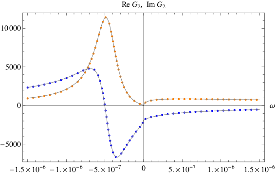
The sharp quasi-particle peaks in the spectral function for spinors were interpreted in [3] as strong indications of underlying Fermi surfaces with Fermi momentum $k_{F}$ . The scaling behavior near a Fermi surface for the parameters range considered there, which all have $\nu_{k_{F}}<{{\frac{1}{2}}}$ , is different from that of the Landau Fermi liquid, suggesting an underlying non-Fermi liquid. Our current discussion allows us to obtain a “landscape” of non-Fermi liquids by scanning all possible values of $m$ and $q$ . Before doing that, let us first make some general comments on the scaling behavior (95)–(100) and the possible underlying non-Fermi liquids:

1.

The form of retarded Green function (91) and scaling behavior (95) again have a nice interpretation in terms of the RG picture described earlier; while the location of the Fermi momentum $k_{F}$ is governed by the UV physics (just like in real solids), the scaling exponents (95) near a Fermi surface are controlled by the dimension of the corresponding operators ${{\mathcal{O}}}_{{\vec{k}}}$ (with $|{\vec{k}}|=k_{F}$ ) in the IR CFT. Note that while the specific value of $\nu_{k_{F}}$ depends on $k_{F}$ as an input parameter, its functional dependence on $k_{F}$ is fixed by the IR CFT.
2.

For $\nu_{k_{F}}<{{\frac{1}{2}}}$ , the corresponding operator in the IR CFT is relevant¹⁸¹⁸ 18 Recall that the dimension in the IR CFT is $\delta_{k_{F}}={{\frac{1}{2}}}+\nu_{k_{F}}$ .¹⁹¹⁹ 19 Note added: The correct notion of ‘relevant’ and ‘irrelevant’ here has been explained in [40]. The pertinent issue is the dimension of the product of the operator in the IR CFT and a free fermion representing the boundstate at the Fermi surface. . From (100), the imaginary part of the pole is always comparable to the real part and thus the quasi-particle is never stable. Also note the ratio (100) depends only on the IR data. Another important feature of the pole is that its residue (96) goes to zero as the Fermi surface is approached. In particular, the smaller $\nu_{k_{F}}$ , the faster the residue approaches zero.
3.

When $\nu_{k_{F}}>{{\frac{1}{2}}}$ , the corresponding operator in the IR CFT is irrelevant. The real part of the dispersion relation (95) is now controlled by the analytic UV contribution and becomes linear with a “Fermi velocity” given by $v_{F}$ . $v_{F}$ is controlled by UV physics and will have to be found numerically by solving the outer region equations (see fig. 7 and discussion of the next subsection). The imaginary part of the pole is still controlled by the dimension of the operator in the IR CFT. In this case the width becomes negligible compared with the real part as the Fermi surface is approached $k_{\perp}\to 0$ , so the corresponding quasi-particle becomes stable. Furthermore the quasiparticle residue is now non-vanishing (96). Note the scaling exponent of the width ${{\Gamma}}$ is generically different from the $\omega^{2}$ -dependence of the Landau Fermi liquid.
4.

When $\nu_{k}={{\frac{1}{2}}}$ , the corresponding operator in the IR CFT is marginal. Now the retarded function is given by (101), in which case the imaginary part of the pole is still suppressed compared to the real part as the Fermi surface is approached, but the suppression is only logarithmic. The quasi-particle residue now vanishes logarithmically as the Fermi surface is approached. Remarkably (101) is precisely of the form postulated in [8] for the “Marginal Fermi Liquid” to describe the optimally doped cuprates. In [8] the term “marginal” referred to the logarithmic vanishing of the quasi-particle weight (residue) approaching the Fermi momentum. Here we see that this term “marginal” is indeed perfectly appropriate.
5.

At $\nu_{k_{F}}=1$ , from (102) the retarded Green function resembles that of a Landau Fermi liquid with the real part of the quasi-particle pole linear in $k_{\perp}$ and the imaginary part quadratic in $k_{\perp}$ . Equation (102), however, has a logarithmic term $\omega^{2}\log\omega$ with a real coefficient which is not present for a Landau Fermi liquid²⁰²⁰ 20 It is amusing to note that a Landau Fermi liquid in $(2+1)$ -d has a logarithmic correction of the form $\omega^{2}\log\omega$ , but with a pure imaginary coefficient (see e.g. [20]).. In particular, this leads to a curious particle-hole asymmetry with a difference in width for a hole and a particle given by²¹²¹ 21 The above asymmetry can also be expressed as ${{{\Gamma}}(\omega_{*}<0)\over{{\Gamma}}(\omega_{*}>0)}=e^{-2\pi qe_{d}}$ .

${{\Gamma}}(\omega_{*}<0)-{{\Gamma}}(\omega_{*}>0)=\pi\tilde{c}_{2}\omega_{*}^{2}\ .$ (107)
6.

Notice from (97) that for all values of $\nu_{k_{F}}$ , $z\geq 1$ . This is consistent with an inequality proposed by Senthil in [7] for a critical Fermi surface.²²²² 22 Senthil derived the inequality $z\geq 1$ by approaching a non-Fermi liquid at the critical point of a continuous metal-insulator transition from the Landau Fermi liquid side and requiring the effective mass should not go to zero as the critical point is approached. In the notation of [7] our Green function (91) also has scaling exponent ${\alpha}=1$ , with $\alpha$ defined as $G_{R}(\lambda^{z}\omega,\lambda k_{\perp})=\lambda^{-\alpha}G_{R}(\omega,k_{\perp})$ . Thus we also have $z\geq{\alpha}$ for all cases, consistent with the other inequality proposed in [7].

For $\nu_{k_{F}}<{{\frac{1}{2}}}$ , equation (91) (with the linear term in $\omega$ omitted) exhibits a particle-hole asymmetry. To characterize this it is convenient to define

\begin{split}{\alpha}_{+}&\equiv-{\theta}_{c}(k_{\perp}>0)={{{\gamma}}_{k_{F}}\over 2\nu_{k_{F}}},\\ {\alpha}_{-}&\equiv{\theta}_{c}(k_{\perp}<0)-\pi={\pi-{{\gamma}}_{k_{F}}\over 2\nu_{k_{F}}}-\pi\end{split}

(108)

with ${\theta}_{c}$ introduced in (99). ${\alpha}_{+}$ gives the angular distance away from the positive real $\omega$ -axis for the pole (i.e. particle-type excitations) at $k_{\perp}>0$ , while ${\alpha}_{-}$ gives the angular distance away from the negative real $\omega$ -axis for the pole (i.e. hole-type excitations) at $k_{\perp}<0$ . From fig. 2 and its caption, ${\alpha}_{\pm}$ are always positive. Their values determine how close the corresponding pole stays to the real axis and hence indicate the sharpness of the resulting peak in the spectral function (i.e. imaginary part of $G_{R}$ ). In particular, when ${\alpha}_{\pm}$ exceeds ${\pi\over 2}$ the corresponding pole moves to the other Riemann sheet²³²³ 23 An example is given in the left plot of fig. 3.. The particle-hole asymmetry is then reflected in the relative magnitudes of ${\alpha}_{\pm}$ . From equation (62) one finds that $2\nu_{k_{F}}{\alpha}_{-}={\rm arg}(1-e^{-2\pi qe_{d}-2\pi i\nu_{k_{F}}})$ which implies ${\alpha}_{-}$ quickly becomes small when $q$ increases as can also be visualized from fig. 2 since the horizontal line of the upper triangle becomes short. In contrast, with some thought one can conclude from fig. 2 that ${\alpha}_{+}$ can only be small when $\nu_{k_{F}}$ is close to ${{\frac{1}{2}}}$ , where ${\alpha}_{-}$ is also small. Away from $\nu_{k_{F}}={{\frac{1}{2}}}$ , one will generically (except for small $q$ ) have a particle-hole symmetry with a sharp peak on the hole side (i.e. small ${\alpha}_{-}$ ), but a broad bump on the particle side (not so small ${\alpha}_{+}$ ). This was indeed what was observed in [3] numerically. The above qualitative features will be confirmed by explicit numerical calculations represented in fig. 6.

8.

Non-Fermi liquids have been described previously by coupling a Fermi surface to a propagating bosonic mode, such as a transverse magnetic excitation of a gauge field, e.g. [22, 23, 24, 25, 26, 27, 28, 29]. The forms of the fermion Green’s functions thus obtained all fit into the set of functions we have found in (91). An important difference, however, is that each of these analyses required a small parameter²⁴²⁴ 24 e.g. $\alpha\sim{1\over 137}$ in [22], $1/N$ in [23], the parameter $x$ in the gauge boson dispersion in [24]… to control the perturbation theory, and the range of frequencies (or temperatures) over which the non-Fermi liquid behavior is relevant is parametrically small in the control parameter. As a result the non-Fermi liquid behavior will only be visible at extremely low temperatures. In our non-perturbative calculation, this range is order unity, and so our non-Fermi liquids may be considered robust versions of these previously-identified phases.

The expression (91) for retarded function near a Fermi surface and the matching procedure from which (91) was derived suggest the following effective action of the UV ${{\mathcal{O}}}_{U}$ and IR ${{\mathcal{O}}}_{I}$ part of an operator ${{\mathcal{O}}}$ (below $|{\vec{k}}_{F}|=k_{F}$ )

	$\displaystyle S=\int d\omega d{\vec{k}}\,\bar{{\mathcal{O}}}_{U}\,\Sigma(\omega,{\vec{k}}_{\perp})\,{{\mathcal{O}}}_{U}\qquad\qquad$
	$\displaystyle+\int d\omega d{\vec{k}}_{F}\,D(\omega,{\vec{k}}_{F})\bar{{\mathcal{O}}}_{U}(\omega,{\vec{k}}_{F})^{\dagger}{{\mathcal{O}}}_{I}(\omega,{\vec{k}}_{F})+h.c.\$		(109)

where $\Sigma(\omega,{\vec{k}}_{\perp})$ represents the kinetic term for ${{\mathcal{O}}}_{U}$ and $D(\omega,{\vec{k}}_{F})$ denotes coupling between ${{\mathcal{O}}}_{I}$ and ${{\mathcal{O}}}_{U}$ . Both $\Sigma$ and $D$ are controlled by UV physics. They are assumed to be real and depend analytically on $\omega$ . We assume that the dynamics of the IR operator ${{\mathcal{O}}}_{I}(\omega,{\vec{k}}_{F})$ is controlled by the IR CFT with two point function given by

{\left\langle{{{\mathcal{O}}}_{I}(\omega,{\vec{k}}_{F})^{\dagger}{{\mathcal{O}}}_{I}(\omega^{\prime},{\vec{k}}_{F}^{\prime})}\right\rangle}_{IR}={{\mathcal{G}}}_{k_{F}}(\omega)\delta_{{\vec{k}}_{F},{\vec{k}}_{F}^{\prime}}\delta(\omega-\omega^{\prime}).

(110)

The action then implies that after summing a geometric series, the full correlation function of ${{\mathcal{O}}}_{U}$ is then given by

G_{R}(\omega,{\vec{k}}_{\perp})={1\over\Sigma(\omega,{\vec{k}}_{\perp})+D^{2}(\omega,{\vec{k}}_{F}){{\mathcal{G}}}_{k_{F}}(\omega)}\

(111)

which has the form of (91). Thus, action (109) gives a phenomenological model of the small-frequency matching procedure described in this paper as a coupling between UV and IR degrees of freedom. This argument is not dissimilar to that taken in [8] to obtain the “marginal Fermi liquid”. It might also be possible to reinterpret the discussion of [22, 23, 24, 25, 26, 27, 28, 29] in this language.

VI.4 The zoo of non-Fermi liquids from gravity

The discussion of previous subsection was based on qualitative features of (91) which are controlled by the IR CFT. To obtain further information regarding properties of the Fermi surface and its low energy excitations we need to work out (numerically) the data which are controlled by UV physics. These include: $k_{F}$ (which then determines $\nu_{k_{F}}$ and ${{\gamma}}_{k_{F}}$ ), $v_{F}$ , $h_{1}$ and $h_{2}$ . We will map out how they depend on the charge $q$ and dimension ${{\Delta}}$ (or equivalently mass $m$ ) of an operator, i.e. the ‘‘phase diagram’’²⁵²⁵ 25 This is an abuse of language because the parameters we are varying are couplings in the bulk action, and hence change the boundary system, not its couplings. of holographic non-Fermi liquids.

In this section we will often use the notations and equations developed in Appendix A. Readers are strongly encouraged to read that part first.

We first solve the Dirac equation (141) numerically with $\omega=0$ to find $k_{F}$ , for which $a_{+}^{(0)}$ defined in equation is (166) is zero. This is equivalent to finding the bound states of the Dirac equation. See Appendix B for more details. For $m\in[0,{{\frac{1}{2}}})$ we consider at the same time the alternative quantization of the bulk spinor field, whose boundary Green function $\tilde{G}_{1,2}(m,k)$ are given by $G_{1,2}(-m,-k)$ (from (153)). We will thus use negative mass to refer to the alternative quantization. The results are presented in fig. 5, where we plotted $k_{F}$ dependence on charge $q$ for three different masses $m=-0.4,\,0,\,0.4$ . Note in this and all subsequent plots if not stated explicitly, we use without loss of generality $R=1$ , $r_{*}=1$ , $g_{F}=1$ and $d=3$ , for which the chemical potential is $\mu=\sqrt{3}$ .

We see in fig. 5 that for a given mass when increasing $q$ new branches of Fermi surfaces appear as was observed before in [3]. This can be understood from the point of view of the Dirac equation as that increasing $q$ allows more bound states. The lowest bound state has the largest $k_{F}$ ,²⁶²⁶ 26 As discussed in Appendix B, the bound state problem for the Dirac equation can be approximately thought of as a Schrodinger problem with eigenvalue $-k^{2}$ . which corresponds to the lowest curves in fig. 5. We will refer it as the ‘primary Fermi surface’. For $q,m$ and $k$ large we can also use the WKB approximation to solve the Dirac equation to find the bound states, which is discussed in detail in Appendix B. In particular, fig. 12 gives the parameter region where there exist Fermi surfaces for large $k_{F},m,q$ for various boundary theory space-time dimensions.

In fig. 6 we map the values of $\nu_{k_{F}}$ , which can be computed from (58), for the primary Fermi surface in the $q$ - $m$ plane. As discussed further in Appendix C, using the wave function for the bound state at $k_{F}$ we can evaluate $v_{F}$ and $h_{1},h_{2}$ . Their values for various masses as a function of $\nu_{k_{F}}$ are presented in fig. 7–fig. 8.

We now summarize some important properties which can be read from these plots and the WKB analysis in Appendix B:

1.

For any $m\geq 0$ and $q$ , in the standard quantization, the existence of Fermi surfaces is always correlated with the existence of the oscillatory region which requires that for any dimension $d$ (c.f. (69))

${{\Delta}}<{|q|g_{F}\over\sqrt{2}}+{d\over 2}\ .$ (112)

This is clear from both fig. 5 and fig. 6 for the masses plotted there. In fact, the allowed region for Fermi surfaces is more stringent than (112). This can be seen from fig. 12 (which follows from the WKB analysis in Appendix B), which indicates that Fermi surfaces only exist for (for any $d$ )

$m^{2}R^{2}<{q^{2}g_{F}^{2}\over 3},\quad{\rm{\it i.e.}\ }\quad{{\Delta}}<{|q|g_{F}\over\sqrt{3}}+{d\over 2}\ .$ (113)

At $m=0$ , in units of the effective chemical potential $\mu_{q}$ , the range for allowed $k_{F}$ is

${d-2\over\sqrt{d(d-1)}}\leq{k_{F}\over\mu_{q}}\leq 1$ (114)

where the lower limit is the boundary of the oscillatory region. The upper limit in (114) also applies to other masses, achieved in the limit $m$ finite, $q\to\infty$ . The lower limits for other masses are smaller than that in (114) as can be seen from fig. 13 (but an analytic expression is not known). Note that for $m$ approaching the allowed limit (113), $k_{F}/\mu_{q}$ lies in a small region around

${k_{F}\over\mu_{q}}={d-2\over\sqrt{3d(d-1)}}\ .$ (115)
2.

For $mR\in(-{{\frac{1}{2}}},0)$ , i.e. for alternative quantization, there exists a single Fermi surface which does not enter the oscillatory region. This is the primary Fermi surface with the largest $k_{F}$ . In fact for the small window

${|q|g_{F}\over\sqrt{2}}<|m|R,$ (116)

i.e. in terms of boundary theory dimension ${{\Delta}}={d\over 2}-|m|R$ ,

${d-1\over 2}<{{\Delta}}<{d\over 2}-{|q|g_{F}\over\sqrt{2}}$ (117)

there exists a Fermi surface without oscillatory region.
3.

For a given $m$ , as one reduces $q$ , $k_{F}$ (and $\nu_{k_{F}}$ ) decreases and eventually loses its Fermi surface identity by entering into the oscillatory region. Similarly, for a given $q$ , as one increases $m$ , $k_{F}$ (and $\nu_{k_{F}}$ ) decreases and eventually enters the oscillatory region.
4.

For a Fermi surface, one can define a topological number using the Green’s function [21]

$n=\textrm{Tr}\oint_{C}{dl\over 2\pi i}G_{R}(k_{\perp},i\omega)\partial_{l}G^{-1}_{R}(k_{\perp},i\omega)$ (118)

which measures the winding of its phase. Here $G_{R}$ should be considered as a matrix in the spinor space and $C$ is any closed loop in the $(k_{\perp},i\omega)$ space around the origin. In our case, for $m=0$ since $\det G_{R}=1$ (see discussion around (155)), i.e. any pole is always canceled by a zero, any Fermi surface has a zero winding. For generic $m\neq 0$ , then Fermi surfaces here generically have $n=\pm 1$ .
5.

Except for the single primary Fermi surface for the alternative quantization, as indicated in the last plot of fig. 5, the Fermi surfaces for the standard and alternative quantizations are paired with the standard quantization have a larger $k_{F}$ . In the limit $mR\to{{\frac{1}{2}}}$ , the paired surfaces for two quantizations now have the same $k_{F}$ .
6.

From fig. 7, for a given mass and $\nu_{k_{F}}>{{\frac{1}{2}}}$ , $v_{F}$ decreases with $\nu_{k_{F}}$ . In particular as $\nu_{k_{F}}\to{{\frac{1}{2}}}$ , $v_{F}$ approaches zero. From the second line of (96) the residue also vanishes in this limit given that $h_{1}$ is regular there (see fig. 8). Also note that as $\nu_{k_{F}}\to\infty$ , $v_{F}\to 1$ .

VI.5 $mR\to-{{\frac{1}{2}}}$ limit and free fermions

We will now consider the $mR\to-{{\frac{1}{2}}}$ limit in some detail (this corresponds to the alternative quantization of $mR={{\frac{1}{2}}}$ ), as in this limit the dimension of the operator approaches that of a free fermion, i.e. in $d$ -dimension, ${{\Delta}}\to{d-1\over 2}$ . Note at exactly $mR=-{{\frac{1}{2}}}$ , the bulk wave function becomes non-normalizable and there does not exist a boundary operator corresponding to it.²⁷²⁷ 27 In other words at $mR={{\frac{1}{2}}}$ there is only one quantization giving rise to a boundary operator of dimension ${{\Delta}}={d+1\over 2}$ . It is natural to ask whether in the limit $mR\to-{{\frac{1}{2}}}$ , the behavior near the Fermi surface approaches that of a Landau Fermi liquid, as recently argued in [4].

We first note the following features as $mR\to-{{\frac{1}{2}}}$ :

1.

In this limit one finds numerically that for the primary Fermi surface, the Fermi momentum approaches the upper limit of (114), i.e.

$k_{F}=\mu_{q}\ .$ (119)
2.

With $k_{F}$ constrained as in (119), by varying $q$ , $\nu_{k_{F}}$ can take any values greater than ${{\frac{1}{2}}}{1\over\sqrt{d(d-1)}}$ .
3.

From (202), one finds that various coefficients in (91) behave as

$h_{1},h_{2}\propto\left(mR+{{\frac{1}{2}}}\right)\to 0,\quad v_{F}\to 1$ (120)

This is due to the fact that at $mR=-{{\frac{1}{2}}}$ , the bound state wave function becomes non-normalizable with a logarithmic divergence. In the limit $mR\to-{{\frac{1}{2}}}$ both $J^{1}$ and $J^{t}$ defined in (198) and (193) are proportional to ${1\over mR+{{\frac{1}{2}}}}$ .

With $h_{2}\to 0$ and $v_{F}\to 1$ , the Green function (91) approaches that of a free relativistic fermion, despite the fact that the non-analytic part can still have a nontrivial exponent $\nu_{k_{F}}$ . Note that equation (119) has a simple interpretation: it is simply the Fermi momentum for a free relativistic fermion with Fermi energy $\mu_{q}$ !

With $h_{1}\to 0$ , the whole Green function vanishes, suggesting that at the same time the fermion disappears in the limit. Note that nowhere along the limit does a Landau Fermi liquid emerge. This picture is consistent with general expectations: in the $mR\to-{{\frac{1}{2}}}$ limit the mode becomes a singleton mode (free fermion) living at the boundary and decoupling from everything else. There are no bulk degrees of freedom associated with it anymore. The fact that we do not see a Landau Fermi liquid emerging in the limit is also consistent with our current understanding of holography; we do not expect a weakly interacting boundary theory to have a bulk description in terms of low energy gravity.

Let us also mention that, at any given mass $mR$ close to $-{{\frac{1}{2}}}$ , $h_{1}$ and $h_{2}$ are small but nonzero. Thus except at parametrically small frequencies (i.e. very close to the Fermi surface), the linear analytic term in (91) will dominate over the non-analytic term. As a result the nontrivial exponent and the fact that the quasi-particle has a finite width will not be easily visible. Turning on a temperature will generate a new width for the quasi-particle and could dominate over the zero-temperature width except at very low temperatures.

In [4] indications were found that there exists a Fermi surface which behaves like a Landau Fermi liquid for $mR$ close to $-{{\frac{1}{2}}}$ at a Fermi energy smaller than $\omega=0$ . This result is surprising, from the following points of view: (i) the Fermi energy is different from (in fact smaller than) the value of the effective chemical potential; (ii) it implies the existence of some kind of fermionic hair outside the black hole at $\omega\neq 0$ ; (iii) from the general philosophy of holography mentioned earlier it is surprising to see a gravity description of a weakly coupled theory. It would be nice to have a better understanding of it. (Note that the small $\omega$ -analysis performed in this paper does not apply to any possible Fermi surfaces at a Fermi energy different from $\omega=0$ .)

Finally, we mention in passing that there is another limit in which free fermions emerge from the WKB analysis. In the limit $q\to\infty$ , with $mR/q$ fixed, again one finds that $h_{2}\to 0$ . In this case, depending on the value $mR/q$ , $v_{F}$ can take a range of values, see fig. 14.

VI.6 Double trace deformation and its effect on Fermi surfaces

As discussed in Appendix A.1, for $mR\in[0,{{\frac{1}{2}}})$ we can turn on a double trace deformation ${{\mathcal{O}}}^{\dagger}{{\mathcal{O}}}$ in the unstable CFT (from the alternative quantization) to flow to the stable CFT. We note that the IR CFT of both CFTs appear to be the same. It is interesting to examine what happens to Fermi surfaces of ${{\mathcal{O}}}$ under this flow. As an example, let us consider $m=0.4$ . By examining the third plot of fig. 5 we observe that in flowing to the stable CFT, the primary Fermi surface (which has the biggest radius) of the unstable one disappears. As a result, for generic $q$ , the number of Fermi surfaces in the stable CFT is one smaller than that in the unstable one. For example, at $q=2$ , one starts in the unstable theory with two Fermi surfaces with radii given by $k_{1}\gg k_{2}$ . In the stable CFT one finds a single Fermi surface at a radius $k_{3}$ which is greater than but comparable to $k_{2}$ , and much smaller than $k_{1}$ . It would be desirable to do a systematic study of more examples.

VII Discussion

In this paper we studied the low frequency expansion of retarded two-point functions of generic charged scalar and spinor operators in a CFT_d at finite charge density using its gravity dual, following the earlier numerical study of [3]. We showed that the spectral functions exhibit various emergent critical behavior controlled by an infrared CFT described by the AdS₂ region of the black hole geometry.

Despite its classical nature, the bulk calculation we performed turned out to have an intimate knowledge of the quantum statistics of the excitations in the boundary theory. In particular, the consistency with the boundary theory statistics dictates that a charged scalar field in the bulk could have various instabilities including superradiance, which are absent for a spinor field. We regard this as a nice indication of the robustness of the AdS/CFT correspondence. We also found a potentially new type of scalar instability which appears to be distinct from the standard tachyon instabilities (including those induced by an electric field).

Our results suggest a nice description for the low energy effective theory near a Fermi surface of a non-Fermi liquid. We find at each point on the Fermi surface, there lives a CFT ²⁸²⁸ 28 As mentioned earlier, the precise nature of the IR CFT is not yet understood. It might be a conformal quantum mechanics or a chiral sector of a $(1+1)$ -dimensional CFT.²⁹²⁹ 29 In fact, the geometry we are studying displays such a CFT even for values of $k$ away from the Fermi surface., parameterized by the angle on the Fermi surface. This is reminiscent of the Fermi liquid picture, except that one replaces the free fermion CFT by a nontrivial one. We found a direct relation between the dimension of an operator in the IR CFT and the scaling exponent of its spectral function; a relevant operator gives rise to unstable quasi-particle excitations at the Fermi surface with a zero quasi-particle weight, while an irrelevant operator gives rise to stable quasi-particles at the Fermi surface with a nonzero quasi-particle weight. We expect this description to be rather general, not restricted to theories with a gravity dual, since it involves nothing more than general concepts of a fixed point. For example, the fact that for marginal operator our expression (101) coincides with that of the “marginal Fermi liquid” description [8] of the optimally doped cuprates may not be an accident and may suggest that the “electron” operator is marginal at the possible quantum critical point describing a optimally doped cuprates.

Note that while in this paper we restricted to a charged black hole in AdS (which corresponds to CFT at a finite charged density), our results should apply to any extremal solution with an AdS₂ region, e.g. that dual to a non-conformal theory at a finite density. One can also put the boundary theory at a finite chemical potential for some components of angular momenta, whose gravity dual is then given by an extremal Kerr-AdS black hole, which has an AdS₂ region.

It is worth comparing the form of our Green’s functions with the well-understood example of a non-Fermi liquid, namely Luttinger liquids in $1+1$ dimensions, This is in some sense a realization of the picture described above, in that to construct a Luttinger liquid one replaces the free fermion CFT of each Fermi point with a free boson of some radius other than the free-fermion radius. It differs from our case in two important ways: First, we don’t know how to obtain the behavior found here as a deformation of the Landau theory. Second, the Green function we find has a non-analyticity at $\omega=0$ for arbitrary $k$ (unlike $G_{{\rm luttinger}}\sim{1\over(k_{\perp}-\omega)^{\nu}}$ ); however, only at $k=k_{F}$ does this non-analyticity represent a peak in the spectral density.

We now discuss two caveats of our study. The first regards the stability of this extremal black hole geometry. While the black hole is by itself thermodynamically and perturbatively stable, as discussed earlier holographic superconductor instabilities³⁰³⁰ 30 As mentioned in footnote 15, a neutral scalar with a sufficient negative mass square can also condense, whose boundary theory interpretation is not yet known. can occur if the gravity theory in which it is embedded contains charged scalars of sufficiently large charge or sufficiently small mass [15, 16, 17, 18]. This might not be of a concern since various physical systems to which we might try to apply the mechanism described here including the normal state of high $T_{C}$ cuprates also exhibit a superconducting instability. Nevertheless, the criteria for a string vacuum which exhibits the fermi surfaces described here but not the superconducting instability are reminiscent of those required of a string vacuum which describes our universe: one doesn’t want light scalar fields³¹³¹ 31 We thank Eva Silverstein for this analogy.. In the latter context, a large machinery [35] has been developed to meet the stated goal, and one can imagine that similar techniques would be useful here. It would also be very interesting to understand how the condensate affects the Fermi surfaces studied here.

As discussed around equation (17), the black hole solution has a finite entropy at zero temperature. Since the semiclassical gravity expression for the entropy is valid in the large $N$ limit, this “ground state degeneracy” may be a consequence of the $N\to\infty$ limit. Given that the solution is not supersymmetric, away from $N=\infty$ (i.e. beyond the gravity approximation) likely these states are energetically closely-spaced, rather than exactly degenerate. It may be useful to compare this situation to that of systems with frustration. While in our geometry this non-vanishing ground-state entropy comes together with the existence of the AdS₂ region which gives rise to the IR CFT description, they in principle reflect different aspects of a system and may not correlate with each other. For example, suppose the CFT₁ dual to AdS₂ can be considered as the right moving sector (with $T_{R}=0$ ) of a $1+1$ -dimensional CFT. Then the nonzero ground state entropy should come from the left-moving sector of this $1+1$ -dimensional CFT with a nonzero left temperature. One can certainly imagine a situation where the left-moving sector is absent, for which case one will then have an IR CFT without a zero-temperature entropy. We should caution that it might be hard for such a situation to arise as the near horizon limit of a classical gravity solution.

Our results can be generalized in a variety of ways. The most immediate is finite temperature, which should shed further light on the structure of CFT₁. It will be interesting to follow the instability for scalars to the critical temperature [18]. It is also instructive to examine the two-point functions of charge current and density fluctuations. They correspond to fluctuations of the bulk gauge field $A_{M}$ in the transverse and longitudinal channel respectively. Here we expect even at zero temperature there exist hydrodynamic modes like diffusion and sound modes as this is a non-neutral plasma and dissipates even at zero temperature (e.g. it has a finite entropy). We expect our master formula (55) still applies after having diagonalized the perturbations. In particular the diffusion and sound modes will depend on the small $k$ expansion of $a_{+}^{(0)}$ , i.e. it should have a zero at $k=0$ .

The matching behavior between the inner region and outer region is very reminiscent of that for the D3-D7 system at small densities in [37]. There the geometry is more complicated and does not directly give a hint what would be the IR theory. Nevertheless it appears likely the IR theory there is a non-relativistic CFT at finite density.

Acknowledgements

We thank A. Adams, S. Hartnoll, M. Hermele, G. Horowitz, N. Iqbal, S. Kachru, A. Karch, Z. Komargodski, M. Lawler, P. Lee, S-S. Lee, J. Maldacena, J. Polchinski, K. Rajagopal, S. Sachdev, N. Seiberg, E. Silverstein, G. Shiu, S. Sondhi, S. Trivedi and in particular T. Senthil for valuable discussions and encouragement. HL would also like to thank the physics department at UCSB for hospitality during the last stage of this work. Work supported in part by funds provided by the U.S. Department of Energy (D.O.E.) under cooperative research agreement DE-FG0205ER41360 and the OJI program. The research was supported in part by the National Science Foundation under Grant No. NSF PHY05-51164.

Appendix A Spinor calculation

A.1 Remarks on dictionary

A bulk Dirac spinor field $\psi$ with charge $q$ is mapped to a fermionic operator ${{\mathcal{O}}}$ in CFT of the same charge. ${{\mathcal{O}}}$ is a Dirac spinor for $d$ odd, and a chiral spinor for $d$ even [33]. In both cases the dimension of the boundary spinor ${{\mathcal{O}}}$ is half of that of $\psi$ . Since $\psi$ has $2^{[{d+1\over 2}]}$ complex components, where $[x]$ denotes the integer part of $x$ , the boundary retarded Green function $G_{R}$ for ${{\mathcal{O}}}$ is a $2^{[{d-1\over 2}]}\times 2^{[{d-1\over 2}]}$ matrix. The conformal dimension ${{\Delta}}$ of ${{\mathcal{O}}}$ is given in terms of the mass $m$ of $\psi$ by³²³² 32 Without loss of generality in this paper we will take $m\geq 0$ . For negative $m$ the discussion is exactly parallel, with $m$ replaced by $|m|$ . For odd $d$ the Dirac equation for $-m$ is completely equivalent to $m$ as one can change the sign of mass by taking $\psi\to{{\Gamma}}\psi$ where ${{\Gamma}}$ is the $d+1$ -dimensional chirality matrix. For $d$ even, different signs of $m$ corresponds to different chirality of ${{\mathcal{O}}}$ .

{{\Delta}}={d\over 2}\pm mR\

(121)

where $R$ is the AdS curvature radius. In (121), one should use the $+$ sign for $mR\geq{{\frac{1}{2}}}$ . For $mR\in[0,{{\frac{1}{2}}})$ , there are two ways to quantize $\psi$ by imposing different boundary conditions at the boundary, which corresponds to two different CFTs. We will call the CFT in which ${{\mathcal{O}}}$ has dimension ${{\Delta}}={d\over 2}+mR$ the “stable” CFT and the one with dimension $\tilde{{\Delta}}={d\over 2}-mR\in({d-1\over 2},{d\over 2}]$ the “unstable” CFT. In the “unstable” CFT, the double trace operator ${{\mathcal{O}}}^{\dagger}{{\mathcal{O}}}$ produces a relevant deformation under which the theory flows to the “stable” CFT [30].

The retarded Green function of ${{\mathcal{O}}}$ at finite charge density can be extracted by solving the Dirac equation for $\psi$ in the charged AdS black hole geometry.

A.2 Dirac equation

We consider a spinor field in the black hole geometry (2) with a quadratic action

S=\int d^{d+1}x\sqrt{-g}\,i(\bar{\psi}{{\Gamma}}^{M}{{\mathcal{D}}}_{M}\psi-m{\bar{\psi}}\psi)

(122)

where ${\bar{\psi}}=\psi^{\dagger}{{\Gamma}}^{\underline{t}}$ and

{{\mathcal{D}}}_{M}=\partial_{M}+{1\over 4}\omega_{abM}{{\Gamma}}^{ab}-iqA_{M}\

(123)

with $\omega_{abM}$ the spin connection. Our notations are as follows. We will use $M$ and $a,b$ to denote abstract bulk spacetime and tangent space indices respectively, and $\mu,\nu\cdots$ to denote indices along the boundary directions, i.e. $M=(r,\mu)$ . Underlined indices on Gamma matrices always refer to tangent space ones.

Writing

\psi=(-gg^{rr})^{-{1\over 4}}e^{-i\omega t+ik_{i}x^{i}}\Psi

(124)

the corresponding Dirac equation for $\psi$ can be written as

\sqrt{g_{ii}\over g_{rr}}\left({{\Gamma}}^{\underline{r}}\partial_{r}-m\sqrt{g_{rr}}\right)\Psi+iK_{\mu}{{\Gamma}}^{\underline{\mu}}\Psi=0,

(125)

with

K_{\mu}(r)=\left(-u(r),k_{i}\right)

(126)

and $u(r)$ is given by

u=\sqrt{g_{ii}\over-g_{tt}}\left(\omega+\mu_{q}\left(1-{r_{0}^{d-2}\over r^{d-2}}\right)\right)\ .

(127)

As in the case of a charged boson, equation (125) depends on $q$ and $\mu$ only through the combination

\mu_{q}\equiv\mu q

(128)

which is the effective chemical potential for a field of charge $q$ . Similarly, $\omega$ should be identified with frequency measured away from the the effective chemical potential (128). Due to rotational symmetry in the spatial directions, we do not lose generality by setting

k_{1}=k,\qquad k_{i}=0,\quad i\neq 1\ .

(129)

Notice that equation (125) then only depends on three Gamma matrices ${{\Gamma}}^{\underline{r}},{{\Gamma}}^{\underline{t}},{{\Gamma}}^{\underline{1}}$ . As a result³³³³ 33 For general $k_{i}$ the projector can be written as $\Pi^{\hat{k}}_{\pm}\equiv{\frac{1}{2}}\left(1\pm\Gamma^{{\underline{r}}}\Gamma^{{\underline{t}}}\hat{k}_{i}\Gamma^{{\underline{i}}}\right),$ (130) where $\hat{k}_{i}$ is the unit vector $\hat{k}\equiv\vec{k}/|\vec{k}|$ . projectors

\Pi_{\alpha}\equiv{\frac{1}{2}}\left(1-(-1)^{\alpha}\Gamma^{{\underline{r}}}\Gamma^{{\underline{t}}}\Gamma^{\underline{1}}\right),\;{\alpha}=1,2,\quad\Pi_{1}+\Pi_{2}=1

(131)

commute with the Dirac operator of (125) and

\Phi_{\alpha}=\Pi_{\alpha}\Psi,\quad{\alpha}=1,2

(132)

decouple from each other. It is then convenient to write $\Phi=\left(\begin{matrix}\Phi_{1}\cr\Phi_{2}\end{matrix}\right)$ and choose the following basis of Gamma matrices

	$\displaystyle{{\Gamma}}^{\underline{r}}=\left(\begin{array}[]{cc}-\sigma^{3}{\bf 1}&0\\ 0&-\sigma^{3}{\bf 1}\end{array}\right),\;\;{{\Gamma}}^{\underline{t}}=\left(\begin{array}[]{cc}i\sigma^{1}{\bf 1}&0\\ 0&i\sigma^{1}{\bf 1}\end{array}\right),$
	$\displaystyle{{\Gamma}}^{\underline{1}}=\left(\begin{array}[]{cc}-\sigma^{2}{\bf 1}&0\\ 0&\sigma^{2}{\bf 1}\end{array}\right),\qquad\cdots$

under which the Dirac equation (125) becomes

\left(\partial_{r}+m\sqrt{g_{rr}}\sigma^{3}\right)\Phi_{\alpha}=\sqrt{g_{rr}\over g_{ii}}\left(i\sigma^{2}u+(-1)^{\alpha}k\sigma^{1}\right)\Phi_{\alpha}\ .

(141)

In equation (A.2), ${\bf 1}$ is an identity matrix of size $2^{d-3\over 2}$ for $d$ odd (or size $2^{d-4\over 2}$ for $d$ even); since the resulting Green’s functions will also be proportional to such an identity matrix, we will suppress them below. Note that (A.2) is chosen so that equation (141) is real for real $\omega,k$ .

Near the boundary, (141) has two linearly independent solutions given by (with $1/r$ subleading terms for each solution suppressed)

\Phi_{\alpha}\mathrel{\mathop{\kern 0.0pt\approx}\limits^{r\to\infty}}a_{\alpha}r^{mR}\left(\begin{matrix}0\cr 1\end{matrix}\right)+b_{\alpha}r^{-mR}\left(\begin{matrix}1\cr 0\end{matrix}\right)\qquad{\alpha}=1,2\ .

(142)

To compute the retarded functions, one should impose the in-falling boundary condition for $\Phi$ at the horizon. Then the boundary spinor Green functions have two sets of eigenvalues given by³⁴³⁴ 34 That is, when diagonalized, the boundary retarded functions have the form $G_{R}(\omega,k)=\left(\begin{array}[]{cc}G_{1}(\omega,k){\bf 1}&0\\ 0&G_{2}(\omega,k){\bf 1}\end{array}\right)\ .$ (143)

G_{\alpha}(\omega,k)={b_{\alpha}\over a_{\alpha}}\ ,\quad{\alpha}=1,2\ .

(144)

To see (144), consider spinors $\phi_{\pm}={{\frac{1}{2}}}(1\pm{{\Gamma}}^{\underline{r}})\Phi$ with definite eigenvalues of ${{\Gamma}}^{\underline{r}}$ . Then

{\rm with}\quad\Phi_{\alpha}\equiv\left(\begin{matrix}y_{\alpha}\cr z_{\alpha}\end{matrix}\right),\qquad\phi_{+}=\left(\begin{matrix}z_{1}\cr z_{2}\end{matrix}\right),\quad\phi_{-}=\left(\begin{matrix}y_{1}\cr y_{2}\end{matrix}\right)

(145)

where we have suppressed zero entries in $\phi_{\pm}$ . Equation (144) then follows using the prescription of [33] (see e.g. sec. IIIB).³⁵³⁵ 35 A note on notation: compared to the notation of [3], $\Phi_{1}\equiv\left(\begin{matrix}iy_{-}\cr z_{+}\end{matrix}\right),~~\Phi_{2}\equiv\left(\begin{matrix}-iz_{-}\cr y_{+}\end{matrix}\right)~.$

The dictionary (144) is for the conventional quantization which applies to any $m\geq 0$ . For $mR\in[0,{{\frac{1}{2}}})$ , there is also an alternative quantization, as discussed at the beginning of this section. Similar argument then leads to

\tilde{G}_{\alpha}=-{a_{\alpha}\over b_{\alpha}}=-{1\over G_{\alpha}}.

(146)

A.3 Some properties of the spinor correlators

In (141) the equation for $\Phi_{2}$ is related to that of $\Phi_{1}$ by $k\to-k$ , so we immediately conclude that

G_{2}(\omega,k)=G_{1}(\omega,-k)\ .

(147)

As a result the trace and determinant of $G_{R}$ are invariant under $k\to-k$ as should be the case. Given (147), from now on we will focus solely on $G_{1}(\omega,k)$ . For notational simplicity, we will also drop the subscript ${\alpha}=1$ below. Unless written explicitly all relevant quantities should be interpreted as having a subscript ${\alpha}=1$ .

More properties of $G$ can be derived from (141). For this purpose it is convenient to write (144) as³⁶³⁶ 36 In (148) one should extract the finite terms in the limit.

G=\lim_{\epsilon\to 0}\epsilon^{-2mR}\xi|_{r={1\over\epsilon}},\quad{\rm with}\quad\xi\equiv{y\over z}\ .

(148)

From (141), as in [32] one can then derive a flow equation for $\xi$ ,

\sqrt{g_{ii}\over g_{rr}}\partial_{r}\xi=-2m\sqrt{g_{ii}}\xi+(u-k)+(u+k)\xi^{2}

(149)

with in-falling boundary condition at the horizon given by (for $\omega\neq 0$ )

\xi|_{r=r_{0}}=i\ .

(150)

Properties of $G$ can now be read from those of (149). By taking $q\to-q,\omega\to-\omega,k\to-k$ and $\xi\to-\xi$ we find that the equation for $\xi$ goes back to itself, implying

G(\omega,k;q)=-G^{*}(-\omega,-k;-q)\

(151)

where the complex conjugation is due to that with $\omega\to-\omega$ the infalling horizon boundary condition turns into the outgoing one, which can then be changed back by a complex conjugation.

By dividing both sides of equation (149) by $\xi^{2}$ , we obtain an identical equation for $-{1\over\xi}$ if we also take $m\to-m,k\to-k$ . This implies that

G(\omega,k;-m)=-{1\over G(\omega,-k;m)}\ .

(152)

Given equation (146) we conclude that for alternative quantization $\tilde{G}$ can be written as

\tilde{G}(\omega,k;m)=G(\omega,-k;-m)\ .

(153)

That is, alternative quantization can be included by extending the mass range for $G(\omega,k;m)$ from $m\geq 0$ to $mR>-{{\frac{1}{2}}}$ . Below and in the main text when we speak of negative mass it should be understood that it refers to the alternative quantization.

For $m=0$ , from (152) and (147), we find that

G_{2}(\omega,k)=-{1\over G_{1}(\omega,k)},\qquad m=0\

(154)

which implies that

\det G_{R}(\omega,k)=1,\qquad m=0

(155)

Note that since a basis change and a Lorentz rotation do not change the determinant of $G_{R}$ , equation (155) applies to any basis of Gamma matrices and any momentum. Combining (147) and (154) we also conclude that at $k=0$ ,

G_{1}(\omega,k=0)=G_{2}(\omega,k=0)=i,\quad m=0\ .

(156)

Also note that equation (154) implies that for $m=0$ the alternative quantization is equivalent to original one [33].

A.4 Small-frequency expansion

In this subsection, we present the low-frequency expansion analysis of section III adapted to the case of a spinor field. Now the equation is given by (141) with ${\alpha}=1$ which we copy here for convenience

\left(\partial_{r}+m\sqrt{g_{rr}}\sigma^{3}\right)\Phi=\sqrt{g_{rr}\over g_{ii}}\left(i\sigma^{2}u-k\sigma^{1}\right)\Phi\ .

(157)

We will again divide the $r$ -axis into two regions as (37)–(38) and consider the low frequency limit (39). The story is very much parallel, so we will be brief.

In the inner region, to leading order in $\omega$ -expansion equation (157) reduces to equation (235) of a spinor field in AdS₂ with $\tilde{m}=-(-1)^{\alpha}{kR\over r_{*}}$ . All the discussion in sec. D.2 can now be carried over with the replacement $\nu\to\nu_{k}$

\nu_{k}\equiv\sqrt{m_{k}^{2}R_{2}^{2}-e_{d}^{2}q^{2}-i\epsilon},\quad m_{k}^{2}\equiv m^{2}+{k^{2}R^{2}\over r_{*}^{2}}\ .

(158)

For example, near the boundary of the inner region, i.e. ${\omega R_{2}^{2}\over r-r_{*}}\to 0$ , the leading order inner solution can be expanded as

\Phi_{I}^{(0)}(\omega,{\vec{k}};\zeta)=v_{-}\left({R_{2}^{2}\over r-r_{*}}\right)^{-\nu_{k}}\;\;+\;\;{{\mathcal{G}}}_{k}(\omega)v_{+}\left({R_{2}^{2}\over r-r_{*}}\right)^{\nu_{k}}

(159)

where $v_{\pm}$ and ${{\mathcal{G}}}_{k}$ can be obtained respectively from (240) and (242). More explicitly,

v_{\pm}=\left(\begin{matrix}mR_{2}\pm\nu_{k}\cr{kR\over r_{*}}R_{2}+qe_{d}\end{matrix}\right)\ ,

(160)

and

	$\displaystyle{{\mathcal{G}}}_{k}(\omega)$	$\displaystyle=$	$\displaystyle e^{-i\pi\nu_{k}}\frac{\Gamma(-2\nu_{k})\,\Gamma\left(1+\nu_{k}-iqe_{d}\right)}{\Gamma(2\nu_{k})\,\Gamma\left(1-\nu_{k}-iqe_{d}\right)}$		(161)
		$\displaystyle\times$	$\displaystyle\;\frac{\left(m-{ikR\over r_{}}\right)R_{2}-iqe_{d}-\nu_{k}}{\left(m-{ikR\over r_{}}\right)R_{2}-iqe_{d}+\nu_{k}}\;\omega^{2\nu_{k}}\ .$		(162)

As discussed around (240), ${{\mathcal{G}}}_{k}$ depends on the normalizations of $v_{\pm}$ in (160). But it can be checked explicitly that the final correlation function (55) is independent of the normalizations.

In the outer region we can then choose the two linearly independent solutions for the zero-th order equation (i.e. (141) with $\omega=0$ ) by the boundary conditions

\eta_{\pm}^{(0)}=v_{\mp}\left(r-r_{*}\over R_{2}^{2}\right)^{\pm\nu_{k}}+\cdots,\qquad r-r_{*}\to 0\ .

(163)

The matching, the generalization to higher orders in $\omega$ , and the low frequency expansion of $G_{R}$ now work completely in parallel as those for scalar fields. More explicitly, perturbatively in $\omega$ the full outer solution $\Phi_{O}$ can be written as

\Phi_{O}=\eta_{+}+{{\mathcal{G}}}_{k}(\omega)\eta_{-}

(164)

with

\eta_{\pm}=\eta^{(0)}_{\pm}+\omega\eta^{(1)}_{\pm}+\omega^{2}\eta^{(2)}_{\pm}+\cdots\ .

(165)

$\eta^{(n)}_{\pm},n\geq 1$ are obtained from solving (157) perturbatively in the outer region and are uniquely specified by requiring that when expanded near $r=r_{*}$ , they do not contain any terms proportional to the zeroth order solutions (163). Now expanding various $\eta^{(n)}_{\pm},n\geq 0$ near $r\to\infty$ as in (142)

\eta^{(n)}_{\pm}\mathrel{\mathop{\kern 0.0pt\approx}\limits^{r\to\infty}}a_{\pm}^{(n)}r^{mR}\left(\begin{matrix}0\cr 1\end{matrix}\right)+b_{\pm}^{(n)}r^{-mR}\left(\begin{matrix}1\cr 0\end{matrix}\right)

(166)

then the retarded function $G$ is again given by the master formula (55).

Appendix B Bound states at $\omega=0$ and WKB

B.1 Scalar bound states

Setting $\omega=0$ in (33) defines the outer region differential equation for the scalar field. We are then interested in examining normalizable solutions to this equation, since this tells us about the spectrum of excitations of the boundary theory. This is equivalent to studying solutions to this differential equation with boundary conditions (48) for $\eta^{(0)}_{+}$ and $a_{+}^{(0)}=0$ in (54). The alternative quantization window can be achieved by studying $b_{+}^{(0)}=0$ . As we will see, bound states will exist for a discrete set of momenta, so (at least for the fermion problem) these excitations will define a Fermi surface.

We will study the spinor problem in the next subsection. For now the scalar problem will suffice since this problem is probably be more intuitive.

By scaling the wave function and redefining the radial coordinate, $\phi(r)=Z\psi(s)$ , the wave equation (33) can be put in the form,

-\partial_{s}^{2}\psi+V(s)\psi=(-k^{2})\psi

(167)

where the “tortoise” coordinate and the rescaling are,

\frac{ds}{dr}=\sqrt{\frac{g_{rr}}{g_{ii}}}\,,\qquad Z=\left(\frac{g_{rr}g_{ii}}{-g}\right)^{1/4}

(168)

In doing this we have defined a unique Schrödinger potential for this problem:

V=\left(-u^{2}+m^{2}g_{ii}\right)+\left((\partial_{s}\ln Z)^{2}-\partial_{s}^{2}\ln Z\right)

(169)

The problem is to find bound states in this potential with negative “energy” $E=-k^{2}$ . Pictures of this potential are shown in Fig. 11 for fixed $m^{2}$ and various values of $q$ . Examining the $r\rightarrow r_{*}$ limit, which corresponds to $s\rightarrow-\infty$ we find that the potential goes to a constant

V(s)\rightarrow\frac{r_{*}^{2}}{R^{2}R_{2}^{2}}(-(qe_{d})^{2}+m^{2}R_{2}^{2}+1/4)

Hence there exists a continuum near the horizon for momentum satisfying $-k^{2}>\frac{r_{*}^{2}}{R^{2}R_{2}^{2}}(-(qe_{d})^{2}+m^{2}R_{2}^{2}+1/4)$ . This is the criterion for the oscillatory region. That is, we have identified the oscillatory behavior as arising from the existence of a continuum.

Bound states then exist if the potential well in Fig. 11 close to $s=0$ is deep enough. The “sprouting” of bound states out of the oscillatory region in the $q-k$ plot of Fig. 5 has a nice interpretation in terms of developing new bound states as the potential well varies.

B.2 Spinor bound states

The bound state problem is now the first order Dirac equation:

\sqrt{g_{ii}g^{rr}}\partial_{r}\Phi=\begin{pmatrix}-(m/R)r&-k+u\\ -k-u&(m/R)r\end{pmatrix}\Phi

(170)

subject to normalizability conditions for $\eta^{(0)}_{+}$ in (163) and $a_{+}^{(0)}=0$ in (166).

It is harder to have an intuitive grasp over this equation, as in the second order problem. We can of course square this operator to obtain a Schrödinger problem, but there seems to be no way to define a unique potential, such as the one for the scalar. We proceed with an arbitrary choice, in order to give a qualitative understanding of the existence of bound states.

Taking $\Phi=(y,z)^{T}$ we can write (170) as

	$\displaystyle\sqrt{g_{ii}g^{rr}}Q^{-1}\partial_{r}\left(Qy\right)$	$\displaystyle=$	$\displaystyle(u-k)z$		(171)
	$\displaystyle\sqrt{g_{ii}g^{rr}}Q\partial_{r}\left(Q^{-1}z\right)$	$\displaystyle=$	$\displaystyle-(k+u)y$		(172)

where $Q=\exp\left(m\int dr\sqrt{g^{ii}g_{rr}}mr/R\right)$ . Then we can write a second order differential equation for $\psi=z/Q$ . Defining a new tortoise coordinate:

\frac{ds_{F}}{dr}=\sqrt{\frac{g_{rr}}{g_{ii}}}\frac{1+u/k}{Q^{2}}

(173)

we find a zero-energy Schrödinger equation,

-\partial_{s_{F}}^{2}\psi+V_{F}\psi=0,\qquad(V_{F})/k^{2}=\frac{1-u/k}{1+u/k}Q^{4}

(174)

Pictures of this potential are shown in Fig. 11 for 3 different fixed values of $m$ and various values of $\mu_{q}/k$ . Note in Fig. 11 $k$ has been scaled out of the potential, so one should imagine scaling the potential by dialing $k$ to find when a bound states energy eigenvalue crosses zero, this will define the fermi momentum $k_{F}$ . In particular for a given value of $\mu_{q}/k$ there are possibly an infinite set of bound states energies which cross zero as $k$ is increased.

Examining the behavior close to the horizon the tortoise coordinate behaves as $s_{F}\rightarrow-\infty$ for $m\geq 0$ and $s_{F}\rightarrow s_{*}$ for $m<0$ . The potential is of the form $c/s_{F}^{2}$ for $m>0$ and $c/(s_{F}-s_{*})^{2}$ for $m<0$ where

c=\frac{\left(k^{2}R^{2}R_{2}^{2}/r_{*}^{2}-(qe_{d})^{2}\right)}{4m^{2}R_{2}^{2}}

(175)

so that the condition for being in the oscillatory region is the usual condition for a singular $c/s^{2}$ potential in quantum mechanics: $c<-1/4$ .

B.3 WKB analysis

We can analyze both the scalar field and spinor under various limits using WKB analysis. We will focus here on the limit $q,k,m\rightarrow\infty$ with ratios $k/q$ and $k/m$ fixed and consider the scalar and spinor problems in parallel. A useful reference for the application of WKB to the Dirac equation is [36].

As we will see, both problems are governed by the “WKB momentum”

p^{2}=k^{2}+(m^{2}/R^{2})r^{2}-u^{2}

(176)

For the scalar field, this is simply the usual potential-minus-energy term $V-(-k^{2})$ from (169) where terms which depend on $Z$ are small so should be dropped. For the spinor it is the negative of the determinant of the matrix on the rhs of (170). The sign of $p^{2}$ will tell us if we are in the classically allowed ( $p^{2}<0$ ) or disallowed ( $p^{2}>0$ ) region. Note that $p^{2}\sim\mathcal{O}(k^{2})$ is large in the WKB approximation. In the parameter space shown in Fig. 12, there are two turning points $r_{1},r_{2}$ , with a classically allowed region in between the two. The WKB approximation to the wave function in the three regions is:

•

$r<r_{1}$ and $r>r_{2}$ (we use a compact notation to write both these regions together, with $1,2$ correlated with $\pm$ in a self explanatory way)

$\displaystyle\psi(r)$	$\displaystyle=$	$\displaystyle\frac{C^{B}_{1,2}}{\sqrt{p}}\exp\left(\pm\int_{r_{1,2}}^{r}dr^{\prime}\sqrt{g^{ii}g_{rr}}p(r^{\prime})\right)$	(177)
$\displaystyle\Phi(r)$	$\displaystyle=$	$\displaystyle\frac{C^{F}_{1,2}}{\sqrt{p(k+u)}}\begin{pmatrix}mr/R\mp p\\ k+u\end{pmatrix}\times$	(178)
		$\displaystyle\times\exp\left(\pm\int_{r_{1,2}}^{r}dr^{\prime}\left(\sqrt{g^{ii}g_{rr}}p(r^{\prime})+\chi(r^{\prime})\right)\right)$	(178)

where $\chi$ is an $\mathcal{O}(1)$ function given by,

\chi(r^{\prime})=\frac{k+u(r^{\prime})}{2p(r^{\prime})}\partial_{r^{\prime}}\left(\frac{mr^{\prime}/R}{k+u(r^{\prime})}\right)

(179)

•

$r_{1}<r<r_{2}$

	$\displaystyle\hskip-19.91684pt\psi(r)\hskip-2.84544pt$	$\displaystyle=$	$\displaystyle\hskip-2.84544pt\frac{D_{B}}{\sqrt{\rho}}\mathrm{Re}\left\{e^{i\theta_{B}(r_{1},r)+i\xi}\right\}$		(180)
	$\displaystyle\hskip-19.91684pt\Phi(r)\hskip-2.84544pt$	$\displaystyle=$	$\displaystyle\hskip-5.69046pt\frac{D_{F}}{\sqrt{\rho(k+u)}}\mathrm{Re}\left\{\begin{pmatrix}mr/R-i\rho\\ k+u\end{pmatrix}e^{i\theta_{F}(r_{1},r)+i\xi}\right\}$		(181)

where $\rho^{2}=-p^{2}$ and,

$\displaystyle\hskip-25.6073pt\theta_{B}(r_{1},r)$	$\displaystyle=$	$\displaystyle\int_{r_{1}}^{r}dr^{\prime}\sqrt{g^{ii}g_{rr}}\rho(r^{\prime})$	(182)
$\displaystyle\hskip-25.6073pt\theta_{F}(r_{1},r)$	$\displaystyle=$	$\displaystyle\theta_{B}(r_{1},r)$	(183)
		$\displaystyle-\int_{r_{1}}^{r}dr^{\prime}\frac{k+u(r^{\prime})}{2\rho(r^{\prime})}\partial_{r^{\prime}}\left(\frac{mr^{\prime}}{k+u(r^{\prime})}\right)$	(183)

We can formulate a quantization condition by matching the integration constants (in particular $\xi=-\pi/4$ ) across the turning points using Airy functions. The quantization conditions for the scalar and spinor problem turn out to be,

	$\displaystyle\pi(n+1/2)$	$\displaystyle=$	$\displaystyle\theta_{B}(r_{1},r_{2})$		(184)
	$\displaystyle\pi(n+1/2)$	$\displaystyle=$	$\displaystyle\theta_{F}(r_{1},r_{2})$		(185)

respectively. Note that the quantization condition for the spinor only works for $m>0$ , and no information on the alternative quantization region for either spinor or scalar can be found with this analysis.

Using (185) in Fig.. 13 we plot contours of fixed $\nu$ and $q$ in the WKB parameter region for $n=0$ . We note that the validity of the WKB approximation is for $n$ large, however it seems to work remarkably well for $n=0$ the ground state. One might also imagine that it might be exact for $n=0$ when the quantization condition forces us into the limit $k_{F},q,m\rightarrow\infty$ . Such a situation does occur at to the upper boundary of Fig. 13 when $r_{1}\rightarrow r_{2}$ . Actually more care is required in this limit: for the scalar field we can formulate a scaling limit in which the potential becomes that of a simple harmonic oscillator (SHO) located at the radius where $r_{1}\rightarrow r_{2}$ . In this case, the WKB quantization condition should be exact since it is exact for the SHO. Unfortunately it seems hard to find the equivalent scaling limit for the spinor, see Sec.C.3 for more discussion of this.

Appendix C Formulas for $v_{F},h_{1},h_{2}$

C.1 Spinors

In this section we will derive general formulas for various coefficients appearing in equation (91). These coefficients are of great importance in characterizing physical properties of the Fermi surface as they determine the Fermi velocity, the locations of quasi-particle poles, and the residues at the poles. The following discussion will be very similar to the derivation of the Feynman-Hellmann theorem, which (not coincidentally) is commonly used to determine dispersion relations in e.g. photonic crystals [38]. We will focus on the spinor case, and comment on the corresponding result for the charged scalar at the end.

Consider the Dirac equation from (122)

({{\Gamma}}^{M}{{\mathcal{D}}}_{M}-m)\psi=0

(186)

in Fourier space where the Dirac operator ${{\mathcal{D}}}$ depends on $\omega$ and $k$ , which we will collectively denote as $\lambda$ . Now suppose that (186) has a solution $\psi_{0}$ for $\lambda=\lambda_{0}$ , i.e.

({{\Gamma}}^{M}{{\mathcal{D}}}_{M}|_{\lambda_{0}}-m)\psi_{0}=0\ .

(187)

Consider varying $\lambda_{0}\to\lambda_{0}+\delta\lambda$ with the corresponding solution to (186) given by $\psi_{0}+\delta\lambda\psi_{1}$ . $\psi_{1}$ then satisfies

({{\Gamma}}^{M}{{\mathcal{D}}}_{M}|_{\lambda_{0}}-m)\psi_{1}+\left.{{\Gamma}}^{M}{\partial{{\mathcal{D}}}_{M}\over\partial\lambda}\right|_{\lambda_{0}}\psi_{0}=0\ .

(188)

Multiplying (188) on the left by $\int_{r_{*}}^{\infty}dr\,\sqrt{-g}\bar{\psi}_{0}$ , integrating by parts, and using (187), we find that

W(\infty)-W(r_{*})+\int_{r_{*}}^{\infty}dr\,\sqrt{-g}\,\bar{\psi}_{0}{{\Gamma}}^{M}{\partial{{\mathcal{D}}}_{M}\over\partial\lambda}\psi_{0}=0

(189)

where

W=\sqrt{-g}\bar{\psi}_{0}{{\Gamma}}^{r}\psi_{1}\ .

(190)

We will now be more specific, taking $\lambda=\lambda_{0}$ corresponding to $\omega=0,k=k_{F}$ and $\psi_{0}$ to be that corresponding to $\eta_{+}^{(0)}$ defined in (163), i.e. from (124) $\psi_{0}=(-gg^{rr})^{-{1\over 4}}\eta_{+}^{(0)}$ . Recall that at $k=k_{F}$ , $\eta_{+}^{(0)}$ is normalizable with $a_{+}^{(0)}=0$ . We will now consider small $\omega$ and $k$ variations separately:

Take $\lambda=\omega$ in (189). Then we have $\psi_{1}=(-gg^{rr})^{-{1\over 4}}\eta_{+}^{(1)}$ , where $\eta_{+}^{(1)}$ was introduced in (165), and $W=\bar{\eta}_{+}^{(0)}{{\Gamma}}^{{\underline{r}}}\eta_{+}^{(1)}$ . Equation (189) then becomes

ib_{+}^{(0)}a_{+}^{(1)}-\left(\bar{\eta}_{+}^{(0)}{{\Gamma}}^{{\underline{r}}}\eta_{+}^{(1)}\right)\bigr|_{r_{*}}-iJ^{t}|_{\psi_{0}}=0

(191)

with

	$\displaystyle J^{t}\|_{\psi_{0}}$	$\displaystyle=$	$\displaystyle\int_{r_{*}}^{\infty}dr\,\sqrt{-g}\,\bar{\psi}_{0}{{\Gamma}}^{t}\psi_{0}$		(192)
		$\displaystyle=$	$\displaystyle-\int_{r_{*}}^{\infty}dr\,(-g_{rr}g^{tt})^{{\frac{1}{2}}}\,(\eta_{+}^{(0)})^{\dagger}\eta_{+}^{(0)}\ .$		(193)

where in obtaining (191) we have used (166) and (A.2). Note that near $r\to r_{*}$ , $\eta_{+}^{(0)}\sim(r-r_{*})^{\nu_{k}}$ , thus

J^{t}\propto{1\over 2\nu_{k}-1},\quad\nu_{k}\to{{\frac{1}{2}}}

(194)

and becomes divergent from integration near $r_{*}$ when $\nu_{k}\leq{{\frac{1}{2}}}$ . Since the first term in (191) is a finite constant, the divergence has to be canceled by the second term in (191). As can be checked explicitly the second term in (191) is indeed divergent³⁷³⁷ 37 Near $r\to r_{*}$ , $\eta^{(1)}_{+}\sim(r-r_{*})^{\nu_{k}-1}$ . for $\nu_{k}\geq{{\frac{1}{2}}}$ and precisely cancels that of $J^{t}$ . For $\nu_{k}<{{\frac{1}{2}}}$ the boundary contribution from the horizon vanishes. Thus we find that

a_{+}^{(1)}={J^{t}\over b_{+}^{(0)}}

(195)

where for $\nu_{k}\leq{{\frac{1}{2}}}$ , $J^{t}$ should be regularized as discussed above.

Take $\lambda=k_{\perp}$ in (189). Then we have $\psi_{1}=(-gg^{rr})^{-{1\over 4}}\partial_{k}\eta_{+}^{(0)}(k_{F})$ , and $W=\bar{\eta}_{+}^{(0)}{{\Gamma}}^{{\underline{r}}}\partial_{k}\eta_{+}^{(0)}$ . In this case the horizon contribution in (189) vanishes and we find

ib_{+}^{(0)}\partial_{k}a_{+}^{(0)}+iJ^{1}|_{\psi_{0}}=0

(196)

with

	$\displaystyle J^{1}\|_{\psi_{0}}$	$\displaystyle=$	$\displaystyle\int_{r_{*}}^{\infty}dr\,\sqrt{-g}\,\bar{\psi}_{0}{{\Gamma}}^{1}\psi_{0}$		(197)
		$\displaystyle=$	$\displaystyle(-1)^{\alpha}\int_{r_{*}}^{\infty}dr\,(g_{rr}g^{ii})^{{\frac{1}{2}}}\,(\eta_{+}^{(0)})^{\dagger}\sigma^{3}\eta_{+}^{(0)}\ .$		(198)

It can be checked explicitly that $J^{1}$ is always well-defined and finite. We then conclude that

\partial_{k}a_{+}^{(0)}=-{J^{1}\over b_{+}^{(0)}}\ .

(199)

Denoting $\psi_{0}^{-}=(-gg^{rr})^{-{1\over 4}}\eta_{-}^{(0)}$ and multiplying $\int_{r_{*}}^{\infty}dr\sqrt{-g}\bar{\psi}_{0}^{-}$ on equation (187) we find that

\left(\sqrt{-g}\bar{\psi}_{0}^{-}{{\Gamma}}^{r}\psi_{0}\right)\bigr|_{r_{*}}=\left(\sqrt{-g}\bar{\psi}_{0}^{-}{{\Gamma}}^{r}\psi_{0}\right)\bigr|_{\infty}

(200)

which leads to

a_{-}^{(0)}={V\over b_{+}^{(0)}},\quad V=-iv_{+}^{\dagger}\sigma^{2}v_{-}

(201)

where $v_{\pm}$ are given by (160).

Using (195), (199) and (201) we thus find that the various quantities introduced in (92) can be written as (all expressions below are evaluated at $k=k_{F}$ , $\omega=0$ )

v_{F}={J^{1}\over J^{t}},\quad h_{1}=-{(b_{+}^{(0)})^{2}\over J^{1}},\quad h_{2}={|c(k_{F})|V\over J^{1}}\ .

(202)

It can be readily checked that the above expressions do not depend the normalizations of $v_{\pm}$ (even though $c(k_{F})$ does, as discussed after (161)).

For $\nu_{k}>{{\frac{1}{2}}}$ , writing $\eta^{(0)}_{+}\equiv\left(\begin{matrix}y\cr z\end{matrix}\right)$ , from (193) and (198) we can express $v_{F}$ more explicitly as

v_{F}={\int_{r_{*}}^{\infty}dr\sqrt{g_{rr}g^{ii}}\left(|z|^{2}-|y|^{2}\right)\over\int_{r_{*}}^{\infty}dr\sqrt{g_{rr}(-g^{tt})}\left(|y|^{2}+|z|^{2}\right)}.

(203)

Since ${g^{ii}\over-g^{tt}}=f(r)\leq 1$ , the integrands of the numerator and denominator pointwise have a ratio less than one, from which it follows that $v_{F}\leq 1$ . This is borne out by the numerical results displayed in figure 7. Note that the diverging factor of ${1\over 2\nu_{k}-1}$ in equation (194) causes the Fermi velocity to vanish as $\nu_{k}\to{1\over 2}$ .

C.2 Scalars

Completely parallel analysis can be applied to a scalar. One finds that

	$\displaystyle J^{t}$	$\displaystyle=$	$\displaystyle q\int_{r_{*}}^{\infty}dr\sqrt{-g}(-g^{tt})A_{t}(\eta^{(0)}_{+})^{2}$		(204)
	$\displaystyle J^{i}$	$\displaystyle=$	$\displaystyle k_{F}\int_{r_{*}}^{\infty}dr\sqrt{-g}g^{ii}(\eta^{(0)}_{+})^{2}$		(205)

and

	$\displaystyle h_{1}$	$\displaystyle=$	$\displaystyle\frac{(\Delta-d/2)}{R^{d+1}}\frac{(b^{(0)}_{+})^{2}}{J^{i}}$		(206)
	$\displaystyle h_{2}$	$\displaystyle=$	$\displaystyle\|c(k_{F})\|\left(\frac{r_{*}}{R}\right)^{(d-1)}\frac{\nu_{k_{F}}}{J^{i}}$		(207)

and for $\nu_{k}>{{\frac{1}{2}}}$

v_{F}={J^{i}\over J^{t}}={k_{F}\over q}{\int_{r_{*}}^{\infty}dr\sqrt{g}g^{ii}\,(\eta_{+}^{(0)})^{2}\over\int_{r_{*}}^{\infty}dr\sqrt{g}(-g^{tt})A_{t}\,(\eta_{+}^{(0)})^{2}}.

(208)

Note that the above equations make it manifest that (for $q>0$ )

h_{1},h_{2},v_{F}>0\ .

(209)

But the value of $v_{F}$ is not obviously bounded. The possibility that this ‘velocity’ may exceed the speed of light is not problematic, since the scalar pole represents an instability rather than a propagating mode.

C.3 $v_{F},h_{1},h_{2}$ in the WKB approximation

Here we work in the large $q,k,m$ limit. In particular we will take $n$ fixed (and large) such that in this limit the two turning points come together at some radius $(r_{1}\rightarrow r_{2})\equiv r_{k}$ . We see this by examining the the quantization condition (185) assuming the two turning points come close together. In this case we may approximate $\rho^{2}\approx l^{2}(r-r_{1})(r_{2}-r)$ with $l\sim k_{F}$ from which (185) becomes,

(r_{2}-r_{1})^{2}\sim n/k_{F}

(210)

so indeed for fixed $n$ and large $k_{F}$ , the two radii come together. Note in Fig. 13 this limit corresponds to the upper boundary where the radius $r_{k}$ is determined by the ratio $mR/qg_{F}$ . The radius $r_{k}$ moves from the boundary to the horizon as one varies $mR/qg_{F}$ from $0$ to $1/\sqrt{3}$ .

The wave function will then be localized at this radius and expressions for $v_{F},h_{1},h_{2}$ can easily be derived. We will use (202) to compute these quantities. In the expectation values $J^{1}$ and $J^{t}$ we may drop the contribution from the disallowed regions since it is exponentially small. In the allowed region we may replace all oscillating functions with their averages, since for large $n$ they are highly oscillatory: $\sin^{2}(\theta_{F}-\pi/4),\cos^{2}(\theta_{F}-\pi/4)\rightarrow 1/2$ etc. In particular, using (181), we make the replacement:

|y|^{2}\pm|z|^{2}\rightarrow\frac{D_{F}^{2}(u-k_{F}\pm(u+k_{F}))}{\rho}

(211)

Finally the integrals we are left with are over a small interval so we may evaluate all smooth functions (such as $u,g_{rr},g_{ii}\ldots$ ) at $r=r_{k}$ . The result is:

	$\displaystyle J^{1}$	$\displaystyle=$	$\displaystyle-D_{F}^{2}\left[2\sqrt{g_{rr}g^{ii}}k_{F}\right]_{r_{k}}\int_{r_{1}}^{r_{2}}\frac{dr}{\rho}$		(212)
	$\displaystyle J^{t}$	$\displaystyle=$	$\displaystyle-D_{F}^{2}\left[2\sqrt{-g_{rr}g^{tt}}u\right]_{r_{k}}\int_{r_{1}}^{r_{2}}\frac{dr}{\rho}$		(213)

The integral in the above equations evaluates to $\pi/l$ . Taking the ratio we find an expression for the Fermi velocity:

v_{F}=\frac{k}{qA_{t}(r_{k})}c_{{\rm light}}^{2}(r_{k})

(214)

where $c_{{\rm light}}(r_{k})=\sqrt{f(r_{k})}$ is the local speed of light at radius $r_{k}$ . If we interpret $A_{t}(r_{k})$ as the local chemical potential then this formula is consistent with that of a free fermion with a relativistic dispersion relation (with the speed of light replaced by the local speed of light). Plots of $v_{F}$ are shown in Fig. 14.

To find $h_{1}$ and $h_{2}$ we need to match the various normalizations in (178,181) to the specified normalization at the horizon (163) with $v_{+}$ given in (160). We will only be interested in their exponential behavior:

	$\displaystyle D_{F}$	$\displaystyle\sim$	$\displaystyle C^{F}_{2}\sim b_{(0)}^{+}\exp(\Gamma_{2})$		(215)
	$\displaystyle D_{F}$	$\displaystyle\sim$	$\displaystyle C^{F}_{1}\sim\exp(\Gamma_{1})$		(216)

so that

h_{1}\sim\exp(-2\Gamma_{2}),\quad h_{2}\sim(k_{F})^{-2\nu}\exp(-2\Gamma_{1}-2\Gamma_{c})

(217)

where the tunneling rates are given by,

	$\displaystyle\Gamma_{2}$	$\displaystyle=$	$\displaystyle\lim_{r_{\Lambda}\rightarrow\infty}\int_{r_{2}}^{r_{\Lambda}}dr\sqrt{g^{ii}g_{rr}}\rho-mR\log(r_{\Lambda})$		(218)
	$\displaystyle\Gamma_{1}$	$\displaystyle=$	$\displaystyle\lim_{r_{\epsilon}\rightarrow 0}\int_{r_{\epsilon}}^{r_{1}}dr\sqrt{g^{ii}g_{rr}}\rho+\nu\log(r_{\epsilon})$		(219)

and for $h_{2}$ we have included the exponential behavior of $|c(k_{F})|\sim k_{F}^{-2\nu}e^{-2\Gamma_{c}}$ . Together the factors in (219) should be interpreted as a tunneling amplitude from the bound state to the inner region. In the limit considered here $\nu$ is large so eventually the $k_{F}^{-2\nu}$ term will dominate in $h_{2}$ which will always be asymptotically small. On the other hand $\Gamma_{2}$ in (218), once regulated, actually turns out to be always negative. Hence $h_{1}$ will be asymptotically large in this limit.

Unfortunately as it stands it is not clear these results apply to the ground state $n=0$ with asymptotically large $k,q,m$ . However for the scalar field a scaling limit exists (similar to the limits considered in the next section) where the potential as $r_{1}\rightarrow r_{2}$ can be approximated by that of a simple harmonic oscillator. By matching the SHO wave function onto the WKB wave function in the disallowed region, we can show that the answers (214,217) also apply to any $n$ for the boson. A similar result may be derivable for the spinor, but we have not been able to formulate it yet.

Appendix D Two-point functions for charged fields in AdS₂

Here we discuss retarded Green functions for operators in a CFT dual to a charged scalar and a spinor field in AdS₂. We will give main results here, leaving derivations and more extended discussion elsewhere [19].

D.1 Scalars

We consider the following quadratic scalar action

S=-\int d^{2}x\sqrt{-g}\,\left[(D^{\alpha}\phi)^{*}D_{\alpha}\phi+m^{2}\phi^{*}\phi\right]

(220)

with $D_{\alpha}=\partial_{\alpha}-iqA_{\alpha}$ and the background metric and gauge field given by

{ds^{2}}={R_{2}^{2}\over{\zeta}^{2}}\left(-d\tau^{2}+d{\zeta}^{2}\right),\qquad A_{\tau}={e_{d}\over{\zeta}}\ .

(221)

Writing $\phi(\tau,{\zeta})=e^{-i\omega\tau}\phi(\omega,{\zeta})$ , the wave equation for $\phi$ can be written as

-\partial_{\zeta}^{2}\phi+V({\zeta})\phi=0

(222)

with

V({\zeta})={m^{2}R_{2}^{2}\over{\zeta}^{2}}-\left(\omega+{qe_{d}\over{\zeta}}\right)^{2}\ .

(223)

To find the conformal dimension of the operator ${{\mathcal{O}}}$ dual to $\phi$ , we solve (222) near the boundary ${\zeta}\to 0$ and find that

\phi=A{\zeta}^{{{\frac{1}{2}}}-\nu}\left(1+O({\zeta})\right)+B{\zeta}^{{{\frac{1}{2}}}+\nu}\left(1+O({\zeta})\right),\qquad{\zeta}\to 0

(224)

with

\nu=\sqrt{m^{2}R_{2}^{2}-q^{2}e_{d}^{2}+{1\over 4}-i\epsilon}\ .

(225)

Since $\omega$ in (222)–(223) can be scaled away from redefining ${\zeta}$ , we conclude that in (224), $A\sim\omega^{{{\frac{1}{2}}}-\nu}$ and $B\sim\omega^{{{\frac{1}{2}}}+\nu}$ and thus (after imposing infalling boundary condition on $\phi$ at the horizon)

{{\mathcal{G}}}_{R}(\omega)\propto{B\over A}\sim\omega^{2\nu}

(226)

which implies a coordinate space correlation function

{{\mathcal{G}}}_{R}(\tau)\sim{1\over\tau^{2\delta}}\

(227)

with the conformal dimension $\delta$ of ${{\mathcal{O}}}$ given by³⁸³⁸ 38 One can also reach the same conclusion by assuming a boundary coupling $\int d\tau\,\phi_{0}{{\mathcal{O}}}$ and considering a conformal scaling in the boundary theory.

\delta={{\frac{1}{2}}}+\nu\ .

(228)

Notice that dimension $\delta$ also depends on charge $q$ . In particular, it is possible for $\nu$ to become imaginary when $q$ is sufficiently large. Physically this reflects the fact that in the constant electric field (221) particles with a sufficiently large charge $q$ can be pair produced.³⁹³⁹ 39 As we discuss in the main text, when embedded in the full theory this causes an instability for scalars, but not for spinors. When $\nu$ is imaginary, there is an ambiguity in specifying ${{\mathcal{G}}}_{R}$ since one can in principle choose either term in (224) as the source term. We will follow the prescription as determined by the $-i\epsilon$ term in (225), as this will be the choice one needs to use when patching the AdS₂ region to the outer region of the full black hole geometry.

Equation (222) can in fact be solved exactly and one finds the full retarded Green function is given by [19]

{{\mathcal{G}}}_{R}(\omega)=e^{-i\pi\nu}\frac{\Gamma(-2\nu)\Gamma\left(\frac{1}{2}+\nu-iqe_{d}\right)}{\Gamma(2\nu)\Gamma\left(\frac{1}{2}-\nu-iqe_{d}\right)}(2\omega)^{2\nu}\ .

(229)

Equation (229) has the form of the retarded two-point function of a scalar operator in a (1+1)-dimensional CFT with left/right-moving dimensions and momenta

\delta_{L}=\delta_{R}={{\frac{1}{2}}}+\nu,\qquad p_{L}=q,\qquad p_{R}=\omega

(230)

in a $(1+1)$ -dimensional CFT with left/right temperatures given by

T_{L}={1\over 4\pi e_{d}},\qquad T_{R}=0\ .

(231)

Thus it is tempting to interpret the CFT₁ dual to AdS₂ as the right moving sector of a $(1+1)$ -dimensional CFT.⁴⁰⁴⁰ 40 We should caution, however, that many other aspects of this theory should be studied before one can really draw a conclusion.

Also note that the advanced function is given by

{{\mathcal{G}}}_{A}(\omega)=e^{i\pi\nu}\frac{\Gamma(-2\nu)\Gamma\left(\frac{1}{2}+\nu+iqe_{d}\right)}{\Gamma(2\nu)\Gamma\left(\frac{1}{2}-\nu+iqe_{d}\right)}(2\omega)^{2\nu}\

(232)

D.2 Spinors

We consider the following quadratic action for a spinor field $\psi$ in the geometry (221)

S=\int d^{2}x\sqrt{-g}\,i(\bar{\psi}{{\Gamma}}^{\alpha}D_{\alpha}\psi-m{\bar{\psi}}\psi+i\tilde{m}\,{\bar{\psi}}\Gamma\psi)

(233)

where we have included a time-reversal violating mass term proportional to $\tilde{m}$ which in our application will be related to momentum in ${\mathbb{{R}}}^{d-1}$ .

It is convenient to choose the following Gamma matrices⁴¹⁴¹ 41 They are chosen to be compatible with the choice made in appendix A, with (221) arising as the near horizon limit. Note the reversal of the gamma matrix for the radial coordinate which reflects the change in orientation between $r$ and $\zeta$ .

{{\Gamma}}^{\underline{{\zeta}}}=\sigma^{3},~~~{{\Gamma}}^{\underline{\tau}}=i\sigma^{1},~~~{{\Gamma}}=-\sigma^{2}

(234)

where underlined indices again denote those in the tanget frame and $\sigma^{i}$ are standard sigma matrices. The equations of motion for $\psi$ can be written in Fourier space as

0=\partial_{\zeta}\Phi+i\sigma^{2}\left(\omega+{qe_{d}\over{\zeta}}\right)\Phi-{R_{2}\over{\zeta}}\left(m\sigma^{3}+\tilde{m}\sigma^{1}\right)\Phi\

(235)

with $\Phi=(-gg^{{\zeta}{\zeta}})^{-{1\over 4}}\psi$ . Near the boundary ${\zeta}\to 0$ , equation (235) becomes

{\zeta}\partial_{\zeta}\Phi=U\Phi,\quad U=\left(\begin{matrix}mR_{2}&\tilde{m}R_{2}-qe_{d}\cr\tilde{m}R_{2}+qe_{d}&-mR_{2}\end{matrix}\right)\ .

(236)

Thus as ${\zeta}\to 0$ , $\Phi$ can be written as

\Phi=A\,v_{-}{\zeta}^{-\nu}\left(1+O({\zeta})\right)+B\,v_{+}{\zeta}^{\nu}\left(1+O({\zeta})\right)

(237)

where $v_{\pm}$ are real eigenvectors of $U$ with eigenvalues $\pm\nu$ respectively and

\nu=\sqrt{(m^{2}+\tilde{m}^{2})R_{2}^{2}-q^{2}e_{d}^{2}-i\epsilon}\ .

(238)

Imposing the infalling boundary condition for $\Phi$ at the horizon, the retarded Green function for the boundary operator in the CFT₁ dual to $\psi$ can then be written as⁴²⁴² 42 As discussed earlier for a bulk spinor field the number of components of the boundary operator is always half of that of the bulk field.

{{\mathcal{G}}}_{R}(\omega)={B\over A}\sim\omega^{2\nu}\

(239)

again suggesting the operator dimension to be given by $\delta={{\frac{1}{2}}}+\nu$ . There is, however, an ambiguity in (239) as the ratio depends on the relative normalization of $v_{\pm}$ ; if we take $v_{\pm}\to\lambda_{\pm}v_{\pm}$ , then ${{\mathcal{G}}}_{R}\to{\lambda_{-}\over\lambda_{+}}{{\mathcal{G}}}_{R}$ . This ambiguity⁴³⁴³ 43 It will be discussed in more detail in [19]. will not be relevant for the present paper as we will see later the ambiguity cancels in the matching procedure and the correlation function for the full geometry will not depend on the normalization.

As in the scalar case differential equation (235) can be solved exactly and with the choice of $v_{\pm}$ by⁴⁴⁴⁴ 44 Note that the subscripts on $v_{\pm}$ are chosen to indicate the sign of the eigenvector of $U$ ; this leads to the unfortunate but innocuous notation clash in Eqn. (163) since $v_{\mp}$ appears in the outgoing solution $\eta_{\pm}$ .

v_{\pm}=\left(\begin{matrix}mR_{2}\pm\nu\cr\tilde{m}R_{2}+qe_{d}\end{matrix}\right)\ ,

(240)

we find that ${{\mathcal{G}}}_{R}$ can be written as [19]

	$\displaystyle{{\mathcal{G}}}_{R}(\omega)$	$\displaystyle=$	$\displaystyle e^{-i\pi\nu}\frac{\Gamma(-2\nu)\,\Gamma\left(1+\nu-iqe_{d}\right)}{\Gamma(2\nu)\,\Gamma\left(1-\nu-iqe_{d}\right)}$		(241)
		$\displaystyle\times$	$\displaystyle\frac{\left(m-i\tilde{m}\right)R_{2}-iqe_{d}-\nu}{\left(m-i\tilde{m}\right)R_{2}-iqe_{d}+\nu}\left(2\omega\right)^{2\nu}\ .$		(242)

The advanced function is given by

	$\displaystyle{{\mathcal{G}}}_{A}(\omega)$	$\displaystyle=$	$\displaystyle e^{i\pi\nu}\frac{\Gamma(-2\nu)\,\Gamma\left(1+\nu+iqe_{d}\right)}{\Gamma(2\nu)\,\Gamma\left(1-\nu+iqe_{d}\right)}$		(243)
		$\displaystyle\times$	$\displaystyle\frac{\left(m+i\tilde{m}\right)R_{2}+iqe_{d}-\nu}{\left(m+i\tilde{m}\right)R_{2}+iqe_{d}+\nu}(2\omega)^{2\nu}\ .$		(244)

Equation (242) is again suggestive of spin- ${{\frac{1}{2}}}$ operator with left/right-moving dimensions and momenta

\delta_{L}=1+\nu,\qquad\delta_{R}={{\frac{1}{2}}}+\nu,\qquad p_{L}=q,\qquad p_{R}=\omega

(245)

in a $(1+1)$ -dimensional CFT with temperatures given by (231).

Finally note as with scalar case, (238) can become imaginary when $q$ is sufficiently large, in which case the prescription for determining ${{\mathcal{G}}}_{R}$ is again determined by the $-i\epsilon$ term.

D.3 A useful formula

Here we give a nice formula for ${{\mathcal{G}}}_{R}$ which can be used to derive equations (62)–(64) in the main text. For scalar, using (229) and (232) we find that

{{{\mathcal{G}}}_{R}(\omega)\over{{\mathcal{G}}}_{A}(\omega)}=e^{-2\pi i\nu}{\cos\pi(\nu+iqe_{d})\over\cos\pi(\nu-iqe_{d})}={e^{-2\pi i\nu}+e^{-2\pi qe_{d}}\over e^{2\pi i\nu}+e^{-2\pi qe_{d}}}\ .

(246)

For spinor from (242) and (244) we find

{{{\mathcal{G}}}_{R}(\omega)\over{{\mathcal{G}}}_{A}(\omega)}=-e^{-2\pi i\nu}{\sin\pi(\nu+iqe_{d})\over\sin\pi(\nu-iqe_{d})}={e^{-2\pi i\nu}-e^{-2\pi qe_{d}}\over e^{2\pi i\nu}-e^{-2\pi qe_{d}}}\ .

(247)

Writing ${{\mathcal{G}}}_{R}=c\omega^{2\nu}$ , then for real $\nu$ equations (246) and (247) give the phase of $c$ and for imaginary $\nu$ they give the modulus of $c$ .

D.4 Finite temperature generalization

One can in fact generalize the above discussion to finite temperature, i.e. to the AdS₂ part of the metric (24). Details will be given in [19]; we mention the result here because it gives useful information about the analytic structure of the Green’s functions in $\omega$ at zero temperature. One finds respectively for a scalar and a spinor

{{\mathcal{G}}}_{R}(\omega)=(4\pi T)^{2\nu}\frac{\Gamma(-2\nu)\Gamma\left(\frac{1}{2}+\nu-\frac{i\omega}{2\pi T}+iqe_{d}\right)\Gamma\left(\frac{1}{2}+\nu-iqe_{d}\right)}{\Gamma(2\nu)\Gamma\left(\frac{1}{2}-\nu-\frac{i\omega}{2\pi T}+iqe_{d}\right)\Gamma\left(\frac{1}{2}-\nu-iqe_{d}\right)}

(248)

{{\mathcal{G}}}_{R}(\omega)=(4\pi T)^{2\nu}{\Gamma(-2\nu)\over\Gamma(2\nu)}{\Gamma({{\frac{1}{2}}}+\nu-\frac{i\omega}{2\pi T}+iqe_{d})\,\Gamma\left(1+\nu-iqe_{d}\right)\over\Gamma\left(\frac{1}{2}-\nu-\frac{i\omega}{2\pi T}+iqe_{d}\right)\,\Gamma\left(1-\nu-iqe_{d}\right)}\cdot\frac{(m-i\tilde{m})R_{2}-iqe_{d}-\nu}{(m-i\tilde{m})R_{2}-iqe_{d}+\nu}

(249)

Note that the branch point at $\omega=0$ of zero temperature now disappears and the branch cut is replaced at finite temperature by a line of poles parallel to the negative imaginary axis. In the zero temperature limit the pole line becomes a branch cut. Similar phenomena have been observed previously [39].

D.5 The spinor pole is in the lower half plane

We remarked below equation (62) that our expression for the phase of the IR CFT Green’s function suffers from a possible additive ambiguity by an integer multiple of $\pi$ . Here we provide evidence that the additive $\pi$ -ambiguity in the phase of ${{\mathcal{G}}}_{R}$ and the sign variation of the UV coefficient ${a^{(0)}_{-}\over\partial_{k}a_{+}^{(0)}}$ precisely cancel each other to leave behind a smooth behavior of the coefficient of $\omega^{2\nu}$ in the spinor Green’s function $G_{R}$ . Further, the phase of this coefficient is such that the quasiparticle pole is always in the lower-half complex plane. Recall that we argued that this conclusion followed from the expression (62) for the phase of ${{\mathcal{G}}}_{R}$ combined with $h_{1},h_{2}>0$ . In fact, $h_{2}$ can be negative; when this happens, the phase of ${{\mathcal{G}}}_{R}$ differs from the expression in (62) by $\pi$ , canceling the issue in the full Green’s function $G_{R}$ .

Note that for the case $m=.4,q=1,\alpha=2$ , $h_{2}$ changes sign as $\nu$ varies past $\nu=mR_{2}\approx.16$ . As shown in Figure 15A, the phase of $c(k_{F})$ also jumps at this value of $\nu$ . Indeed, $c(k_{F})$ has a zero, as a complex function, at this value of $\nu$ (recall that $\text{arg}(x)$ jumps by $\pi$ as $x$ varies from $0^{-}$ to $0^{+}$ ). Note that the additive ambiguity in $\gamma_{k}$ is ‘topological’, in the sense that only at zeros or singularities of $c(k)$ can the choice of branch change, and the phase varies smoothly otherwise. In Figure 15B we show that the quantity $|h_{2}|$ (which is what enters the full Green’s function) is smooth near this value of $\nu$ . This phenomenon therefore is an artifact of the matching procedure; although the IR quantity $c(k_{F})$ and the UV quantity ${a^{(0)}_{-}\over\partial_{k}a_{+}^{(0)}}$ are each singular at this point, these singularities have no physical consequence, since these quantities enter the Green’s function only in the combination $|h_{2}|e^{i\gamma_{k}}$ .

The origin of the zero of the IR CFT Green’s function is simple to understand. It is the prefactor

\frac{\left(m-i\tilde{m}\right)R_{2}-iqe_{d}-\nu}{\left(m-i\tilde{m}\right)R_{2}-iqe_{d}+\nu}

(250)

which is vanishing. This happens when both real and imaginary parts of the numerator vanish. This requires $mR_{2}=\nu$ and $\tilde{m}R_{2}=qe_{d}$ ; the second equality follows from the first by the definition of $\nu$ . When the second equality is true, the matrix $U$ in Eqn. (236) becomes diagonal. In this limit, the choice of normalization of the eigenvectors $v_{\pm}$ given in Eqn. (240) ceases to be useful. As we remarked below Eqn. (239), rescaling the choice of eigenvectors rescales the answer for the IR CFT Green’s function; if we rescale $v_{\pm}$ to keep finite eigenvectors as $\nu\to mR_{2}$ , the IR CFT Green’s function ${{\mathcal{G}}}_{R}$ will also stay finite. This makes it clear that the singularity under discussion here can have no physical effect.

In retrospect, it would have been preferable to define $h_{2}$ to be the magnitude of the coefficient of $\omega^{2\nu}$ in Eqn. (91):

h_{2}^{\text{better}}e^{i\gamma_{k}}\equiv-\frac{a_{-}^{(0)}}{\partial_{k}a_{+}^{(0)}}c(k_{F})~;

(251)

with $\gamma_{k}$ given as in (62), $h_{2}^{\text{better}}$ is positive. Rather than changing our definition, we felt that it would be more useful to highlight this issue.

References

[1] J. M. Maldacena, Adv. Theor. Math. Phys. 2, 231 (1998); S. S. Gubser, I. R. Klebanov and A. M. Polyakov, Phys. Lett. B 428, 105 (1998); E. Witten, Adv. Theor. Math. Phys. 2, 505 (1998).
[2] S. S. Lee, arXiv:0809.3402 [hep-th].
[3] H. Liu, J. McGreevy and D. Vegh, arXiv:0903.2477 [hep-th].
[4] M. Cubrovic, J. Zaanen and K. Schalm, arXiv:0904.1993 [hep-th].
[5] A. Chamblin, R. Emparan, C. V. Johnson and R. C. Myers, Phys. Rev. D 60, 064018 (1999) arXiv:hep-th/9902170.
[6] H. Lu, J. w. Mei, C. N. Pope and J. F. Vazquez-Poritz, Phys. Lett. B 673, 77 (2009) arXiv:0901.1677 [hep-th].
[7] T. Senthil, arXiv:0803.4009 [cond-mat]; arXiv:0804.1555 [cond-mat].
[8] C. M. Varma, P. B. Littlewood, S. Schmitt-Rink, E. Abrahams and A. E. Ruckenstein, Phys. Rev. Lett. 63, 1996 (1989).
[9] L. J. Romans, Nucl. Phys. B 383, 395 (1992) arXiv:hep-th/9203018.
[10] D. T. Son and A. O. Starinets, JHEP 0209, 042 (2002) arXiv:hep-th/0205051.
[11] A. Strominger, JHEP 9901 (1999) 007 arXiv:hep-th/9809027;
[12] J. M. Maldacena, J. Michelson and A. Strominger, JHEP 9902, 011 (1999) arXiv:hep-th/9812073.
[13] J. M. Maldacena and A. Strominger, Phys. Rev. D 55, 861 (1997) [arXiv:hep-th/9609026]; J. M. Maldacena and A. Strominger, Phys. Rev. D 56, 4975 (1997) [arXiv:hep-th/9702015]; I. R. Klebanov, Nucl. Phys. B 496, 231 (1997) [arXiv:hep-th/9702076]; S. S. Gubser, I. R. Klebanov and A. A. Tseytlin, Nucl. Phys. B 499, 217 (1997) [arXiv:hep-th/9703040].
[14] B. Pioline and J. Troost, JHEP 0503, 043 (2005) [arXiv:hep-th/0501169].
[15] S. S. Gubser, arXiv:0801.2977 [hep-th].
[16] S. A. Hartnoll, C. P. Herzog and G. T. Horowitz, Phys. Rev. Lett. 101, 031601 (2008) arXiv:0803.3295 [hep-th].
[17] S. A. Hartnoll, C. P. Herzog and G. T. Horowitz, JHEP 0812, 015 (2008) arXiv:0810.1563 [hep-th].
[18] F. Denef and S. A. Hartnoll, arXiv:0901.1160 [hep-th].
[19] Work in progress with Nabil Iqbal.
[20] A. V. Chubukov and D L. Maslov, Phys, Rev. B 68, 155113 (2003).
[21] G. E. Volovik, Pis’ma Zh. Eksp. Teor. Fiz., 53, 208 (1991); G. E. Volovik, [cond-mat/0601372]
[22] T. Holstein, R. E. Norton and P. Pincus, Phys. Rev. B 8, 2649 (1973).
[23] J. Polchinski, Nucl. Phys. B 422, 617 (1994) arXiv:cond-mat/9303037.
[24] C. Nayak and F. Wilczek, Nucl. Phys. B 417, 359 (1994) arXiv:cond-mat/9312086, Nucl. Phys. B 430, 534 (1994) arXiv:cond-mat/9408016.
[25] B. I. Halperin, P. A. Lee and N. Read, Phys. Rev. B 47, 7312 (1993).
[26] B. L. Altshuler, L. B. Ioffe and A. J. Millis (1994).
[27] T. Schafer and K. Schwenzer, Phys. Rev. D 70, 054007 (2004) arXiv:hep-ph/0405053.
[28] D. Boyanovsky and H. J. de Vega, Phys. Rev. D 63, 034016 (2001) arXiv:hep-ph/0009172;
[29] S. S. Lee, arXiv:0905.4532 [cond-mat].
[30] E. Witten, arXiv:hep-th/0112258.
[31] I. R. Klebanov and E. Witten, Nucl. Phys. B 556, 89 (1999) arXiv:hep-th/9905104.
[32] N. Iqbal and H. Liu, Phys. Rev. D 79, 025023 (2009) arXiv:0809.3808 [hep-th].
[33] N. Iqbal and H. Liu, arXiv:0903.2596 [hep-th].
[34] M. Henningson and K. Sfetsos, Phys. Lett. B 431, 63 (1998) arXiv:hep-th/9803251; W. Mueck and K. S. Viswanathan, Phys. Rev. D 58, 106006 (1998) arXiv:hep-th/9805145.
[35] M. R. Douglas and S. Kachru, Rev. Mod. Phys. 79, 733 (2007) [arXiv:hep-th/0610102].
[36] O. K. Reity and V. Y. Lazur, Proceedings of Institute of Mathematics of NAS of Ukraine, 43, 676 (2002).
[37] T. Faulkner and H. Liu, arXiv:0812.4278 [hep-th].
[38] J. D. Joannopoulos, R. D. Meade, J. N. Winn, Photonic Crystals: Molding the Flow of Light (Princeton Univ. Press, Princeton, NJ, 1995)
[39] G. Festuccia and H. Liu, JHEP 0604, 044 (2006) arXiv:hep-th/0506202.
[40] T. Faulkner and J. Polchinski, arXiv:1001.5049 [hep-th].

Emergent quantum criticality, Fermi surfaces, and AdS2

Abstract

I Introduction

II Charged black holes in AdS and emergent infrared CFT

II.1 Black hole geometry

II.2 AdS2 and scaling limits

II.3 Emergent IR CFT

III Low frequency limit of retarded functions

III.1 Low frequency limit

III.1.1 Inner region: scalar fields in AdS2

III.1.2 Outer region and matching

III.1.3 Small ω\omega expansion of GRG_{R}

III.2 Generalization to fermions

III.3 Analytic properties of 𝒢k{{\mathcal{G}}}_{k}

III.4 Renormalization group interpretation of the matching

IV Emergent quantum critical behavior I: Scaling of spectral functions

V Emergent quantum critical behavior II: Log-periodicity

V.1 Log-periodic behavior: complex conformal dimensions

V.2 (In)stabilities and statistics

VI Emergent quantum critical behavior III: Fermi surfaces

VI.1 Quasi-particle-like poles

VI.2 A new instability for bosons

VI.3 Fermi surfaces

VI.4 The zoo of non-Fermi liquids from gravity

VI.5 m​R→−12mR\to-{{\frac{1}{2}}} limit and free fermions

VI.6 Double trace deformation and its effect on Fermi surfaces

VII Discussion

Appendix A Spinor calculation

A.1 Remarks on dictionary

A.2 Dirac equation

A.3 Some properties of the spinor correlators

A.4 Small-frequency expansion

Appendix B Bound states at ω=0\omega=0 and WKB

B.1 Scalar bound states

B.2 Spinor bound states

B.3 WKB analysis

Appendix C Formulas for vF,h1,h2v_{F},h_{1},h_{2}

C.1 Spinors

C.2 Scalars

C.3 vF,h1,h2v_{F},h_{1},h_{2} in the WKB approximation

Appendix D Two-point functions for charged fields in AdS2

D.1 Scalars

D.2 Spinors

D.3 A useful formula

D.4 Finite temperature generalization

D.5 The spinor pole is in the lower half plane

References

Emergent quantum criticality, Fermi surfaces, and AdS₂

II.2 AdS₂ and scaling limits

III.1.1 Inner region: scalar fields in AdS₂

III.1.3 Small $\omega$ expansion of $G_{R}$

III.3 Analytic properties of ${{\mathcal{G}}}_{k}$

VI.5 $mR\to-{{\frac{1}{2}}}$ limit and free fermions

Appendix B Bound states at $\omega=0$ and WKB

Appendix C Formulas for $v_{F},h_{1},h_{2}$

C.3 $v_{F},h_{1},h_{2}$ in the WKB approximation

Appendix D Two-point functions for charged fields in AdS₂