MZ-TH/09-17
Bimetric Truncations for
Quantum Einstein Gravity and
Asymptotic Safety
Abstract
In the average action approach to the quantization of gravity the fundamental requirement of “background independence” is met by actually introducing a background metric but leaving it completely arbitrary. The associated Wilsonian renormalization group defines a coarse graining flow on a theory space of functionals which, besides the dynamical metric, depend explicitly on the background metric. All solutions to the truncated flow equations known to date have a trivial background field dependence only, namely via the classical gauge fixing term. In this paper we analyze a number of conceptual issues related to the bimetric character of the gravitational average action and explore a first nontrivial bimetric truncation in the simplified setting of conformally reduced gravity. Possible implications for the Asymptotic Safety program and the cosmological constant problem are discussed in detail.
1 Introduction and motivation
Unifying the principles of quantum mechanics and general relativity is perhaps still the most challenging open problem in fundamental physics [1]. While the various approaches that are currently being developed, such as string theory, loop quantum gravity [2, 3, 4], or asymptotic safety [5]-[33], for instance, are based upon rather different physical ideas and are formulated in correspondingly different mathematical frameworks, they all must cope with the problem of “background independence” in one way or another. Whatever the ultimate theory of quantum gravity will look like, a central requirement we impose on it is that it should be “background independent” in the same sense as general relativity is background independent. Loosely speaking, this means that the spacetime structure actually realized in Nature should not be part of the theory’s definition but rather emerge as a solution to certain dynamical equations. In classical general relativity the spacetime structure is encoded in a Lorentzian metric on a smooth manifold, and this metric, via Einstein’s equation, is a dynamical consequence of the matter present in the Universe.
1.1 The requirement of “background independence”
In the following we shall explore the possibility of constructing a quantum field theory of gravity in which the metric carries the dynamical degrees of freedom. Even though this property is taken over from classical general relativity the fundamental dynamics of those metric degrees of freedom, henceforth denoted , is allowed to be different from that in classical general relativity.
Furthermore, the theory of quantum gravity we are searching for will be required to respect the principle of “background independence”: In the formulation of the theory no special metric should play any distinguished role. The actual metric of spacetime should arise as the expectation value of the quantum field (operator) with respect to some state: . This is in sharp contradistinction to the traditional quantum field theory on Minkowski space whose conceptual foundations heavily rely on the availability of a non-dynamical (rigid) Minkowski spacetime as a background structure.
Trying to set up a similar quantum field theory of the metric itself, let us assume that we are given some candidate for a microscopic interaction which is described by a diffeomorphism invariant classical (i.e. bare) action functional . Whatever this action is (Einstein-Hilbert, , etc.), well before one encounters the notorious problems related to the ultraviolet (UV) divergences, profound conceptual problems arise. In absence of a rigid background when the metric is dynamical, there is no preferred time direction, for instance, hence no notion of equal time commutators, and clearly the usual rules of quantization cannot be applied straightforwardly. Many more problems arise when one tries to apply the familiar methods of quantum field theory to the metric itself without introducing a rigid background structure. Some of them are conceptually deep, others are of a more technical nature. Here we only mention one type of difficulties which later on will become central in our discussion.
In conventional field theory on a rigid background typical regulator schemes (by higher derivatives, for example) which are used to make the theory well behaved, both in the infrared (IR) and the UV, employ the background metric. As a result, it is not obvious if and how such schemes can be applied to quantum gravity. This problem is particularly acute for approaches based upon some sort of functional renormalization group equation (FRGE) which is supposed to implement a Wilson-like renormalization group (RG) flow by a continuous coarse graining [34]-[40]. In conventional Euclidean field theory and statistical mechanics every such coarse graining is described by an associated length scale which measures the size of the spacetime blocks within which the microscopic degrees of freedom got averaged over. When the metric is dynamical and no rigid background is available, this concept becomes highly problematic since it is not clear a priori in terms of which metric one should express the physical, i.e. proper diameter of a spacetime block.
The principle of ‘‘background independence”11 1 Here and in the following we use quotation marks when “background independence” is supposed to stand for this principle (rather than for the independence of some quantity of the background field). which we would like to implement in the quantum field theory of the metric we are aiming at can be summarized as the requirement that none of the theory’s basic rules and assumptions, calculational methods, and none of its predictions, therefore, may depend on any special metric fixed a priori. All metrics of physical relevance must result from the intrinsic quantum gravitational dynamics.
A possible objection22 2 This argument is due to D. Giulini [63]. We thank him and A. Ashtekar for a discussion of this point. against this working definition could be as follows: A theory can be made “background independent” in the above sense, but nevertheless has a distinguished rigid background if the latter arises as the unique solution to some field equation which is made part of the “basic rules”. For instance, rather than introducing a Minkowski background directly one simply imposes the field equation . However, this objection can apply only in a setting where the dynamics, the field equations, can be chosen freely. In asymptotically safe gravity, the case we are actually interested in, this is impossible as the dynamics is dictated by the fixed point action.
There are two quite different strategies for complying with the requirement of “background independence”: (i) One can try to define the theory, and work out its implications, without ever employing a background metric or a similar nondynamical structure. While this is the path taken in loop quantum gravity [2, 3, 4] and the discrete approaches [41],[42]-[44], for instance, it seems very hard , if not impossible to realize it in a continuum field theory.33 3 The typical difficulties are reminiscent of those encountered in the quantization of topological Yang-Mills theories. Even when the classical action can be written down without the need of a metric, the gauge fixing and quantization of the theory usually requires one. Hence the only way of proving the topological character of some result is to show its independence of the metric chosen. (ii) One employs an arbitrarily chosen background metric at the intermediate steps of the quantization, but verifies at the end that no physical prediction depends on which metric was chosen. This is the route taken in the gravitational average action approach [6] which we are going to use in this paper.
1.2 The bimetric solution to the “background independence” problem
In the average action approach one decomposes the quantum metric as and quantizes the (non-linear) fluctuation in essentially the same way one would quantize a matter field in a classical spacetime with metric . In this way all of the conceptual problems alluded to above, in particular the difficulties related to the construction of regulators, disappear. Technically the quantization of gravity proceeds then almost as in standard field theory on a rigid classical spacetime, with one essential difference, though: In the latter, one concretely fixes the background typically as or as in the Euclidean case. In “background independent” quantum gravity instead, the metric is never concretely chosen. All objects that one has to compute in this setting, generating functionals, say, are functionals of the variable . An example is the effective action which depends on the background and the fluctuation expectation value . In a sense, the “background independent” quantization of gravity amounts to its quantization on all possible backgrounds at a time.
There are two metrics now which are almost equally important: the background and the expectation value metric
| (1.1) |
Alternatively we may regard the effective action as a functional of the two metrics, defining
| (1.2) |
In this language both arguments of can be varied freely over the same space of tensor valued functions. Because of the symmetric status enjoyed by the two metrics we can characterize this setting as a “bimetric” approach.
1.3 Background-covariant coarse graining
The effective average action (EAA) is a scale dependent version of the ordinary effective action, with built-in IR cutoff at a variable momentum scale [34, 39, 40]. In the case of gravity [6] its formal definition starts out from the modified gauge fixed path integral over and the Faddeev-Popov ghosts and :
| (1.3) |
Here includes, besides the bare action , the gauge fixing and the ghost terms. The new ingredient is the cutoff action which suppresses the IR modes. It has the structure
| (1.4) |
plus a similar term for the ghosts. The coarse graining kernel is a functional of . In fact, the background field is fundamental for a covariant (in the sense explained below) coarse graining and for giving a proper (as opposed to a pure “coordinate”) meaning to the momentum scale . When the integration variable is expanded in eigenmodes of the covariant Laplacian constructed from , the eigenvalue of the lowest mode integrated out unsuppressed has eigenvalue .
For the discussion in the present paper it is important to note that is a functional of the two independent fields and . Contrary to a classical action it is not just a functional of their sum . We say that has an extra background field dependence, that is, a dependence on which does not combine with to form the full metric . (The same is also true for .) For a detailed discussion of this point, and the corresponding background-quantum field split symmetry, we refer to [25] and [26].
1.4 Properties of the gravitational average action
With a modified path integral (1.3) as the starting point, the remaining steps in the construction of the gravitational EAA proceed almost as in the case of the ordinary effective action: one introduces source terms for and for the ghosts, defines a connected generating functional , and introduces its Legendre transform . It depends on the expectation values of and the Faddeev-Popov ghosts, denoted and , respectively. Finally, the EAA is defined as the difference where the expectation value fields are inserted into .
Let us list the main properties of the gravitational EAA, to the extent they are relevant to the present discussion. For further details we refer to [6].
(A) At , coincides with the ordinary effective action .
(B) Originally, depends, besides the background metric, on the expectation value fields . This presentation of the EAA fits with the intuition that we are quantizing the three “matter” fields in the classical -background spacetime. Sometimes the bimetric point of view is more convenient. Then one replaces by as the independent argument and defines
| (1.5) |
This notation allows us to interpret the second, i.e. the -argument of as an extra background dependence, since it is this -dependence that does not combine with a corresponding -dependence to a full metric . The extra -dependence of has (at least) two sources, namely the one of and , respectively. The former disappears at , the latter does not.
(C) In the construction of [6] a gauge fixing condition which is invariant under the so called background gauge transformations [45] has been employed. As a result, is invariant under a simultaneous general coordinate transformation of all its arguments, including :
| (1.6) |
Here denotes the Lie derivative with respect to a generating vector field . At the standard discussion of the background gauge technique applies [45]. Hence the functional restricted to or is sufficient to generate all on-shell graviton Green’s functions. They can be obtained in a comparatively simply way by first setting and afterwards differentiating with respect to .
(D) For vanishing ghosts44 4 In the general case there are two more equations similar to (1.7), involving derivatives w.r.t. and . It follows from ghost number neutrality that those latter equations always admit the solution ., the EAA implies an effective Einstein equation whose (-dependent!) solution determines the expectation value of the metric as a functional of :
| (1.7) |
Note that (1.7) involves , not itself. In the matter field interpretation we may regard (1.7) as an equation for . We call a selfconsistent background, , if it gives rise to a vanishing fluctuation average, that is, if there are no quantum corrections to the background metric:
| (1.8) |
As is bilinear in , the condition for a selfconsistent background can be written directly in terms of itself:
| (1.9) |
Note that in eq.(1.9) we may insert only after the functional differentiation. In order to set up the “tadpole equation” (1.9) we need to know at least to first order in in an expansion about .
(E) On the theory space spanned by functionals of the type , restricted by the condition (1.6), the gravitational average action satisfies an exact FRGE. This FRGE was derived in [6] and up to now all applications of the EAA concept in gravity focused on finding approximate solutions to this equation [6]-[31] and to explore their physics contents [46]-[57]. In particular the EAA-based investigations of the Asymptotic Safety scenario used this equation. For our present purposes a second type of exact functional equation is equally relevant to which we turn next.
(F) The EAA satisfies an exact functional BRS Ward identity. To formulate it, one has to enlarge the theory space to functionals of the form where and are sources of the BRS variation of and , respectively. Then, abbreviating , the path integral-based definition of implies
| (1.10) |
with the trace functional
| (1.11) |
where denotes the Hessian of , and is summed over. Furthermore, and are the coarse graining kernels for the graviton and the ghosts, and denotes their direct sum [6]. The standard BRS Ward identities have the structure of (1.10) with . The nonzero contributions to stem from the cutoff term which is not BRS invariant. Since vanishes for it follows that so that is BRS invariant in the usual way.
(G) The dependence of on the background metric is governed by a similar exact functional equation55 5 For the derivation of an analogous relation in Yang-Mills theory see Appendix A of [37].:
| (1.12) |
Obviously (1.12) measures the degree possesses an “extra” background dependence. The functional on the RHS is similar to (1.11); it consists of various traces involving itself. The action appearing under the path integral, , contains various sources of contributions to , in particular the extra background dependences of and , respectively. The former is nonzero even for , the latter vanishes in this limit.
Indeed, all coarse graining kernels have the structure
| (1.13) |
where interpolates between zero and unity for large and small arguments, respectively. Therefore vanishes for , and as a consequence no longer provides an extra background dependence. However, a crucial observation, and in fact one of the motivations for the present work, is that the contributions stemming from are likely to become large in the UV limit . After all, itself behaves like a divergent mass term in this limit.
(H) Exact solutions to the FRGE automatically satisfy the BRS Ward identity and the -equation (1.12). For approximate solutions to the flow equation this is not necessarily the case. One can then evaluate the Ward identity and/or the -equation for the approximate RG trajectory and check how well these relations are satisfied. In principle this is a useful tool in order to judge the reliability of approximations, truncations of theory space in particular. Because of the extreme complexity of these equations this has not been done so far for gravity. In the present paper we shall use a simplified version of (1.12) for this purpose, however.
1.5 QEG on truncated theory spaces
The FRGE of the gravitational average action has been used in many investigations of the nonperturbative RG flow of Quantum Einstein Gravity (QEG), in particular in the context of the Asymptotic Safety conjecture. In all of those investigations[6]-[31] the RG flow had been projected onto a truncated theory space which can be described by the ansatz
| (1.14) |
In this ansatz the classical gauge fixing and ghost terms were pulled out of , and also the coupling to the BRS variations is taken to have the same form as in the bare action. The remaining functional depends on and . It is further decomposed as where is defined by putting and equal,
| (1.15) |
and is the remainder. Hence, by definition, it vanishes when the metrics are equal: . Furthermore, it was argued [6] that setting should be a good first approximation, and in fact in all calculations performed so far has been neglected essentially66 6 At most the effect of the running -wave function normalization on the gauge fixing term has been taken into account [8, 10]. This amounts to setting , where is given by the running of Newton’s constant.. Then, what remains to be determined from the FRGE is the -dependence of , a functional of one metric variable only.
This brings us to a subtle, but important issue which will be the main topic of the present paper.
The general situation we are confronted with can be described as follows. We are given an exact RG equation on the full theory space consisting of “all” action functionals of a given (symmetry, etc.) type. Somewhat symbolically, the FRGE has the structure , where encodes the beta functions of all running couplings. These beta functions are the components of a vector field which the FRGE defines on theory space, and the corresponding integral curves are the RG trajectories.
Now we make a truncation ansatz for the EAA which specifies a certain subspace of this full theory space. The idea is to study an RG flow on the subspace which is induced by the flow (vector field) on the full space. The problem is that in general the vector field on the full space will not be tangent to the subspace and hence it does not give rise to a flow on the latter. Stated in more practical terms, when we insert an action from the subspace into the RHS of the FRGE, the calculation of the functional traces will produce terms different from those present in the truncation ansatz: the RG trajectories try to “leave” the subspace.
In order to obtain RG trajectories we must invoke a kind of generalized projection which maps the full vector field, restricted to the subspace, onto a vector field tangent to the subspace. The result of merely restricting the full vector field to the subspace will not be tangent to it; it has normal components corresponding to terms in the actions we would like to discard. Therefore the specification of a truncation involves two items: a truncation ansatz for the action, to define the subspace, and a description for mapping the full vector field on the subspace onto a new one tangent to it. Clearly a truncation approximates the exact flow the better the smaller the normal components of the vector field are. Ideally one would like to find a subspace such that at least in some domain it is automatically tangent to it, without any projection.
Now let us return to the truncation ansatz (1.14) and discuss the related projection. If we insert the of (1.14), with a possibly nontrivial , into the exact form of the FRGE77 7 See eq.(2.32) of ref.[6]., we obtain a simpler flow equation for the functional
| (1.16) |
It reads
| (1.17) |
where
| (1.18) |
Here denotes the Hessian of with respect to at fixed , and is the Faddeev-Popov kinetic operator.88 8 See eq.(2.11) of ref.[6].
Let us first assume the subspace consists of all actions of the type (1.14), that is, is an arbitrary functional of two metrics, vanishing at . Then the vector field in (1.18) happens to be tangent to the subspace. In fact, the RHS of (1.17) is an arbitrary, diffeomorphically invariant functional of and , as is its LHS. Since is -independent, the RG equation (1.17) with (1.16) reads
| (1.19) |
Setting in (1.19) we obtain an equation for alone, and upon subtracting it from (1.19) we get a flow equation for :
| (1.20) | ||||
| (1.21) |
Given appropriate initial conditions, the eqs.(1.20) and (1.21) suffice to determine the scale dependence of and , i.e. of all actions of the type (1.14).
We refer to truncations of this type, involving a running functional of two metrics, and , as bimetric truncations.
All truncations worked out so far in the literature [6]-[20] are single metric truncations. They set in the general ansatz (1.14), hence discard the second flow equation (1.21), and set on the RHS of the first one, eq.(1.20). In this way, the latter assumes the form, symbolically,
| (1.22) |
This is a closed equation for , or stated differently, the vector field it defines is tangent to the subspace.
What makes the truncations potentially dangerous is that they cannot discriminate background field monomials in the action, such as , from similar ones containing the dynamical metric, , say. Hence the RG running of the coefficient is combined with that of into a single beta function.
The truncation should provide a good approximation if the flow on the larger space is approximately tangent to the smaller subspace defined by the additional constraint . This is the case if the RHS of (1.21) is small so that the “ -directions” in theory space do not get “turned on”: . This condition is met precisely if the extra background dependence is small.
Note, however, that in setting on the RHS of (1.21) we replace with under the functional traces, and one might wonder about the impact this has on the beta functions of pure monomials, for instance. This is in fact the topic of the present paper.
1.6 Aim of the present paper
The above discussion suggests that the degree of reliability of the class of truncations is intimately related to the extra background dependence of the EAA which in turn is at the very heart of the bimetric solution to the “background independence” problem.
In this paper we are therefore going to analyze a first bimetric truncation, and we asses how stable the predictions of the corresponding approximation are under this generalization of the truncation. Indeed, we shall focus on the non-trivial UV fixed point that is known to exist in all truncations investigated so far. The regime is particularly susceptible to “ contaminations” since diverges for and could possibly give rise to a large extra background dependence therefore.
For this reason it is even the more gratifying that we shall find a non-Gaussian fixed point (NGFP) in the RG flow of the bimetric truncation, too. However, our analysis will not be performed within full fledged Quantum Einstein Gravity but rather a toy model which shares many features with full QEG, in particular the existence of a NGFP in the truncation. This toy model is the “conformally reduced gravity” studied in [25] and [26], a caricature of QEG in which the conformal factor of the metric is quantized in its own right, rather than the real metric degrees of freedom. In [25] and [26] a number of conceptual issues related to the Asymptotic Safety program, in particular on the role of “background independence”, has been investigated within this comparatively simple theoretical laboratory. A generalization of the model including higher derivatives has been considered in [27].
For the time being the corresponding bimetric analysis of the Asymptotic Safety program within full QEG is beyond the technical state of art. It would require the evaluation of for kept different from , by a derivative expansion, say. We would have to calculate traces of the form where is a function of two different, in general noncommuting covariant Laplacians which involve , and , respectively. There exist no standard heat kernel techniques that could be applied here.
The remaining sections of this paper are organized as follows. In Section 2 we briefly review the discussion of conformally reduced gravity and extend it in various directions. Using this model as our main theoretical laboratory we shall then, in Section 3, introduce bimetric truncations and obtain the corresponding RG flow. Section 4 is devoted to a detailed discussion of this flow and of the general lessons it teaches us about full fledged QEG. We summarize our main results in Section 5.
Several discussions of a more technical nature are relegated to three appendices. Appendix A is dedicated to the evaluation of various beta functions, in Appendix B we use the exact -equation (1.12) in order to test the quality of the truncations used, and in Appendix C we describe the relation between the effective and the bare fixed point action in the bimetric setting.
2 Conformally reduced gravity as a
theoretical laboratory
Our toy model is inspired by the observation that the (Euclidean) Einstein-Hilbert action,
| (2.1) |
when evaluated for metrics , assumes the form of a standard action:
| (2.2) |
Here is a “reference metric” which is fixed once and for all; in the following we usually assume it flat, whence . The corresponding classical equation of motion reads then
| (2.3) |
In [25, 26] the scalar-like theory defined by (2.2) was considered in its own right, detached from the original quantum field theory of metrics, and the FRGE approach has been used to quantize it. As compared to a conventional scalar theory crucial differences arise since the background value of itself, denoted , determines the proper cutoff momentum a given value of corresponds to.
2.1 The EAA setting for the toy model
Let us explain the quantization and the FRGE of the toy model from a more general perspective. We start from a formal path integral
| (2.4) |
representing the partition function of the scalar with a bare action , not necessarily related to of (2.2). The “microscopic” conformal factor , the analogue of in full gravity, is decomposed as , and the -integral is replaced by an integral over . Here is an arbitrary but fixed background field, and the dynamical fluctuation field. The corresponding expectation values and are the counterpart of and , respectively.
By now we arrived at the path integral . We think of as being expanded in the eigenmodes of the covariant Laplacian pertaining to the background metric , whereby the measure corresponds to an integration over the expansion coefficients. The IR cutoff responsable for the coarse graining is now implemented by introducing a smooth cutoff in the spectrum of , i.e. by suppressing the contribution of all eigenmodes with eigenvalues below a given value . In practice one replaces the path integral by with a cutoff action which is quadratic in the fluctuation,
and contains a -dependent integral kernel . Upon adding a source term to the action the path integral equals with the coarse grained generating functional of connected Green’s functions. Denoting its Legendre transform by the definition of the effective average action for the toy model reads
| (2.5) |
As in full gravity, we may alternatively regard as a functional of two complete metrics rather than a fluctuation and a background. Hence we define
| (2.6) |
Using the notation , the second argument stands for an extra background dependence, in the sense that it does not appear combined with as . Furthermore, in analogy with full gravity, we introduce the “diagonal” functional with and identified,
| (2.7) |
and the remainder . Thus every functional has a unique decomposition of the form
| (2.8) |
whereby vanishes for equal fields,
| (2.9) |
From the path integral-based definition (2.5) of the EAA its flow equation can be derived in the usual way [25]:
| (2.10) |
The Hessian operator reads, in the position representation,
| (2.11) |
In [25, 26] the coarse graining kernel has been constructed in such a way that, when added to , it effects the replacement , with an arbitrary shape function interpolating between and . For the generalized truncations considered in the present paper this requirement is met if we choose99 9 This choice of generalizes the one used in earlier investigations for the case of a position dependent . If , the operator (2.12) reduces to the one employed in [25, 26].
| (2.12) |
Note the explicit -dependence of besides the one implicit in , the Laplace-Beltrami operator related to .
By a similar derivation one obtains the following exact equation for the extra -dependence of the EAA:
| (2.13) |
Here involves derivatives with respect to at fixed . Eq.(2.13) is a simplified version of (1.12) in full QEG.
By inserting the decomposition (2.8) into the FRGE we obtain the following coupled system of two flow equations which is still fully equivalent to (2.10):
| (2.14) | ||||
| (2.15) |
Here we introduced
| (2.16) |
Up to this point all equations are exact.
In the case at hand the truncations discard the second flow equation, (2.15), and neglect the contribution in the on the RHS of the first one. Eq.(2.14) becomes a closed equation for then:
| (2.17) |
Here we see quite explicitly why the truncations are potentially dangerous: The coarse graining kernel under the trace, originally , has now become . Hence the cutoff terms generate contributions to the beta functions which mix with those from the true -terms in !
2.2 Examples of single-metric truncations ( )
In [25] and [26] the FRGE of conformally reduced gravity was solved in various truncations of the type. The simplest one is the “conformally reduced Einstein-Hilbert” (CREH) truncation; here the ansatz for the EAA has exactly the structure of the classical action (2.2), with a running Newton and cosmological constant, though:
| (2.18) |
In [26] a generalization motivated by the “local potential approximation” frequently used in standard scalar theories [39] was employed; it retains the classical kinetic term of (2.18) but allows for an arbitrary potential:
| (2.19) |
The crucial feature of the functionals (2.18) and (2.19) is that actually they have no extra dependence on , that is, the background field always appears combined with the fluctuation to form a complete field . Hence we have and .
In [25] the flow corresponding to the CREH truncation (2.18) has been worked out whereby the coarse graining operator (2.12) was used. This operator is designed in such a way that the cutoff scale is proper with respect to the background metric . It was found that, with this , the RG flow is qualitatively very similar to the one in full QEG; in particular both a Gaussian and a non Gaussian fixed point were found to exist in this truncation.
If instead is tailored in such a way that becomes proper with respect to the metric , the RG flow is that of a conventional scalar theory, and no NGFP exists.
In [25] it was argued that the first choice of is the correct one to be used in gravity since only this choice respects the principle of “background independence”, while the second makes use of a rigid structure, the reference metric , which does not even have an analogue in full QEG.
3 Bimetric truncations
3.1 Generalized local potential approximation
In the following we employ a generalized truncation ansatz which will allow us to disentangle the - and -dependencies of the EAA. We no longer identify the dynamical metric with the background metric as in (2.17). The ansatz has a nontrivial extra dependence now. It reads1010 10 In ref.[58], Floreanini and Percacci have performed a similar calculation with two independent conformal factors in a perturbatively renormalizable gravity model.
| (3.1) |
This ansatz differs from (2.19) by a separate kinetic term for the background field and an extra dependence of the potential . Clearly the functional related to (3.1) is nonvanishing for generic fields. This ansatz may be regarded a generalized local potential ansatz for two “scalars”; if we require to be separately invariant under and there is no cross term .
Note that that there exist two versions of Newton’s constant now: the prefactor of involves the ordinary Newton constant associated with the (self-) couplings of the dynamical gravitational field , while the prefactor of contains a kind of background Newton constant . (In the potential term we pulled out a factor of to facilitate the comparison with (2.19).) The scale dependence of the two Newton constants is governed by their respective anomalous dimension, defined as
| (3.2) |
In order to project out the term we must allow for a -dependent background field in the following; in [25, 26] a constant one had been sufficient.
In the following we assume to be a flat metric on a manifold with -topology. We shall set where convenient.
3.2 The 3-parameter potential ansatz
For an explicit solution of the differential equations we shall impose a further truncation on the ansatz (3.1). We assume that involves only three running couplings, multiplying the monomials , and , respectively:
| (3.3) |
This ansatz allows us to disentangle the - and the -contributions, respectively, to the cosmological constant term in .
The actions and contain the potentials and with and , respectively.
The single metric potential contains a cosmological constant term ; this is the one whose running has been computed in earlier studies. All three monomials in the ansatz (3.3) contribute to this term upon equating the fields:
The 3-parameter potential (3.3) is further motivated by the fact that there is a natural way of projecting the flow on the corresponding truncation subspace (see below and Appendix A), and by its natural interpretation in the language of conventional scalar field theory. In fact, besides the “true” cosmological constant related to the dynamical field and the “background” one , analogously related to , the potential contains the mixed term . As we shall see the later it is closely related to a conventional mass term.
The functional (3.1) with the special potential (3.3) can be written in the following suggestive form:
| (3.4) |
Here it is understood that the RHS of this equation is evaluated for the metrics and . Obviously the above functional consists of two separate Einstein-Hilbert actions for and , respectively, plus a novel non-derivative term which couples the two metrics. Unusual as it looks, it is precisely the kind of terms that is expected to arise in the effective average action of full quantum gravity. In fact, the RHS of (3.4) is invariant under simultaneous diffeomorphisms of and , as it should.
It is instructive to write down the tadpole equation for the toymodel. The analogue of eq.(1.9) for a selfconsistent background reads, with the general truncation (3.1)
| (3.5) |
Here the prime denotes a derivative with respect to the -argument before is set. For the 3-parameter potential (3.3) we find, for instance,
| (3.6) |
with the selfconsistent background (scb) parameter
| (3.7) |
While the equation (3.6) which governs consistent background fields has the same structure as the classical field equation (2.3), or the one following from the truncation (2.18), it is neither the classical nor the running cosmological that enters here. The curvature scale of selfconsistent backgrounds is set by the combination (3.7) involving .
3.3 The coarse graining kernel
It is important to note that pure -terms in do not contribute to the RHS of the FRGE; they vanish when we perform the -derivatives in which amount to a -derivative in the -language. In fact from (3.1) it follows that, in operator notation:
| (3.8) |
Here and in the following a prime denotes a derivative w.r.t. the dynamical field, . Obviously only mixed - potential terms with at least two powers of contribute to .
As it stands, (3.8) involves the Laplacian built from . For the construction of it is more convenient to express in terms of , the analogous Laplace-Beltrami operator from . The two Laplacians are related by a well-known identity for Weyl rescalings,
Here and . Since, in our case, , we may rewrite (3.8) as
| (3.9) |
Using the representation (3.9) it is easy to see that the -operator announced above in eq.(2.12) is indeed the correct one for implementing the “background independent” coarse graining. Combining (2.12) with (3.9) we have
| (3.10) |
with
| (3.11) |
We see that, as required, adding to replaces with . As a result, the -eigenmodes with eigenvalues get suppressed by a mass term in their inverse propagator . As it was explained in [25], this is exactly what an respecting “background independence” must do.
3.4 The beta functions
Now we are ready to write down the flow equation on the truncation subspace. Inserting (3.10) along with where into the exact equation (2.10) we obtain Even though and do not commute with the cyclicity of the trace allows us to simplify the RHS of this equation: . If we finally insert the -ansatz (3.1) on its LHS we obtain, using (3.2),
| (3.12) |
Eq. (3.12) is the “master equation” for finding all beta functions of the truncated system. We have to perform a simultaneous derivative expansion of the functional trace, retaining all non-derivative terms, as well as the terms with two derivatives and two powers of and , respectively. We can then match the corresponding monomials on both sides of the FRGE and read off the beta functions for the potential, and , respectively. The corresponding calculations are discussed in Appendix A; here we display the results only.
Without restricting the form of the potential we can derive a partial differential equation which governs the -dependence of regarded as an arbitrary function of two field variables. It reads
| (3.13) |
It will be convenient to rewrite (3.13) in dimensionless terms. As and have the dimension of a length1111 11 We assign the following canonical mass dimensions: , , , . The running couplings have and . the quantities
| (3.14) |
are dimensionless and,
| (3.15) |
is a dimensionless function of two dimensionless field arguments. We shall also need the dimensionless coupling constants
| (3.16) |
The flow equation for the dimensionless potential assumes the form
| (3.17) |
If we truncate further and assume to be of the 3-parameter form (3.3) the FRGE boils down to the following system of 5 coupled ordinary differential equations for the running couplings :
| (3.18a) | ||||
| (3.18b) | ||||
| (3.18c) | ||||
| (3.18d) | ||||
| (3.18e) | ||||
The anomalous dimensions are
| (3.19a) | ||||
| (3.19b) | ||||
The functions and are defined in Appendix A.
There are two special cases in which the structure of simplifies:
| (3.20) |
| (3.21) |
The five equations (3.18) decouple to some extent. The first three of them, (3.18a), (3.18b), (3.18c), close among themselves. They do not involve and , and they are sufficient to find the -dependence of , and . We shall refer them as the subsystem.
Having found some solution of this subsystem we may insert it into the remaining equations (3.18d), (3.18e). In this way they become a (non-autonomous) system of two equations for the remaining unknowns, namely and .
This decoupled structure of the equations facilitates in particular the search for fixed points of the RG flow. One first determinates those of the subsystem and, in a second step, inserts their coordinates into the remaining beta functions and . If they admit a common zero , the fixed point of the subsystem extends to the fixed point of the five dimensional flow.
4 Properties of the bimetric RG flow
4.1 Comparison with standard scalar field theory on a
rigid background
The gravitational average action is a functional of two metrics, and the full information is available only if is kept arbitrary. In particular this is necessary for setting up an FRGE. Likewise, in the conformally reduced case, is defined for an arbitrary , in accordance with the requirement of “background independence”. Nevertheless, should contain also the information about the beta functions one computes in the standard rigid-background approach.
To see this one fixes once and for all, say as with some constant length scale ; this amounts to setting everywhere. Let us consider the reduced functional
| (4.1) |
Within the above truncation it contains the three-parameter potential
| (4.2) |
From the “rigid” perspective we are dealing with a conventional -symmetric, single component scalar theory, with a running -coupling proportional to , a parameter , and a -independent term in its potential. The last term is physically irrelevant from the rigid point of view. The of eq.(3.1) has also a nontrivial wavefunction normalization . Up to a minus sign to which we return in a moment, the latter can be removed by scaling the field. Eq.(2.2) with implies
| (4.3) |
This makes it clear that the combination of couplings
| (4.4) |
plays the role of the conventionally normalized -coupling constant in the rigid scheme.
Taking advantage of the beta functions and from eqs.(3.18a) and (3.18b) we obtain the following RG equation for :
| (4.5) |
This is precisely what one would also obtain from the truncated FRGE in a conventional scalar calculation [39]. The factor in the last term is an automatic “RG improvement” due to the wave function renormalization (here ) present in , and the factor originates from a threshold function; it describes the decoupling at large masses, , i.e. . Omitting these refinements we are left with the purely perturbative beta function . Note that this function can have a zero, corresponding to a fixed point of the -evolution only if the product can become negative.
As for the possibility of a negative value of there is a crucial difference between a standard scalar and the gravity toy model: the ”wrong” negative sign of the kinetic term in (4.3). Even though this is the minus sign behind the notorious conformal factor instability1212 12 We expect that in full quantum gravity, described by a sufficiently general truncation, the instability is cured by higher derivative terms which contribute positively to the Euclidean action. This scenario is known to be realized in the truncation of QEG [10] where the inverse propagator is of the type . (See also ref.[59].), it has a deep physical meaning which shows that it must occur at this place if the toy model is supposed to mimic gravity: It simply encodes the fact that gravity is a universally attractive theory, in the sense that like ‘‘charges” (masses, etc.), and there are no others, attract rather than repel one another1313 13 This is most easily seen by comparing the Newtonian approximation of classical General Relativity to Electrostatics. In the former case the field equation is , while in the latter . The first Poisson equation obtains from the unstable Einstein-Hilbert action in the Newton limit ( is closely related to ), the second from the stable Maxwell action. Their relative minus sign is obviously in one-to-one correspondence to the wrong sign of the kinetic term of or . .
In the conventional, stable, scalar theory the anomalous dimension is either zero, in the symmetric phase, or positive, in the broken phase. The corresponding for the gravity toy model is given by eq.(3.19a). If it is always negative, and this is a consequence of the wrong sign of the kinetic term. In the regime for instance, one has . We shall see that thanks to this negative anomalous dimension the gravity model is asymptotically safe, while the conventional stable theory is not.
The calculation of in the gravity model is similar to that in the broken phase of standard scalar theory. The anomalous dimension of the latter is proportional to the (squared) vacuum expectation value of the field, . In the corresponding calculation of in the gravity model the role of is played by the constant value of which is necessarily nonzero.
4.2 How the vacuum energy relates to the
cosmological constant(s)
We continue the analysis of the RG equations by specializing for the regime where and which corresponds to lowest order perturbation theory. Here the dimensionful Newton constants and do not run; we shall denote their constant values as and , respectively. For the running of the other three dimensionful couplings the equations (3.18) imply, in this approximation,
| (4.6a) | ||||
| (4.6b) | ||||
| (4.6c) | ||||
The first equation (4.6a) for the genuine cosmological constant is easily solved; we find that it runs only logarithmically:
| (4.7) |
This logarithmic running is exactly what one would expect from the rigid perspective: Being the prefactor of the -monomial, the genuine cosmological constant must display the well known logarithmic running of a standard coupling in perturbation theory.
Since the -dependence of is very weak we may solve (4.6b) by approximating on its RHS. Thus, up to logarithmic corrections,
| (4.8) |
Again, from the rigid point of view this is the expected result: , the prefactor of , plays the role of the mass square which is well known to renormalize quadratically.
The equation (4.6c) for the background cosmological constant is decoupled from the other two; it integrates to
| (4.9) |
The running parameter is physically irrelevant in the rigid theory, it enters a field independent term only, but it is crucial for a proper understanding of the gravity theory.
In fact, this last result is rather striking and important conceptually. Beginning with Pauli [64] many physicists argued that every mode of a quantized matter field in its ground state should contribute the zero point energy to the energy density of the vacuum. It was furthermore argued that this contribution to the vacuum energy should be part of the cosmological constant, and as such it should contribute to the curvature of the Universe. If one sums up the zero point energies of a massless free field from to an UV cutoff one finds an energy density that grows proportional to . As is well known [65, 64] even moderate values of lead to tremendously large contributions to the cosmological constant, exceeding the observed value by many orders of magnitude. This is (part of) the notorious cosmological constant problem.
The average action “knows” about this sum of the zero point energies. It corresponds to a one-loop contribution and can be made manifest in the corresponding approximation to ; it gives rise to a characteristic -dependence then.1414 14 In this respect the gravitational field behaves in exactly the same way as a massless matter field.
Moreover it is well known [6] that in a single metric truncation of full QEG , to lowest order in , the (single) cosmological constant runs proportional to . In the above calculation we used on refined truncation which can distinguish contributions to and . The results (4.7) and (4.9) show the background cosmological constant , rather than the genuine one, , displays the fast running due to the summed zero point energies. The genuine cosmological constant, the coefficient of the volume element provided the dynamical metric, , has only a very weak, logarithmic scale dependence.
Clearly, this observation is relevant to the cosmological constant problem: Only , but not , occurs in the effective Einstein equations (1.7) or (1.9); it is the genuine rather than the background cosmological constant that determines the average curvature of spacetime. But contrary to what is usually believed, the genuine cosmological constant has almost no scale dependence, even though the zero point energies are taken into account. While this mechanism might not (fully) eliminate the finetuning problems related to the running gravitational parameters, it changes the way they appear. In fact, even though the running is not visible in the effective Einstein equation, there is still a running, via , in the parameter which governs the curvature scale of selfconsistent backgrounds via (3.6). (It is even conceivable that in a more general truncation in (3.5) runs proportional to .) Nevertheless, it will certainly be worthwhile to reconsider the cosmological constant problem from this perspective [30].
From these remarks it should be clear that certain qualitatively important features of the gravitational RG flow can be uncovered only by going beyond the truncation. In the single metric truncations the fast -running is mis-attributed to the cosmological constant of the dynamical metric and gravitates therefore. Only a bimetric truncation can reveal that the RG running predominantly affects the action functional of the background metric only and that it does not occur in a source term for the dynamical one.
4.3 The fixed points of the subsystem
In this subsection we find and analyze the fixed points of the subsystem of the 5-dimensional flow (3.18), that is, we search for common zeros of , , and . In the next subsection we shall then show how the fixed points of the subsystem extend to fixed points of all 5 equations.
From (3.18a), (3.18b), (3.18c) with (3.19a) it is obvious that admits a trivial solution corresponding to a “Gaussian” fixed point (GFP):
| (4.10) |
The GFP achieves by . Alternatively one can satisfy this equation by setting . Using (3.19a) for the anomalous dimension this condition becomes, along with the other two equations ,
| (4.11a) | ||||
| (4.11b) | ||||
| (4.11c) | ||||
These three conditions do indeed possess a solution, and this solution is unique. This non- Gaussian fixed point is located at
| (4.12) |
Here is the smaller one of the two real zeros1515 15 The analytic expression for in terms of complicated radicals is not very illuminating. The second, obvious, zero of at does not lead to a fixed point in the physical part of the theory space where . presented by the function .
The RG flow linearized about the NGFP is governed by the stability matrix , :
| (4.13) |
Here we denote hte couplings collectivelly by . Setting , the general solution of (4.13) reads
| (4.14) |
Here are the right eigenvectors of the stability matrix, with eigenvalues , and are free constants of integration. They can be complex except when happens to be real (then ). Critical exponents with correspond to relevant scaling fields. They grow when is lowered, i.e. they amount to UV attractive directions.
For the NGFP in (4.12) we have the following stability matrix:
| (4.15) |
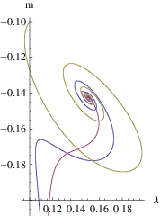
Diagonalizing we find that the linearized flow is governed by a pair of complex conjugate critical exponents with and , as well as a positive real one, . The nonzero imaginary part implies that the RG trajectories are spirals near the NGFP. As and are positive, the NGFP is UV-attractive in all three directions, i.e. all three scaling fields are relevant. The right eigenvectors associated with the eigenvalues and are respectively,
| (4.16) |
We can rewrite eq. (4.13) as:
| (4.17) |
Here, and .
| (a) | (b) |
|---|---|
 |
 |
In Fig.1(a) we show a typical trajectory which spirals into the NGFP as . It was found by solving the full nonlinear system numerically. The figure 1(b) shows also the plane spanned by the vectors and at the NGFP. This plane coincides almost with the plane where the spirals form. Since is not coplanar to and , it shifts the trajectories away from the plane spanned by and .
Figure 2 shows the three projections of various numerical solutions of the system (3.18); their initial points are in the vicinity of the NGFP.
| (a) | (b) | (c) |
|---|---|---|
 |
 |
 |
Summarizing this analysis we can say that adding the -monomial to the CREH truncation has lead to a new relevant scaling field, thus increasing the dimensionality of the UV critical surface of the NGFP by one unit. Since this dimensionality is related to the degree of predictivity an asymptotically safe theory can have, we see that a proper understanding of the background dependence of is important also from this point of view.
4.4 The fixed points of the 5 dimensional flow
Next we discuss whether and how the GFP and NGFP of the subsystem generalize to fix points of all five flow equations (3.18).
Let us begin with the GFP in the subsystem. Inserting into the remaining RG equations (3.18d) and (3.18e) we obtain
| (4.18a) | ||||
| (4.18b) | ||||
with . These equations admit two fixed points. The first one, denoted “G-G-FP”, achieves by , the second one, “G-NG-FP”, by . Their respective locations are
| G-G-FP: | (4.19) | |||
| G-NG-FP: | (4.20) |
Here and in the following the first label “G” (or “NG”, later on) indicates whether results from (“Gaussian”) or from (“non-Gaussian”). Likewise the second “G” or “NG” means that is achieved via or , respectively.
Trying to extend the NGFP of the subsystem, we are led to consider
| (4.21a) | ||||
| (4.21b) | ||||
Using the explicit formula for one finds that these beta functions, too, possess two common zeros, one with , the other with :
| NG-G-FP: | (4.22) | |||
| NG-NG-FP: | (4.23) |
Here we abbreviated . Table 1 contains a summary of the four fixed points we found.
| Fixed Point | FP in the Subsystem | |||||||
|---|---|---|---|---|---|---|---|---|
| G-G-FP | GFP | 0 | 0 | 0 | 0 | 0 | 0 | 0 |
| G-NG-FP | GFP | 0 | 0 | 0 | 0 | |||
| NG-G-FP | NGFP | 39.3 | 0.151 | 0 | 0 | 5.93 | 0 | |
| NG-NG-FP | NGFP | 39.3 | 0.151 | -25.2 | -0.779 | 5.93 | 19.6 |
Thus we may conclude that in the generalized truncation with , too, the toy model of conformally reduced gravity possesses a non-trivial fixed point. Actually there are two of them now, the NG-G-FP and the NG-NG-FP, but they differ only in their and values which do not affect the dynamical metric. Leaving infrared issues aside, an asymptotic safety construction based upon either of these fixed points is conceivable. We consider this an encouraging result which suggests that also full fledged QEG should continue to have a NGFP when the truncation is generalized correspondingly.
While it is gratifying to see that the qualitative features of the flow, in particular near the fixed point, did not change, a superficial glance at the results might convey the impression of considerable quantitative changes. For instance, for the presumably universal quantity we obtained . This figure has to be compared to found in [25] with the simple CREH truncation. This change is quite large in the following sense. In full QEG, the variations of under changes of or of within the class of truncations were at the level only. However, we must emphasize that it was clear from the outset that the toy model is much less stable under variations of or of the truncation than the full fledged QEG [25, 26, 27]. And indeed, the changes of the critical exponents caused by the modification are not larger than the variations within the scheme, comparing the “kin” and “pot” versions of the CREH truncation [25], for example. It is plausible to expect that in full QEG the inclusion of the leading bimetric invariants has a smaller impact on the results. It is clear, though, that at a certain point the terms will be more important than a further refinement of the truncations in the -sector.
The changes of the fixed point data are mainly due to the misinterpretation of background terms in the action as dynamical ones which is unavoidable in a truncation. The present truncation instead has no comparable “contamination” of the -terms by -contributions.
In this context it is interesting to note that the couplings in the “purely background” sector have no reason to be numerically small compared to the others in the dynamical sector. As an extreme example, let us compare the two cosmological constants at the NG-NG-FP. There the prefactors of and , respectively, are and . Obviously the background term is about 10 times larger than the “genuine” one. The prefactors of the respective Einstein-Hilbert terms are of the same order of magnitude though.
4.5 Testing the reliability of the truncation
We mentioned already that the -equation (1.12) and likewise the -equation (2.13) in the toy model are exact relations, resulting from the same functional integral as the corresponding FRGE. Therefore exact solutions to the FRGE automatically satisfy those relations exactly, while approximate solutions of the FRGE, if they are to be considered reliable, must satisfy them within the same degree of precision as the flow equation. In this section we use (2.13), restricted to the potential, in order to assess the reliability of the five-parameter truncation used above. This relation is instantaneous with respect to the RG time, it does not couple different scales , and so it can be checked at a single point of theory space. In particular we can test how well it is satisfied at the five fixed points found above.
This analysis is somewhat technical and the details are relegated to Appendix B. Here we only summarize the main results.
Analyzing (2.13) together with the fixed point condition on the still infinite dimensional theory space of arbitrary dimensionless potentials we find that the fixed point potential at the Gaussian fixed point is a pure monomial, without any admixture. The non Gaussian fixed points instead have a strong, probably predominant - component in their potential . Its precise form depends on the details of the . For equal fields one has always .
Turning to the three-parameter potential ansatz which retains only the monomials , and , with coefficients , , and , respectively, we find that this truncation satisfies the -equation only if and are small compared to all other relevant scales, and if . This is a selection criterion for solutions of the projected FRGE. By picking appropriate initial conditions and possibly restricting the interval one certainly can find consistent segments of RG trajectories.
It is quite remarkable that the -equation alone (without the flow equation!) tells us that the genuine cosmological constant should be small in this truncation, and that its background counterpart has the notorious dependence, well known from summing zero point energies.
Finally, checking how well the 4 fixed points of Table 1 satisfy the -equation we find that the G-G-FP and the G-NG-FP satisfy it exactly. The NG-G-FP and the NG-NG-FP are not exactly consistent, but the errors are still surprisingly small (as compared to the large change of relative to its CREH value, say).
In summary we can say that the instantaneous -equation for the potential does not hint at any severe inconsistency of the truncation which would matter at the qualitative level. For the quantitative details we refer to Appendix B.
5 Summary and conclusion
Our discussion started from the principle of “background independence” which any satisfactory theory of quantum gravity should respect. This requirement can be met in two complementary ways: either one constructs the theory without using a background at all, or one does introduce some background, as a technical tool and for mathematical convenience, but shows that no prediction of the theory depends on it. Aiming at the quantization of gravity along the lines of asymptotic safety we employed the gravitational average action approach here. It implements the second one of the above options by introducing an unspecified background metric . In the computation of the average action this metric is kept completely arbitrary, and in fact it gets promoted to a second argument of , equally important as the dynamical metric .
In particular the background metric is essential when it comes to devising a covariant and “background independent” coarse graining scheme for the gravitational field itself. The FRGE describing the scale dependence of the average action necessarily operates on a theory space consisting of functionals which depend on two metrics. Therefore this approach to the quantization of gravity naturally has a certain bimetric character.
In the earlier applications of the FRGE approach [6]-[31] its bimetric nature had not yet been explored in concrete computations. If one denotes the average action with the gauge fixing and ghost terms pulled out by where, by definition, , then all truncations used so far set1616 16 Up to a wave function renormalization, at most. . Projecting the RG flow on alone in deducing the beta functions from the exact FRGE certain -contributions of the functional traces are interpreted as -contributions. Clearly one would like to estimate the error caused by this mis-attribution, which requires retaining -type terms in the truncation ansatz. A second motivation for doing this is that must be known in order to set up the effective field equations.
In full fledged QEG the computation of flows in bimetric truncations is a formidable task. For this reason we started in this paper the analysis of such truncations within the simpler setting of conformally reduced gravity, a toy model which shares many properties with QEG, at least at the level of the Einstein-Hilbert truncation.
After preparing the stage in Section 2, we introduced a special bimetric truncation for the conformally reduced model in Section 3. It involves two separate Einstein-Hilbert terms with constants, and , respectively, for two conformally flat metrics and , as well as a nonderivative mixed term . From the point of view of the dynamical field the truncation ansatz is essentially a standard scalar action, with coupling , and mass square . In Section 4 we discussed the RG flow which follows from this truncation ansatz when a coarse graining operator is used which complies with the principle of “background independence”. The main results can be summarized as follows.
(A) Identifying with a fixed flat background metric, i.e. setting const, the EAA is found to be exactly that of a standard scalar field theory. We recover, for instance, the well known logarithmic running of and quadratic running of .
(B) The background cosmological constant , i.e. the coefficient of , has a very fast RG running proportional to . We find that, in the EAA framework, the sum over zero point energies contributes to the running of , rather than to the scale dependence of the genuine cosmological constant , the coefficient of . As a result, according to the effective Einstein equations for finite , it does not cause spacetime to curve. This should be relevant to the cosmological constant problem.
(C) In the “background independent” version of the earlier calculations of beta functions in the toy model which do not disentangle and -contributions one sets or at a certain stage of the calculation. This turns the dependence of the regulator on the background metric into a dependence on the dynamical field : . The beta functions one obtains in this way are quite different from those of an ordinary scalar matter field on a non-dynamical flat Euclidean space; the latter beta functions are obtained using .
Since in the calculation which disentangles and -contributions the background metric is always kept unspecified, and neither put equal to nor to , the difference in the conceptual status of the “background independent” and the “rigid background” functions disappears completely.
In a certain sense, the new treatment combines both of the old calculations into one. In the enlarged theory space of the fully “background independent” setting, with , there are certain couplings whose RG running reflects what happens in the rigid background treatment; the logarithmic running of the true cosmological constant is an example. But there are also couplings which are of no interest in the matter theory context, the prime example being .
(D) In the generalized truncation we found nontrivial fixed points which suggest that the toy model is asymptotically safe. Quantitatively, the terms cause considerable changes of the fixed point parameters, though.
(E) Thanks to the simplicity of the toy model it was possible to evaluate the instantaneous -equation which governs the -dependence of the EAA, and to use it for checking the quality of the truncation used. Remarkably, this equation by itself, together with the specific truncation ansatz, is sufficient to predict that the genuine cosmological constant is very small, and that runs proportional to .
(F) Finally we mention an issue we have not discussed yet. In [28] the information contained in the limit of the EAA was used to construct a well defined regularized functional integral and a corresponding bare action for asymptotically safe theories. When applied to the conformally reduced Einstein-Hilbert truncation, without disentangling and , this construction yields a bare action with a potential, while the effective potential of the nontrivial fixed point is a simple term. Clearly it is somewhat unusual to find the Coleman-Weinberg potential , nonanalytic in , at the bare level. In Appendix C we show that also this somewhat strange phenomenon is an artifact of the truncations which do not disentangle and contributions. In a bimetric truncation, the term which gets added in going from the effective to the bare fixed point action is essentially , and not .
Our discussion of the bimetric truncations in conformally reduced gravity should have made it clear that it is certainly worthwhile, and in fact necessary to perform a similar analysis in full fledged QEG. Because of the better stability properties of the full theory it is plausible to expect that the impact of the terms is smaller than in the toy model though. Those superior stability properties of the full gravity theory are, at least partially, due to the fact that it contains two completely different types of interactions, both of which independently drive the formation of a NGFP: the self interactions of the helicity-2 field coming from the -term, and the vertices due to the cosmological constant term . The toy model retains only the latter type.
Including terms in full QEG will require a considerable technical effort, however. In particular new efficient strategies for the computation of functional traces must be developed for this purpose. It would also be interesting to reanalyze the nontrivial fixed points found in higher dimensional Yang-Mills theory theory [35, 61] and the nonlinear sigma model [62] in the light of the above results.
Acknowledgements: We would like to thank J. Pawlowski, R. Percacci, and O. Rosten for helpful discussions.
Appendix
Appendix A Derivation of the beta functions
In this appendix we derive the flow equation for an arbitrary bimetric potential , the partial differential equation (3.13), as well as the beta functions of the five-parameter truncation displayed in (3.18). The starting point of all calculations is (3.12) which we shall project in various ways. We restrict ourselves to the topology and set throughout. All final results in particular those given in the main part of the paper are for the optimized shape function [60].
A.1 The partial differential equation for
In order to “project out” the term from (3.12) we insert -independent configurations on both sides. In this case it is advantageous to evaluate the functional trace in the eigenbasis of . Since, for , the Laplacians and are related by , and , the resulting trace in eq.(3.12) is of the form which is simply with . Upon changing the variable of integration from to we find
| (A.1) |
This is as far as one can go for a generic function . In the following we shall employ the optimized shape function [60]
| (A.2) |
which has the advantage that the -integral in (A.1) can be performed in closed form. Using (A.2) in (A.1) a trivial calculation brings us to the final result given in eq.(3.13) of the main text.
A.2 Projecting on the 3-parameter potential
Next we investigate what happens when we restrict the functional form of to the 3-parameter ansatz (3.3) which contains the monomials , and only. Again we face the problem that the vector field which governs the RG flow on the big space of functions is not a priori tangent to the 3-dimensional subspace spanned by , and . To get a flow on the subspace, governed by a vector field tangent to it, a “projection” has to be devised.
In order to streamline the notation we set
| (A.3) |
so that the 3-parameter potential (3.3) assumes the form
| (A.4) |
If we insert (A.4) straightforwardly on both sides of the RG equation for , eq.(3.13), the result is
| (A.5) |
with the abbreviation
| (A.6) |
In order to find the scale derivatives of the 3 couplings we must analyze the various “corners” of the - plane separately; they allow for different approximations (expansions) of the function .
If we may expand in powers of , yielding
| (A.7) |
Obviously none of the of the terms appearing in this expansion matches those on the LHS of (A.5). The conclusion is that, within this truncation, the RHS of (A.5) is equivalent to zero so that the couplings nave no nontrivial running. (Note that upon returning to dimensionful parameters, and dividing them by the factor included in the ansatz (3.1), the “+2” and the “” disappear from the first bracket of (A.5); dimensionful parameters in have no -dependence therefore.)
Conversely, when we can expand in , with the result
| (A.8) |
We observe that the first 3 terms of the power series expansion in are precisely those retained in the truncation ansatz, and the higher order terms are negligible when . As a consequence, equating the coefficients of , and on both sides of (A.5) implies nontrivial RG equations:
| (A.9) |
After returning to the variables the relations (A.9) become exactly the equations (3.18b), (3.18c), and (3.18e) presented in the main text.
To summarize: Depending on whether is large or small the RG equations on the 3-dimensional truncation subspace assume different forms; they are given by, respectively, (A.9) and a set of similar equations with zero on their RHS. Loosely speaking, different 3-dimensional RG flows correspond to different “projections” of the flow on the larger theory space. Specifying a truncation involves not only picking a set of monomials retained in the ansatz, it also involves specifying a projection. Even after having fixed the functional form of , different regions of field space might still require different projections, that is, different beta functions, for a reliable approximation.
In the present paper we employ only the beta functions corresponding to the case of small . One of the reasons is that we would like to establish the connection between the gravity theory and a standard scalar theory. In the perturbative quantization of the latter one sets and makes a power series (or rather polynomial) ansatz for , leading to RG equations similar to (A.9). Another reason is that we would like to have a simple model capable of describing the phase of unbroken diffeomorphism invariance in which the expectation value of the metric can vanish. This corresponds to at fixed, finite , so that in this situation.
A.3 The anomalous dimension
Next we calculate the anomalous dimension for the 3 parameter form of . To obtain an explicit formula for we use eq.(3.12) for a constant background field, together with an -dependent . As we plan to perform the trace in the eigenbasis we also insert again:
| (A.10) |
Consistent with the truncation we must perform a derivative expansion of the trace, thereby retaining only the term which is of second order both in and the number of derivatives. As it turns out, this term is automatically independent of , as is the LHS of (A.10). Hence we have the same monomial on both sides and obtain a nonzero
Actually we do not have to redo the explicit derivative expansion here since almost the same trace as in (A.10) has been evaluated in earlier investigations of the toy model in ref.[25]. (See in particular the computation of and the Appendix A there.) The only modification is the term in the denominator which is easy to take care of. From the results of [25] we can easily read off the answer for the anomalous dimension:
| (A.11) |
Here and are threshold functions defined in [25]. They can be evaluated for any . For the optimized shape function they read
| (A.12) |
When we insert (A.12) into (A.11) we obtain the final result (3.19a) given in the main text.
A.4 The anomalous dimension
In order to compute the anomalous dimension related to we could in principle evaluate (3.12) for an -dependent and constant ; then only the term would contribute on the LHS. Actually it turns out that the trace to be evaluated simplifies if, instead, we insert two equal, nonconstant fields: . Then also the term contributes, but its prefactor is known already. For the 3 parameter potential this leads to:
| (A.13) |
On the LHS we used that for the conformally flat metric . To find we now perform a covariant derivative expansion of the trace in (A.13), retaining only the Einstein-Hilbert term. This trace depends on in a twofold way: via the Laplace-Beltrami operator pertaining to , , and via the curvature scalar . It is most convenient to take care of the first dependence by heat kernel methods [6] and to expand out the second explicitly. Actually a very similar calculation has already been performed in [25], albeit in a different context and with a different interpretation. (See in particular the derivation of in [25].) Performing obvious replacements the trace term of interest can be read off from the results in [25]:
| (A.14) |
The functions and are the same as in [25], but the term shifts their argument. For the optimized shape function we have explicitly
| (A.15) |
When we solve eq.(A.14) for we obtain precisely the formula (3.19b) given in the main text.
Appendix B Testing the reliability of the truncation
In this appendix we employ the equation (2.13) in order to assess the reliability of the truncation used in this paper. At the exact level, a RG trajectory which solves the FRGE is automatically a solution of the equation. When we perform approximations this is no longer the case, and the degree with which the latter equation is satisfied can be used to judge the quality of an approximate solution to the FRGE. In particular this can be done when the FRGE and the equation are projected onto some subspace.
For the general ansatz (3.1), a calculation similar to the derivation of shows that the equation implies for the dimensionful and dimensionles potential, respectively,
| (B.1) | ||||
| (B.2) |
These relations hold true for the optimized shape function. Obviously they have a similar structure as the truncated flow equation. They are instantaneous, however; they contain no derivative with respect to . In particular, for a trajectory with UV fixed point, eq.(B.2) is valid at , i.e. it constrains the fixed point potential .
B.1 Fixed point potentials at the general level
To the extent some approximate RG trajectory is (approximately) consistent with the projected FRGE and the equation, any linear combination of these two equations will also be approximately satisfied by this trajectory. For instance, we may combine (3.17) and (B.2) in such a way that the complicated term involving disappears:
| (B.3) |
The term in (B.3) stems from the factor on the RHS of the flow equation (3.17). It is due to the factor in the normalization of the , see eq.(2.12). This prefactor contributes a term to .
It is instructive to consider (B.3) at a fixed point, . At the GFP we have and . Hence (B.2) tells us that and (B.3) yields . Taken together these relations imply that
| (B.4) |
where is a constant (which can be fixed as in [26]). Note that the fixed point potential (B.4) depends only on the dynamical field , not on the background.
At a NGFP, instead, one has , and (B.3) boils down to
| (B.5) |
This equation would imply that is a function of a single variable, . However, there exists no exact fixed point solution to the flow equation (3.17) of the form . This reflects the fact that we are dealing with approximate equations, and for consistency must be content with potentials which solve these equations only approximately.
Nevertheless the qualitative conclusion we can draw from (B.5) is that, at a NGFP, the fixed point potential is likely to involve both the dynamical field and the background . Moreover, there is a clear trend for the background field to be predominant. In fact if we change the normalization of and replace in its prefactor by a constant, the term disappears from the flow equation and from (B.3). As a consequence, eq.(B.5) gets replaced by . This equation alone would then imply that is a function of alone! Clearly, as we said above, we are dealing with approximate solutions to approximate equations so that this result cannot be taken at face value. But still it highlights the importance of the background field for the structure of the fixed point action.
B.2 The 3-parameter potential ansatz
Now we perform a further projection of the equation (B.1) namely on potentials of the form (3.3). It is then found to imply
| (B.6) |
Again, these conditions should not be taken at face value, but a reliable solution of the projected FRGE should satisfy them approximately. Hence the basic message of (B.6) is clear: The -parameter potential ansatz which retains only the monomials , and can be consistent only when the genuine cosmological constant is small compared to all other relevant scales and its background counterpart scales as .
It is quite remarkable that the equation alone is sufficient to predict that when , the result which obtains by summing zero point energies.
It is perhaps even more interesting and possibly relevant to the cosmological constant problem that the very structure of the potential ansatz, and therefore of the (conformally reduced) Einstein-Hilbert action in particular, favors a vanishing or at most small cosmological constant .
The conditions (B.6) read in dimensionless form
| (B.7) |
We interpret the first two of them as the requirement that and should be much smaller than unity, or at least significantly smaller than other typical couplings.
B.3 The fixed points from the 3-parameter potential
Finally we check to what extent the four fixed points of the system in Table 1 are in accord with (B.7). One finds that the G-G-FP and the G-NG-FP satisfy (B.7) exactly.
The NG-G-FP has the coordinates
Obviously and are “anomalously small” at this fixed point (compared to , say) and in particular much smaller that unity. This is indeed what (B.7) requires, and its third relation is satisfied exactly even.
The coordinates of the NG-NG-FP are
The and values are the same as above, and from and we get . According to the last relation of (B.7) this ratio should be equal to . Our result is off by a factor of . We interpret this number which is still remarkably close to unity as an indication that our treatment of the NG-NG-FP is at least qualitatively correct, and that this fixed point is presumably not an artifact of the truncation.
Appendix C From the effective to the
bare fixed point action
The limit of the EAA is closely related to the bare action which appears in the integrand of the underlying functional integral. In ref.[28] we explained how, after having introduced an UV regulator at scale1717 17 There should be no confusion between the UV cutoff and the cosmological constant. into the integral, the corresponding bare action relates to if one requires that the integral with reproduces the prescribed EAA in the limit . Under certain conditions a fixed point at the effective level implies a fixed point for the bare action, and one can derive an explicit functional differential equation for in dependence on . For the specific UV regulator used in [28] (“finite mode” regularization) it reads
| (C.1) |
Here stands for evaluated at , and denotes the Hessian of with respect to . Given for , eq.(C.1) may be used to find in the limit . (See [28] for further details.)
In [28] we applied this algorithm to conformally reduced gravity, making a local potential ansatz, without extra dependence , for both and . The former action contains the familiar dimensionless potential , the one in the latter is denoted . For the topology the effective NGFP potential turned out to be a pure monomial, , while the corresponding bare fixed point potential was much more complicate, behaving for asymptotically as
| (C.2) |
where is the bare Newton constant in . While this potential is of the familiar Coleman-Weinberg from, it is remarkable that here it appears as part of the bare action corresponding to a simple monomial in the effective one. Thus, compared to a standard scalar matter field theory, the situation is exactly inverted. Since a bare action nonanalytic in the field is a somewhat unusual situation it is worthwhile to reconsider this issue with a bimetric truncation.
As we explained in Appendix B, we cannot exclude the possibility that in a bimetric truncation the potential in is a complicated, possibly nonanalytic function of both and . However, we can exclude the possibility that the mere transition from the effective to the bare level generates Coleman-Weinberg like nonanalytic terms.
To see this in the simplest setting possible we make an ansatz for in which the potential does have an extra dependence but not the kinetic term:
| (C.3) |
For the bare action we make an analogous ansatz, with a bare Newton constant and a potential :
| (C.4) |
Now it is straightforward to insert (C.3), at , and (C.4) into (C.1) and to project out the nonderivative terms. In terms of the dimensionless quantities (3.14), (3.15), and analogously defined bare ones the result reads
| (C.5) |
This is a complicated differential equation for when is a given solution of the FRGE, evaluated at . For it relates the fixed point potentials and .
Eq.(C.5) is strikingly different from its analog in the earlier calculation where the and contributions were not disentangled. There we found:
| (C.6) |
Obviously the explicit ’s on the RHS of (C.5) are misinterpreted as ’s in the simpler truncation leading to (C.6). The Coleman-Weinberg potential (C.1) is a direct consequence of this misinterpretation. At the NGFP the effective potential is for which one can easily show that (C.6) has the asymptotic solution (C.1).
For the ”correct” equation (C.5) the situation is different: If is analytic in , so is the bare potential . In this case the RHS of (C.5) has the structure . Since, as always, , this expression admits a power series expansion in . So we see that when the effective fixed point potential is a power series in , the bare potential is a power series, too.
References
- [1]
For general introductions see C. Kiefer, Quantum Gravity, Second Edition,
Oxford Science Publications, Oxford (2007); H. Hamber, Quantum Gravitation, Springer, Berlin (2008). - [2]
A. Ashtekar, Lectures on non-perturbative canonical gravity,
World Scientific, Singapore (1991);
A. Ashtekar and J. Lewandowski, Class. Quant. Grav. 21 (2004) R53. - [3] C. Rovelli, Quantum Gravity, Cambridge University Press, Cambridge (2004).
- [4]
Th. Thiemann, Modern Canonical Quantum General Relativity,
Cambridge University Press, Cambridge (2007). - [5]
S. Weinberg
in General Relativity, an Einstein Centenary Survey,
S.W. Hawking and W. Israel (Eds.), Cambridge University Press (1979);
S. Weinberg, arXiv:0903.0568 [hep-th]. - [6] M. Reuter, Phys. Rev. D 57 (1998) 971 and hep-th/9605030.
- [7] D. Dou and R. Percacci, Class. Quant. Grav. 15 (1998) 3449.
- [8] O. Lauscher and M. Reuter, Phys. Rev. D 65 (2002) 025013 and hep-th/0108040.
- [9] M. Reuter and F. Saueressig, Phys. Rev. D 65 (2002) 065016 and hep-th/0110054.
- [10] O. Lauscher and M. Reuter, Phys. Rev. D 66 (2002) 025026 and hep-th/0205062.
- [11] O. Lauscher and M. Reuter, Class. Quant. Grav.19 (2002) 483 and hep-th/0110021.
- [12] O. Lauscher and M. Reuter, Int.J. Mod. Phys.A 17 (2002) 993 and hep-th/0112089.
- [13] W. Souma, Prog. Theor. Phys. 102 (1999) 181.
- [14] M. Reuter and F. Saueressig, Phys. Rev. D 66 (2002) 125001 and hep-th/0206145; Fortschr. Phys. 52 (2004) 650 and hep-th/0311056.
- [15] A. Bonanno and M. Reuter, JHEP 02 (2005) 035 and hep-th/0410191.
- [16]
For reviews see:
M. Reuter and F. Saueressig, arXiv:0708.1317 [hep-th];
O. Lauscher and M. Reuter in Quantum Gravity, B. Fauser,
J. Tolksdorf and E. Zeidler (Eds.), Birkhäuser, Basel (2007) and hep-th/0511260;
O. Lauscher and M. Reuter in Approaches to Fundamental Physics,
I.-O. Stamatescu and E. Seiler (Eds.), Springer, Berlin (2007). - [17]
R. Percacci and D. Perini,
Phys. Rev. D 67 (2003) 081503;
Phys. Rev. D 68 (2003) 044018; Class. Quant. Grav.21 (2004) 5035. - [18]
A. Codello and R. Percacci,
Phys. Rev. Lett.97 (2006) 221301;
A. Codello, R. Percacci and C. Rahmede, Int.J. Mod. Phys.A23 (2008); preprint arXiv:0805.2909 [hep-th]. - [19]
D. Litim,
Phys. Rev. Lett.92 (2004) 201301;
AIP Conf.Proc.841 (2006) 322;
P. Fischer and D. Litim, Phys. Lett. B 638 (2006) 497;
AIP Conf.Proc.861 (2006) 336. - [20] P. Machado and F. Saueressig, Phys. Rev. D 77 (2008) 124045.
- [21] D. Benedetti, P. Machado and F. Saueressig, preprint arXiv:0901.2984 [hep-th] and preprint arXiv:0902.4630 [hep-th].
- [22] O. Lauscher and M. Reuter, JHEP 10 (2005) 050 and hep-th/0508202.
- [23] M. Reuter and J.-M. Schwindt, JHEP 01 (2006) 070 and hep-th/0511021.
- [24] M. Reuter and J.-M. Schwindt, JHEP 01 (2007) 049 and hep-th/0611294.
- [25] M. Reuter and H. Weyer, Phys. Rev. D 79 (2009) 105005 and arXiv:0801.3287 [hep-th]; Gen. Rel. Grav. 41 (2009) 983 and arXiv:0903.2971 [hep-th].
- [26] M. Reuter and H. Weyer, Phys. Rev. D 80 (2009) 025001, and arXiv:0804.1475 [hep-th].
- [27] P. F. Machado and R. Percacci, arXiv:0904.2510 [hep-th].
- [28] E. Manrique and M. Reuter, Phys. Rev. D 79 (2009) 025008 and arXiv:0811.3888 [hep-th].
- [29] E. Manrique and M. Reuter, arXiv:0905.4220 [hep-th].
- [30] E. Manrique and M. Reuter, work in progress.
- [31] J.-E. Daum and M. Reuter, preprint arXiv:0806.3907 [hep-th].
- [32]
P. Forgács and M. Niedermaier,
hep-th/0207028;
M. Niedermaier, JHEP 12 (2002) 066; Nucl. Phys. B 673 (2003) 131;
Class. Quant. Grav.24 (2007) R171. - [33]
For detailed reviews of asymptotic safety in gravity see:
M. Niedermaier and M. Reuter, Living Reviews in Relativity 9 (2006) 5;
R. Percacci, arXiv:0709.3851 [hep-th]. - [34] C. Wetterich, Phys. Lett. B 301 (1993) 90.
- [35] M. Reuter, C. Wetterich, Nucl. Phys. B 417 (1994) 181.
- [36]
M. Reuter and C. Wetterich,
Nucl. Phys. B 427 (1994) 291,
Nucl. Phys. B 391 (1993) 147, Nucl. Phys. B 408 (1993) 91; M. Reuter, Phys. Rev. D 53 (1996) 4430, Mod.Phys. Lett. A 12 (1997) 2777. - [37] M. Reuter, C. Wetterich, Phys. Rev. D 56 (1997) 7893 and hep-th/9708051.
- [38] M. Reuter and C. Wetterich, Nucl. Phys. B 506 (1997) 483.
- [39]
J. Berges, N. Tetradis and C. Wetterich,
Phys.Rep.363 (2002) 223;
C. Wetterich, Int.J. Mod. Phys. A 16 (2001) 1951. - [40]
For reviews of the effective average action in Yang–Mills theory see:
M. Reuter, hep-th/9602012; J. Pawlowski, hep-th/0512261;
H. Gies, hep-ph/0611146. - [41]
H.W. Hamber, Gen. Rel. Grav. 41 (2009) 817 and arXiv:0901.0964 [gr-qc];
Phys. Rev. D 45 (1992) 507;
Phys. Rev. D 61 (2000) 124008; arXiv:0704.2895 [hep-th];
T. Regge and R.M. Williams, J.Math.Phys.41 (2000) 3964 and gr-qc/0012035. - [42] J. Ambjørn, J. Jurkiewicz and R. Loll, Phys. Rev. Lett.93 (2004) 131301.
- [43] J. Ambjørn, J. Jurkiewicz and R. Loll, Phys. Lett.B 607 (2005) 205.
- [44]
J. Ambjørn, J. Jurkiewicz and R. Loll,
Phys. Rev. Lett.95 (2005) 171301;
Phys. Rev. D 72 (2005) 064014; Contemp.Phys.47 (2006) 103. - [45]
L.F. Abbott,
Nucl. Phys. B 185 (1981) 189; Acta Phys. Polon. B 13 (1982) 33;
B.S. DeWitt, Phys.Rev.162 (1967) 1195;
M.T. Grisaru, P.van Nieuwenhuizen and C.C. Wu, Phys. Rev. D 12 (1975) 3203;
D.M. Capper, J.J. Dulwich and M. Ramon Medrano, Nucl. Phys. B 254 (1985) 737;
S.L. Adler, Rev.Mod.Phys.54 (1982) 729. - [46]
A. Bonanno and M. Reuter,
Phys. Rev. D 62 (2000) 043008 and hep-th/0002196;
Phys. Rev. D 73 (2006) 083005 and hep-th/0602159;
Phys. Rev. D 60 (1999) 084011 and gr-qc/9811026. - [47] M. Reuter and E. Tuiran, in Proceedings of the Eleventh Marcel Grossmann Meeting, H.Kleinert, R. Jantzen, R. Ruffini (Eds.), World Scientific, Singapore (2007) and hep-th/0612037.
- [48]
A. Bonanno and M. Reuter,
Phys. Rev. D 65 (2002) 043508 and hep-th/0106133;
M. Reuter and F. Saueressig, JCAP 09 (2005) 012 and hep-th/0507167. - [49]
A. Bonanno and M. Reuter,
Phys. Lett. B 527 (2002) 9 and astro-ph/0106468;
Int. J. Mod. Phys. D 13 (2004) 107 and astro-ph/0210472;
E. Bentivegna, A. Bonanno and M. Reuter, JCAP 01 (2004) 001
and astro-ph/0303150. - [50]
A. Bonanno and M. Reuter,
JCAP 08 (2007) 024 and arXiv:0706.0174 [hep-th];
J. Phys. Conf. Ser. 140 (2008) 012008 and arXiv:0803.2546 [astro-ph]. - [51]
A. Bonanno, G. Esposito and C. Rubano,
Gen. Rel. Grav. 35 (2003) 1899;
Class. Quant. Grav. 21 (2004) 5005;
A. Bonanno, G. Esposito, C. Rubano and P. Scudellaro,
Class. Quant. Grav. 23 (2006) 3103 and 24 (2007) 1443. - [52] M. Reuter and H. Weyer, Phys. Rev. D 69 (2004) 104022 and hep-th/0311196.
- [53] M. Reuter and H. Weyer, Phys. Rev. D 70 (2004) 124028 and hep-th/0410117.
- [54] M. Reuter and H. Weyer, JCAP 12 (2004) 001 and hep-th/0410119.
- [55]
F. Girelli, S. Liberati, R. Percacci and C. Rahmede,
Class. Quant. Grav.24 (2007) 3995. - [56] D. Litim and T. Plehn, Phys. Rev. Lett.100 (2008)131301.
- [57]
J. Moffat,
JCAP 05 (2005) 2003;
J.R. Brownstein and J. Moffat, Astrophys. J. 636 (2006) 721;
Mon. Not. Roy.Astron. Soc. 367 (2006) 527. - [58]
R. Floreanini and R. Percacci,
Nucl. Phys. B 436 (1995) 141;
Phys. Rev. D 46 (1992) 1566. - [59] O. Lauscher, M. Reuter and C. Wetterich, Phys. Rev. D 62 (2000) 125021 and hep-th/0006099 .
- [60]
D. Litim,
Phys. Lett.B 486 (2000) 92;
Phys. Rev. D 64 (2001) 105007;
Int.J. Mod. Phys.A 16 (2001) 2081. - [61] H. Gies, Phys. Rev. D 68 (2003) 085015.
- [62] A. Codello and R. Percacci, arXiv:0810.0715 [hep-th].
- [63] D. Giulini in Approaches to Fundamental Physics, I.-O. Stamatescu and E. Seiler (Eds.), Springer, Berlin (2007).
- [64] N. Straumann in Approaches to Fundamental Physics, I.-O. Stamatescu and E. Seiler (Eds.), Springer, Berlin (2007).
- [65] S. Weinberg, Rev. Mod. Phys. 61 (1989).