Further Results on the Riemann Hypothesis for Angular Lattice Sums
Abstract
Lattice sums, Dirichlet functions, Riemann hypothesis We present further results on a class of sums which involve complex powers of the distance to points in a two-dimensional square lattice and trigonometric functions of their angle, supplementing those in a previous paper (McPhedran et al, 2008). We give a general expression which permits numerical evaluation of members of the class of sums to arbitrary order. We use this to illustrate numerically the properties of trajectories along which the real and imaginary parts of the sums are zero, and we show results for the first two of a particular set of angular sums which indicate their density of zeros on the critical line of the complex exponent is the same as that for the product of the Riemann zeta function and the Catalan beta function.
1 Introduction
This paper adds to results in McPhedran et al (2008) (hereafter referred to as I) on the properties of a class of sums over two-dimensional lattices involving trigonometric functions of the angle to points in the lattice, and a complex power of their distance from the lattice origin. There, it was shown that certain of these angular sums had zeros on the critical line , but could not have zeros in a neighbourhood of it.
We derive a general expression which is exponentially convergent and permits the rapid and accurate evaluation of the angular sums irrespective of the value of the complex parameter . We demonstrate the high-order convergence of this formula by using it to illustrate a limiting formula for a particular set of angular lattice sums. We go on to consider the properties of trajectories along which the real and imaginary parts of a class of angular sums are zero, and in particular we establish accurate approximations for these trajectories when lies well outside the critical strip . We give preliminary results on the distribution of zeros on the critical line of two angular sums, which suggest that to leading order they have the same density of zeros as the product of the Riemann zeta function and the Catalan beta function. In Appendices we comment on the functional equation satisfied by a class of angular sums, and the properties which link angular sums of order up to ten.
The analytic results presented here are supported by numerical results obtained using Mathematica 7.0.1. Formal proofs of certain key properties of the angular sums and the location of their zeros will be given here, while others will be presented in a companion paper.
There are two principal motivations for the study presented here. The first is that the very general expression for the class of angular lattice sums derived in Section 2, and their connections with other angular lattice sums shown in Appendix A, enables them to be used in physical applications requiring regularization of sums over a two dimensional square lattice. The class of summands which can be addressed is wide, as it consists of any function which has a Taylor series in integer powers of trigonometric functions of the lattice point angle in the plane, and any complex power of its distance from the origin. For example, any summand of the type often encountered in solid state physics combining a Bloch-type phase factor and a function of distance having a Taylor series could be so represented. The second is that we show the angular lattice sums to be connected with the product of the Riemann zeta function and the Catalan beta function in a very natural way- for example, it seems that the densities of their zeros on the critical line are the same to leading orders. In this way, these angular sums may provide a new way to forge a link between the Riemann hypothesis and its generalization to other Dirichlet functions, as well as providing a wide class of functions, in which identified members obey a priori the hypothesis, and others do not. There are interesting parallels between this work and that of S. Gonek (2007), although we deal with double sums and Gonek with single sums.
2 An absolutely-convergent expression for angular lattice sums
We recall the definition from (I) of two sets of angular lattice sums for the square array:
| (1) |
where , and the prime denotes the exclusion of the point at the origin. The sum independent of the angle was evaluated by Lorenz (1871) and Hardy(1920) in terms of the product of Dirichlet functions:
| (2) |
Here is more commonly referred to as the Riemann zeta function, and as the Catalan beta function. A useful account of the properties of Dirichlet functions has been given by Zucker & Robertson (1976).
It is convenient to use a subset of the angular sums (1) as a basis for numerical evaluations. We note that the sums are zero if is odd. We next derive the following relationship for the non-zero sums :
| (3) |
where denotes the modified Bessel function of the second kind, or Macdonald function, with order and argument . The general form (3) may be derived following Kober (1936) in the usual way: a Mellin transform is used to give
| (4) |
The Poisson summation formula is then used to transform the sum over , giving
| (5) |
We then separate the axial contribution, which for comes from alone, and use Hobson’s integral
| (6) |
on the remaining double sum. This leads directly to (3).
It should be noted that the double sum in (3) is exponentially convergent. Indeed, from relation 9.7.2 in Abramowitz and Stegun (1972), the large argument approximation for the Macdonald function of order is
| (7) |
This means that the double sum starts to converge rapidly as soon as the argument everywhere exceeds the modulus of the order . In practice, accurate answers are achieved when sums are carried out over and from 1 to , where (the precise value of required being fixed by studies of the effect of increasing on the stability of the result). The representation (3) and finite combinations of it thus furnish absolutely convergent representations of trigonometric sums from the family (1) and close relatives, for any values of with finite modulus. These representations are easily represented numerically in any computational system incorporating routines for the Riemann zeta function of complex argument, and Macdonald functions of complex order and real argument. (In practice, the Macdonald function evaluations are most time-expensive in the region of values where has comparable magnitude to . Thus, it is efficient to create a table of these values for varying with , running up to an argument where the Macdonald function is less than an appropriate tolerance times its value for .)
As an example of the numerical efficacy of (1), we consider its use in illustrating a limiting property of the sums .We have
| (8) |
and as we require for a contribution, i.e.
| (9) |
The relationship (9) is illustrated numerically in Fig. 1. For the right-hand side of (9) to be accurate, the required order increases with , although convergence is also slow for near zero.


Another angular sum of great importance in this paper can easily be expanded in terms of the :
| (10) |
or, in terms of the Chebyshev polynomial of the first kind (Abramowitz & Stegun (1972), Chapter 22),
| (11) |
As the coefficients of this Chebyshev polynomial are explicitly known, the representation (11) enables any sum to be expressed as a linear combination of sums with .
The connections between various angular lattice sums grouped in systems with order up to 10 are explored in Appendix A.
3 Some properties of trigonometric lattice sums
The functional equation is known (see McPhedran et al. (2004), eqs. 32 and 59) for :
| (12) |
This equation also holds for , where it gives the functional equation for the product . It is in fact the dependence of the functional equation (12) which enables the derivation of many of the results in (I) and the present paper. As the derivation in McPhedran et al (2004) uses different notation to that in subsequent papers and here, we give a brief discussion of the argument leading to (12) in Appendix B.
This dependence in (12) is represented in two related functions:
| (13) |
where is in general complex. Note that is the ratio of two polynomials of degree , with one obtained from the other by replacing by :
| (14) |
We then introduce two sets of rescaled lattice sums:
| (15) |
and
| (16) |
Note that this definition means and have branch cuts where is real and negative. For example, for , the branch cut includes a circle in the plane (), with centre and radius .
An analytic function which combines lattice sums is defined by
| (17) |
It obeys the functional equation
| (18) |
and on the critical line ,
| (19) |
and
| (20) |
We note from (19) that
| (21) |
using the notation , a real-valued function. We can take the derivative with respect to of (21), to obtain:
| (22) |
We use the Cauchy-Riemann equations in (22), to obtain
| (23) |
and
| (24) |
The equation (23) indicates that, at points where contours of intersect the critical line, their tangent vector is given by , provided . (This requirement is that the left-hand side of (23) can be interpreted as the scalar product of the tangent vector and the gradient of , with the latter having a well-defined direction.) The equation (24) indicates that the tangent vectors for the contours of at the critical line are given by ,i.e. they are at right angles to those for the real part.
We note that, for , or, more strictly, for ,
| (25) |
Thus, for , (23) takes the approximate form
| (26) |
This shows that, as increases, the contours of strike the critical line at ever flatter angles (although the angle increases as increases). The direction of the intersection with the critical line is unique for every point where . Similar remarks apply to , where the equivalue contours cut the critical line at a direction given by the tangent vector , and thus their gradient at the point of intersection increases with .
4 Equivalue contours of and


In Figs. 2-4 we show contours on which the real and imaginary parts of are zero. Fig. 2 gives some detail of the region near for , and a further more detailed region on an undistorted geometric scale (including the semi-circle on which is real). Fig. 3 gives a more global view of null contours for ranging up to 20. Fig. 4 gives the detail of the null contours for near two values at which contours nearly touch. We introduce the notation for a zero on of , for a zero of and for a zero of . Then the zeros evident in Fig.3 are categorized as: .
The null contours have a number of interesting properties. Firstly, we can see that contours for the real part do indeed strike the critical line at a small angle to the axis, which decreases as increases, while the contours for the imaginary part strike the critical line almost vertically. Secondly, the contours for the real and imaginary parts intersect the critical line simultaneously, except for one point. This is at , where, as remarked in (I), , which permits to be zero, while is non-zero (see (19)).


We can see four null contours for the real part and five null contours for the imaginary part intersecting the axis . If we use the expression
| (27) |
we find that has a second order pole at , and first order poles at and . Numerical investigations show that near these points
| (28) |
and
| (29) |
We note that has zeros at the two first-order poles, where the trajectories approach the poles broadside (i.e., parallel to the axis), and two null trajectories approaching the second-order pole at and to the axis. has a zero at the second-order pole, where the null trajectory approaches broadside. The other null trajectory crossings of the real axis occur at 0.29782, 1.67735, -2.65568 and 4.21422. The last two of these are associated with minima of .

We show in Fig. 5 the behaviour of the null contours for large enough () to enable us to accurately approximate trigonometric sums by their first few terms:
| (30) |
so that
| (31) |
For beyond 4.21422, we see from Fig. 5 that neither the null trajectories of the real part or the imaginary part of can attain the real axis. In Fig. 6, we show for comparison the null trajectories associated with the prefactor term in square brackets in (31). It is evident from a comparison of Figs. 5 and 6 that the null trajectories are given accurately by the prefactor in the range of shown. Using Stirling’s formula (Abramowitz and Stegun (1972)), we can place the prefactor in exponential form for large, and find the constraint for null trajectories to be
| (32) |
where on the right-hand side the first value is for real-part zeros, and the second for imaginary-part zeros ( being an integer). From (32) we find that the equivalue contours alternate for large, with null contours for the real part sandwiched between those for the imaginary part, and vice versa (with each trajectory corresponding to a first-order zero). Each contour tends to zero as as .

Note that we may use the equation (18) to deduce relations governing the phase of . Dividing (18) by its conjugated form, we obtain
| (33) |
This agrees with (19) and (21) when . Furthermore, on the right-hand side of Fig. 3 we know that increases monotonically with , from its value of zero on the real axis. This enables us to assign values of the constant phase of the null contours there: , , , , , etc. Using (33) and (25), we see that the monotonic increase of with on the right in Fig. 3) forces a monotonic decrease of with on the left. We can then assign the phase values of the null contours there, again starting from zero on the real axis: , , , , , etc.
We can use this information to understand the behaviour of the null contours shown in Fig. 3. As the null contours of pass through a simple zero, their phase must change by , from to , or vice versa. However, we note that the relevant contours on the left in Fig. 3 which are almost symmetric to those on the right have opposite phase values. This means the null contours of vary smoothly as they cross the critical line. For the null contours of the situation is different: the phase change of forces them to avoid their almost symmetric counterpart on the left and ”jump up” a contour as they pass through a zero on the critical line. These remarks are in accord with the derivative estimates at the critical line (see equation (26) and subsequent discussion).
5 Some properties of zeros
The properties of the angular sums given in the preceding sections enable simple proofs to be given of some properties concerning the location of zeros of angular lattice sums. These properties form an interesting counterpoint to those of the zeros of Epstein zeta functions (see Bogomolny and Lebouef (1994) and references [26-30] of that paper). The Epstein zeta functions are characterized as having an infinite number of zeros lying on the critical line, but with many zeros lying off that line and with almost all zeros lying on the critical line or in its immediate neighbourhood. We have already seen in the example of Section 2 that this third property of Epstein zeta function zeros is not shared by those of the trigonometric double sum for large .
Theorem 5.1.
The trigonometric sums and have no zeros for on the critical line in the asymptotic region which are not zeros of both, and these will then be simultaneous zeros of and .
Proof 5.2.
We combine equations (15) and (16), to obtain
| (34) |
As the term in square brackets is real on the critical line, from the functional equation (12), we see that
| (35) |
The second term on the right-hand side of (35) is chosen according to the sign of the term in square brackets in (34). We can also use (20) to deduce that
| (36) |
Note that the term on the right-hand side in (36) incorporates the phase of the real function on the left-hand side, and is not necessarily the same as the second term on the right-hand side of (35).
We now consider the phases of and , particularly in the neighbourhood of zeros or . For brevity, we will adopt the following notations:
| (37) |
and
| (38) |
Then on the critical line, we have for and that
| (39) |
and
| (40) |
Using (39) and (40), we can rewrite (35) as
| (41) |
With a prime denoting derivatives, we obtain by differentiating (41)
| (42) |
We now consider the values of , and their derivatives in the neighbourhood of zeros of or , which are not zeros of both functions. Close to a zero of , we require
| (43) |
where , at the zero by Theorem 5.1. Using the last of (43) in (41) and (42), we find at the zero of that
| (44) |
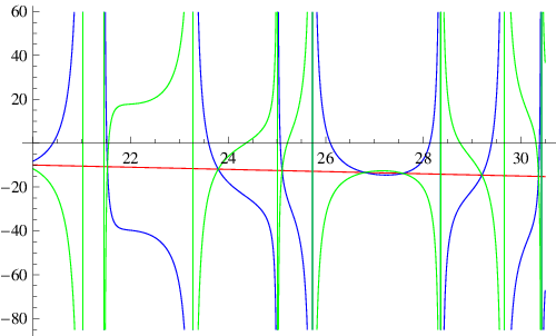
The relationships are exemplified in Fig. 7, where the variations with of the functions and are shown for the case . Note that, in terms of these, the relationship (41) controlling the variation of on the critical line is
| (47) |
Then, from (44), the zeros of are evident where the curves giving and intersect, which they do on the line giving the variation of . The curves of and also go off to infinity at zeros of , with their movement being in opposite directions in accord with (47). In Fig. 7 we see examples of there being none, one or two zeros between successive zeros of .

The next result relates to the independence of the functions on the critical line, again in the asymptotic region.
Theorem 5.3.
If is on the critical line in the asymptotic region and , are non-zero reals, then
| (48) |
If is on the critical line in the asymptotic region and , are non-zero reals with , then
| (49) |
Proof 5.4.
We suppose
| (50) |
Then
| (51) |
for an integer.
Corollary 5.5.
The sums , and have no zeros on the critical line in the asymptotic region which are not zeros of both and .
Proof 5.6.
We can also simply establish a corresponding result for the derivative for on the critical line.
Theorem 5.7.
The derivative function has no zeros for in the asymptotic region which are not zeros of of multiple order.
Proof 5.8.
We recall the result (19) for :
| (59) |
where is a real-valued function. Taking the derivative of with respect to and separating into real and imaginary parts, we find
| (60) | |||||
For to be zero, we find from the imaginary part of (60) that
| (61) |
We use (61) in the real part of (60), and, assuming is non-singular and , we complement (61) with
| (62) |
Since both the assumptions we have just mentioned are true in the asymptotic region, we have proved the theorem.
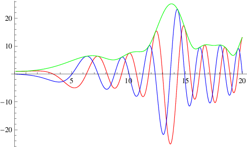
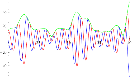
We provide plots of in Fig. 8. These show that the derivative is non-zero in the non-asymptotic region as well as in the asymptotic region. The numerical value of is 0.918604.
We next consider the properties of trajectories of constant phase which follow from the assumption that the Riemann Hypothesis holds for . As can be seen from Fig. 9, lines of constant phase between zeros of do not in general cross the critical line, but asymptote towards it, and their configuration is arranged about a zero of the derivative or equivalently of .


Theorem 5.9.
Given the Riemann hypothesis holds for , then lines of constant phase coming from can only cut the critical line at a zero of or of . Those lines of constant phase coming from cutting the critical line at a point which is not a zero of or of must curve back and pass through a zero of .
Proof 5.10.
The assumption of the Riemann hypothesis holding enables us to say that lines of constant phase coming from do not intersect before the critical line. Their phase monotonically decreases as increases in , while the phase of monotonically increases with . Thus, groups of constant phase lines coming in from cannot cut the critical line, except at a zero of . Isolated trajectories passing through points where are allowed. Such special trajectories separate lines of constant phase which curve up as and they move towards a zero of , from trajectories which curve down as .
Now consider sets of lines of constant phase approaching from the right. Their phase increases with , but if they were able to cross the line and progress towards it would have to decrease with . Thus they must turn and run alongside , with lines above the special trajectory curving up towards a zero of , and those below curving down towards a zero. Alternatively, they can cut the critical line at a point which is not a zero of or of . Such trajectories supply the lines of constant argument required for generic points on the critical line, and must return back to cut the critical line at a zero of . The region where they cross into is bounded on the left by a line of constant phase connecting a zero of with an adjacent zero of .
Note that the region where zeros of exist is confined to the neighbourhood of the critical line, since this partial derivative being zero corresponds to a horizontal segment on a line of constant phase (see, for example, Fig. 3). However, we may use the line of constant phase passing through the point on the critical line where as the separator between lines of constant phase going to the zero above this line from those going to the zero below (given the Riemann hypothesis is assumed to hold).
Theorem 5.11.
Given the Riemann hypothesis holds for , then there exists one and only one zero of on the critical line between two successive zeros of .
Proof 5.12.
We consider the analytic function
| (63) |
The real part of this function goes to at any zero of , and increases away from these logarithmic singularities. It must have at least one turning point between successive zeros. By the Cauchy-Riemann equations, such a turning point is a zero of .
Next, suppose there two or more zeros of between successive zeros and . Denote the upper two of such derivative zeros by and . As we have seen, each of these has constant phase lines coming from and passing through it, around which constant phase trajectories reverse their course. Those above curve up to as they approach the critical line, while those below it curve down. They cannot cross the constant phase line passing through , nor can they cross the critical line. They must then head back to , where they will breach the monotonic nature of the variation of with . Thus, this situation cannot arise.
We conclude this section with an investigation of the structure of lines of constant phase which cut the critical line and turn back to thereafter. We start with the expansion of around a point in the asymptotic region where , which is of the form:
| (64) | |||||
Here we have employed the asymptotic estimates for based on (25). The corresponding trajectories of constant phase may be shown to be rectangular hyperbolae, with their centre at
| (65) |
The second derivative factor in (65) is always negative, and tends to be much larger than the terms involving powers of . Thus, we see that the centre of the hyperbolic trajectories of constant phase will always lie to the left of the critical line, with its ordinate very close to . This displacement of the centre into creates the region in which phase lines can cut through and return to via passage through a zero of . Note that the centre corresponds to a point at which two lines of constant phase intersect; thus, it must have derivatives of phase along two independent lines which are zero. It therefore is a point at which both and are zero. From the Cauchy-Riemann equations, it also is a point at which and are zero- i.e., it is a point of extremum for both amplitude and phase.
These hyperbolic centre points are locations at which . The fact that they lie to the left of is is similar to the property proved by Speiser (1934) for .


The curves of constant phase of given in Fig. 10 illustrate some more of their general characteristics in the neighbourhood of zeros. For Fig. 10 (a), at the top of the figure, we see the centre of the hyperbolic phase curves; through this centre passes a curve on which . This curve connects the hyperbolic centre to the zero of below it, and also continues to the zero above; at each zero it is tangent to the axis. The curve marks points where the constant phase lines have vertical slope. The lowest line of constant phase on the right has vertical slope when it arrives at the zero of ; it corresponds to 3.04076, which is the value given by (19) for the phase on the critical line just above the zero. A second important line has the phase 3.04198, which is the phase corresponding to the centre of the hyperbola. This line again connects the hyperbolic centre to the zero. All lines whose phase lies between these values come in from the right, cross the zero line of , and curve back to pass through the zero of . Where they lie to the left of the zero line of , their phase increases as decreases; where they lie to the right, it increases as increases. Curves coming in from the left all pass through the zero without crossing the zero derivative line; their phase always increases as decreases.
For Fig. 10 (b), we show the phase contours below the zero, in the region down to the next zero. The phase at the centre of the hyperbolae is -0.1055, while the phase just above the bottom zero and just below the upper zero are respectively -0.107604 and -0.101134. Note the dashed line passing through the centre, along which . From the Cauchy-Riemann equations, this is perpendicular to the solid line defined by (a fact disguised by the different scales on the horizontal and vertical axes).
6 Distributions of zeros
We return to the left-hand side of expression (32), in which we replace by , and expand assuming , with large enough to ensure accuracy of (32). The result is
| (66) |
As for each increment of of this expression we get one null line of the real part of and one of the imaginary part, and these intersect at to give one zero there (assuming the Riemann hypothesis holds for ), we can divide (66) by , and regard the result as a distribution function for zeros of :
| (67) |
Now, from Titchmarsh and Heath-Brown (1987), the distribution function for the zeros of the Riemann zeta function on the critical line is
| (68) |
We complement this with the numerical estimate from McPhedran et al (2007) for the distribution function of the zeros of :
| (69) |
Adding (68) and (69) we obtain the distribution function for the zeros of (see (17)):
| (70) |
When we compare this with (67), and use the equation
| (71) |
it suggests the hypothesis that the distribution function of zeros of is the same as that of (70), to the number of terms quoted:
| (72) |
Strong numerical evidence supporting this is given in Table 1, which also shows zero counts for and . Note that the numbers of zeros found for , and are virtually the same. This rules out any variation with increasing order similar to that of Dirichlet functions, where increasing order results in significant increases in density of zeros (compare (69) and (68), or the second and third columns of Table 1).
Comparing the data of Table 1 with the discussion in Bogomolny and Lebouef (1994), we can see that the split up of into averaged parts given by expressions like (68-72) and oscillating parts applies to and to the . However, it would be value to extend the numerical investigations of Table 1 to much higher values of , to render the characterization of the oscillating term more accurate. Such an extension may require the development of an alternative algorithm to that based on (3), which will probably become unwieldy for values of of order .


In Fig. 11 we compare the distributions of the differences between zeros on the critical line for (left) and (right). The distributions are quite different, even with this modest data set. Bogomolny and Lebouef (1994) have studied the case of using 10,000 zeros after , and contrast the distribution for with that for each function separately. The separate factors in fact have distributions like that that for . The function compared with the histogram in the right of Fig. 11 corresponds to the Wigner surmise, which (Bogomolny and Lebouef, 1994, Dietz and Zyczkowski, 1991) for the unitary ensemble takes the form
| (73) |
Here the separation between zeros has been rescaled to have a mean of one. Bogomolny and Lebouef (1994) comment that the left distribution is that of an uncorrelated superposition of two unitary ensemble sets. Note as one indicator of this that there is not the same pronounced tendency for the probability to go to zero with separation on the left as on the right, where the distribution clearly comes from a single ensemble. Recall that Table 1 shows that the frequency distribution for zeros is the same for and . This makes the strong difference in the distributions of the gaps all the more interesting.
| 0-10 | 0 | 1 | 2 | 3 | 2 | 3 |
|---|---|---|---|---|---|---|
| 10-20 | 1 | 4 | 5 | 10 | 5 | 5 |
| 20-30 | 2 | 5 | 6 | 13 | 7 | 7 |
| 30-40 | 3 | 4 | 8 | 15 | 8 | 8 |
| 40-50 | 4 | 6 | 8 | 18 | 8 | 8 |
| 50-60 | 3 | 5 | 9 | 17 | 9 | 9 |
| 60-70 | 4 | 6 | 9 | 19 | 10 | 10 |
| 70-80 | 4 | 6 | 11 | 21 | 10 | 10 |
| 80-90 | 4 | 7 | 11 | 22 | 11 | 10 |
| 90-100 | 4 | 6 | 10 | 20 | 10 | 12 |
| 0-100 | 29 | 50 | 79 | 158 | 80 | 82 |
| (68),(69),(72) | 28 | 50 | 78 | 156 | ||
| 100-110 | 4 | 7 | 11 | 22 | 11 | 10 |
| 110-120 | 5 | 7 | 12 | 24 | 12 | 12 |
| 120-130 | 5 | 7 | 12 | 24 | 12 | 12 |
| 130-140 | 5 | 7 | 12 | 24 | 12 | 12 |
| 140-150 | 4 | 7 | 12 | 23 | 12 | 11 |
| 150-160 | 6 | 7 | 12 | 25 | 12 | 13 |
| 160-170 | 6 | 7 | 13 | 26 | 13 | 12 |
| 170-180 | 6 | 8 | 13 | 27 | 13 | 13 |
| 180-190 | 5 | 8 | 13 | 26 | 12 | 14 |
| 190-200 | 5 | 7 | 13 | 25 | 14 | 13 |
| 0-200 | 80 | 122 | 202 | 404 | 203 | 204 |
| (68),(69),(72) | 78 | 122 | 200 | 400 | ||
| 200-210 | 6 | 8 | 13 | 27 | 12 | 13 |
| 210-220 | 5 | 8 | 14 | 27 | 15 | 14 |
| 220-230 | 6 | 8 | 13 | 27 | 13 | 13 |
| 230-240 | 6 | 8 | 14 | 28 | 14 | 14 |
| 240-250 | 6 | 8 | 14 | 28 | 14 | 13 |
| 250-260 | 6 | 8 | 13 | 27 | 14 | 15 |
| 260-270 | 6 | 8 | 15 | 29 | 14 | 13 |
| 270-280 | 6 | 8 | 14 | 28 | 14 | 15 |
| 280-290 | 6 | 8 | 15 | 29 | 15 | 14 |
| 290-300 | 6 | 9 | 14 | 29 | 13 | 15 |
| 0-300 | 137 | 203 | 341 | 681 | 341 | 343 |
| (68),(69),(72) | 137 | 203 | 340 | 680 |
Acknowledgements.
The research of R.McP. on this project was supported by the Australian Research Council Discovery Grants Scheme.References
- [1] Abramowitz, M. & Stegun, I. A. 1972 Handbook of Mathematical Functions with Formulas, Graphs and Mathematical Tables. New York: Dover.
- [2] Bogomolny, E. & Lebouef, P. 1994 Statistical properties of the zeros of zeta functions- beyond the Riemann case. Nonlinearity 7 1155-1167.
- [4] Dietz, B. & Zyczkowski,K. 1991 Level-spacing distributions beyond the Wigner surmise. Z. Phys. B- Condensed Matter 84 157-158.
- [5] Gonek, S., 2007 Finite Euler Products and the Riemann Hypothesis arxiv:0704.3448
- [7] Hardy, G. H. 1920 On some definite integral considered by Mellin. Mess.Math. 49, 86-91.
- [9] Kober, H. 1936 Transformation formula of certain Bessel series, with reference to zeta functions Math. Zeitschrift 39, 609-624
- [11] Lorenz, L. 1871 Bidrag til talienes theori, Tidsskrift for Math. 1 , 97-114.
- [13] McPhedran, R. C., Smith, G. H., Nicorovici, N. A. & Botten, L. C. 2004 Distributive and analytic properties of lattice sums. J. Math. Phys. 45, 2560-2578.
- [15] McPhedran, R. C., Botten, L. C. & Nicorovici, N. A. 2007 Null trajectories for the symmetrized Hurwitz Zeta Function Proc. Roy. Soc. A 463 303-319
- [17] McPhedran, R.C., Zucker, I.J., Botten, L.C. & Nicorovici, N.A.. 2008 On the Riemann Property of Angular Lattice Sums and the One-Dimensional Limit of Two-Dimensional Lattice Sums. Proc. Roy. Soc. A, 464, 3327-3352.
- [19] Speiser, A., 1934 Geometrisches zur Riemannschen Zetafunktion. Math. Ann. 110, 514-521.
- [21] Titchmarsh, E. C. & Heath-Brown, D. R. 1987 The theory of the Riemann zeta function, Oxford: Science Publications.
- [23] Zucker, I.J. & Robertson, M.M.. 1976 Some properties of Dirichlet series. J. Phys. A. Math. Gen. 9 1207-1214
Supplementary Notes on Systems of Angular Sums
We give here results linking trigonometric lattice sums of order up to ten, which show that they may be generated from three independent sums, , , and . We also give expressions in terms of sums of Macdonald functions of the Kober-type from which these independent sums may be calculated.
A basic result we use relies on the symmetry of the square lattice:
| (74) |
from which we obtain
| (75) |
for any positive integer. We can also expand in terms of powers of , using the expressions for the Chebyshev polynomials in Table 22.3 of Abramowitz & Stegun (1972). This enables us to express in terms of with , and being a positive integer. In this way, we can inductively arrive at the results below.
.1 Order 0
The only sum of this type is , given by equation (2). It is given by a modified form of (3), since there are contributions from both axes , rather than just :
| (76) |
.2 Order 2
The single sum of order 2 is
.3 Order 4
.4 Order 6
.5 Order 8
Two other sums in this system are
| (87) |
and
| (88) |
Using the result (84), we have calculated curves showing the modulus of as a function of on the critical line. These are given in Figs. 12-13, and the distributions of zeros they show are given in Table 1.


.6 Recurrence Relations
We can generalize the above procedure by establishing recurrence relations for the trigonometric sums. We consider
| (89) |
Expanding using the Binomial Theorem, we obtain
| (90) |
If is even, (90) gives an identity:
| (91) |
while for odd we obtain an expression for in terms of lower order sums:
| (92) |
It may be checked that the two relations (91) and (92) give equivalent results in the cases given above.

In Fig. 14 we give null contours of the real part and imaginary part of , for comparison with those of in Fig. 3. It will be noted that there are now three lines giving the contours on which , and these are not circles (as was the single exemplar in Fig. 3). There is a corresponding increase in the number of null contours starting and finishing on the real axis, and in the value of at which the last one reaches the real axis. There are two examples in Fig. 14 of zeros on the critical line of the real part, but not the imaginary part (), and one of a zero of the imaginary part but not the real part (). The null contours starting at and ending at settle down to an asymptotic behaviour for somewhat larger values of than in Fig. 3, but are otherwise similar to the lower order null contours.
.7 Order 10
The new sum we use from (3) is , which, from (92), is
| (93) |
Other sums in the system are:
| (94) |
and
| (95) |
Derivation of the Functional Equation for
We start with the equation (30) from McPhedran et al (2004). This equation uses the Poisson summation formula to derive a connection between a sum over a direct lattice of points with polar coordinates , and a corresponding sum over the reciprocal lattice, where the lattice points are labelled . Considering the case of a square lattice with period , the reciprocal lattice points are . The sum in the direct lattice incorporates a phase term of the Bloch type, with wave vector , and the result of the Poisson formula is
| (96) |
Here the sum over the reciprocal lattice in fact runs over a set of displaced vectors:
| (97) |
where in (97) the second and third expressions are in rectangular and polar coordinates. Note that in (96) and (97), and run over all integer values, and gives the direction of .
We express the relation (96) in non-dimensionalized form, taking out a factor on the left-hand side, and a factor on the right-hand side. We put , and obtain
| (98) |
If we now let , set and take , we obtain the desired result:
| (99) |