Capacity of a Class of Linear Binary Field Multi-source Relay NetworksThanks: S.-W. Jeon and S.-Y. Chung are with the Department of EE, KAIST, Daejeon, South Korea (e-mail: swjeon@kaist.ac.kr; sychung@ee.kaist.ac.kr).Thanks: The material in this paper was presented in part at the Information Theory and Applications Workshop, University of California San Diego, La Jolla, CA, February 2009, and at the IEEE International Symposium on Information Theory (ISIT), Seoul, Korea, June/July 2009.

Sang-Woon Jeon Student Member IEEE Sae-Young Chung Senior Member IEEE Affiliation:

Abstract

Characterizing the capacity region of multi-source wireless relay networks is one of the fundamental issues in network information theory. The problem is, however, quite challenging due to inter-user interference when there exist multiple source–destination (S–D) pairs in the network. By focusing on a special class of networks, we show that the capacity can be found. Namely, we study a layered linear binary field network with time-varying channels, which is a simplified model reflecting broadcast, interference, and fading natures of wireless communications. We observe that fading can play an important role in mitigating inter-user interference effectively for both single-hop and multi-hop networks. We propose new encoding and relaying schemes with randomized channel pairing, which exploit such channel variations, and derive their achievable rates. By comparing them with the cut-set upper bound, the capacity region of single-hop networks and the sum capacity of multi-hop networks can be characterized for some classes of channel distributions and network topologies. For these classes, we show that the capacity region or sum capacity can be interpreted as the max-flow min-cut theorem.

I Introduction

Capacity characterization of general wireless relay networks is a fundamental problem in network information theory. However, the capacity is not fully characterized even for the simplest network consisting of single source, single relay, and single destination [1]. In wireless environments, a transmit signal will be heard by multiple nodes, which we call the broadcast nature of wireless communications, and a receiver will receive the superposition of simultaneously transmitted signals from multiple nodes, which we call the interference nature of wireless communications. Furthermore wireless channels may be time-varying due to fading, and there is noise at each receiver. Considering all these makes the problem vary hard.

Hence, one of the promising approaches is to study simplified relay networks, whose results can provide insights towards exact or approximate capacity characterization for more general wireless relay networks. Let us first look at some cases for which the capacity is known. For wireline relay networks, routing is enough to achieve the unicast capacity [2]. On the other hand, routing alone cannot achieve the multicast capacity and network coding has been shown to be optimal in this case [3, 4, 5, 6]. For deterministic relay networks with no interference, the unicast capacity has been characterized in [7] and the extension to the multicast case has been studied in [8]. The multicast capacity of erasure networks with no interference has been also characterized in [9]. When there is no broadcast, the unicast capacity of erasure networks has been characterized in [10], which is the dual network studied in [9]. For all these mentioned networks, the unicast or multicast capacity can be interpreted as the max-flow min-cut theorem.

Notice that although such orthogonal transmission or reception is possible in practice by using time, frequency, or code-division techniques, it is suboptimal in general. Therefore, simplification of wireless relay networks while preserving both broadcast and interference natures is crucially important to capture the essence of wireless communications. One of the simplest models that successfully reflect both broadcast and interference natures is a linear finite field relay network [11, 12, 13], where a node transmits an element in the finite field and receives the sum of transmit signals in the same finite field. Recently, the work in [13] has shown that the max-flow min-cut theorem also holds for deterministic linear finite field relay networks. After the capacity characterization of linear finite field relay networks, the approximate capacity of Gaussian relay networks has been characterized within a constant number of bits/s/Hz using the quantize-random-map-and-forward by the same authors [14].

In spite of the surging importance of multi-source relay networks, capacity characterization is much more challenging if there exist multiple source–destination (S–D) pairs in a network. Even for linear finite field relay networks, the extension of the results in [13] to the multi-source does not seem to be straightforward. Notice that the main difficulty arises from the fact that the transmission of other sessions acts as inter-user interference and, as a result, the cut-set upper bound is not tight in general. Due to these difficulties, the existing capacity or approximate capacity results are limited in specific network topologies such as two-user interference channel [15, 16], many-to-one and one-to-many interference channel [17], two-way channel [18, 19], two-user two-hop relay network [20, 21], and double Z-channel [22]. Therefore, one of the basic questions is whether we can characterize the capacity or approximate capacity for more general network topologies or other classes of relay networks.

In this paper, we study a layered multi-source linear binary field relay network with time-varying channels, which captures three key characteristics of wireless environment, i.e., broadcast, interference, and fading. Note that a random coding strategy, which is still optimal in fading single-source networks [23, 24], does not work anymore for our network model due to the inter-user interference. As mentioned before, a fundamental issue in multi-source networks is how to manage inter-user interference properly. We observe that fading can play an important role in mitigating such interference efficiently, which leads to the capacity characterization for certain classes of networks. More specifically, for single-hop networks, inter-user interference can be removed completely at each destination by using two particular channel instances jointly. For multi-hop networks, by using a series of particular channel instances over multiple hops, each destination can also decode its message without interference.

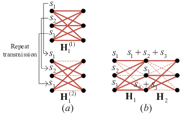
Refer to caption — Fig. 1: Interference mitigation for the single-hop network (a) and for the two-hop network (b), where the solid lines and the dashed lines denote the corresponding channels are ones and zeros, respectively.

As an example, consider the three-user linear binary field relay network in Fig. 1, where $s_{k}\in\mathbb{F}_{2}$ denotes the information bit of the $k$ -th source and the symbol in each node denotes the transmit signal of that node. For single-hop networks, as shown in Fig. 1. (a), by transmitting the same bit twice at each source through $\mathbf{H}^{(1)}_{1}$ and $\mathbf{H}^{(2)}_{1}$ such that $\mathbf{H}^{(1)}_{1}+\mathbf{H}^{(2)}_{1}=\mathbf{I}$ , each destination can cancel interference by adding the two received signals, where $\mathbf{H}^{(1)}_{1}$ and $\mathbf{H}^{(2)}_{1}$ denote the two different channel instances of the first hop and $\mathbf{I}$ denotes the identity matrix. Related works dealing with the inseparability of parallel interference channels can be found in [25, 26, 27, 28] and the references therein. The idea of opportunistically pairing two channel instances, i.e., $\mathbf{H}^{(1)}_{1}+\mathbf{H}^{(2)}_{1}=\mathbf{I}$ , also appeared in [27, 28]. This can be considered as a different and simpler way of doing interference alignment [29, 30]. For two-hop networks, as shown Fig. 1. (b), we notice that each destination can receive the information bit without interference if $\mathbf{H}_{2}\mathbf{H}_{1}=\mathbf{I}$ , where $\mathbf{H}_{1}$ and $\mathbf{H}_{2}$ denote the channel instances of the first and second hop, respectively. In general, the interference-free communication is possible for $M$ -hop networks, $M\geq 2$ , by opportunistically pairing the series of channel instances from $\mathbf{H}_{1}$ to $\mathbf{H}_{M}$ such that $\mathbf{H}_{M}\mathbf{H}_{M-1}\cdots\mathbf{H}_{1}=\mathbf{I}$ , where $\mathbf{H}_{m}$ denotes the channel instance of the $m$ -th hop.

Based on these key observations, we propose encoding and relaying schemes which make such opportunistic pairing of channel instances possible. By comparing their achievable rate regions with the cut-set upper bound, we characterize the capacity region of single-hop networks and the sum capacity of multi-hop networks for some classes of network topologies and channel distributions.

This paper is organized as follows. In Section II, we define the network model and state the multi-source relay problem and the notations used in the paper. In Section III, we derive the general cut-set upper bound, which will be used to prove the converses in Section IV. In Section IV, new encoding and relaying schemes are proposed to mitigate inter-user interference, which characterizes the capacity region or sum capacity for certain classes of networks. We conclude this paper in Section V and refer the proofs of the lemmas to Appendices I and II.

II System Model

In this section, we first explain the underlying network model and then define the achievable rate region and the notations used in the paper. Throughout the paper, $\mathbf{A}$ and $\mathbf{a}$ denote a matrix and a vector, respectively. The symbol $\mathcal{A}$ denotes a set and $|\mathcal{A}|$ denotes the cardinality of $\mathcal{A}$ .

II-A Linear Binary Field Relay Networks

We study a layered network in Fig. 2 that consists of $M+1$ layers having $K_{m}$ nodes at the $m$ -th layer, where $m\in\{1,\cdots,M+1\}$ . Let us denote $K_{\operatorname{max}}=\operatorname{max}_{m}\{K_{m}\}$ and $K_{\operatorname{min}}=\operatornamewithlimits{min}_{m}\{K_{m}\}$ . The $(k,m)$ -th node refers to the $k$ -th node at the $m$ -th layer. Then $K=K_{1}=K_{M+1}$ is the number of S–D pairs and the $(k,1)$ -th node and the $(k,M+1)$ -th node are the source and the destination of the $k$ -th S–D pair, respectively. Notice that if $M=1$ , the network becomes a $K$ -user interference channel.

Consider the $m$ -th hop transmission. The $(i,m)$ -th node and the $(j,m+1)$ -th node become the $i$ -th transmitter (Tx) and the $j$ -th receiver (Rx) of the $m$ -th hop, respectively, where $i\in\{1,\cdots,K_{m}\}$ and $j\in\{1,\cdots,K_{m+1}\}$ . Let $x_{i,m}[t]\in\mathbb{F}_{2}$ denote the transmit signal of the $(i,m)$ -th node at time $t$ and $y_{j,m}[t]\in\mathbb{F}_{2}$ denote the received signal of the $(j,m+1)$ -th node at time $t$ . Let $h_{j,i,m}[t]\in\mathbb{F}_{2}$ be the channel from the $(i,m)$ -th node to the $(j,m+1)$ -th node at time $t$ . The relation between the transmit and received signals is given by

y_{j,m}[t]=\sum_{i=1}^{K_{m}}h_{j,i,m}[t]x_{i,m}[t],

(1)

where all operations are performed over $\mathbb{F}_{2}$ ¹¹ 1 We focus on the binary field $\mathbb{F}_{2}$ in this paper, but some results can be directly extended to $\mathbb{F}_{q}$ (see Remarks 1 and 2).. We assume time-varying channels such that

\Pr(h_{j,i,m}[t]=1)=p_{j,i,m}

(2)

and $h_{j,i,m}[t]$ are independent of each other for different $i$ , $j$ , $m$ , and $t$ . This assumption can be generalized to block fading with coherence time of $T$ symbols, where $T\gg 1$ such that there is enough time for CSI to be spread to relevant nodes. We assume $T=1$ for notational simplicity since our result does not explicitly depend on $T$ as long as it is big enough such that CSI is available at all relevant nodes. Let $\mathbf{x}_{m}[t]$ and $\mathbf{y}_{m}[t]$ be the $K_{m}\times 1$ transmit signal vector and $K_{m+1}\times 1$ received signal vector of the $m$ -th hop, respectively, where $\mathbf{x}_{m}[t]=\left[x_{1,m}[t],\cdots,x_{K_{m},m}[t]\right]^{T}$ , $\mathbf{y}_{m}[t]=\left[y_{1,m}[t],\cdots,y_{K_{m+1},m}[t]\right]^{T}$ . Then the transmission of the $m$ -th hop can be represented as

\mathbf{y}_{m}[t]=\mathbf{H}_{m}[t]\mathbf{x}_{m}[t],

(3)

where $\mathbf{H}_{m}[t]$ is the $K_{m+1}\times K_{m}$ channel matrix of the $m$ -th hop having $h_{j,i,m}[t]$ as the $(j,i)$ -th element. We assume that both Txs and Rxs of the $m$ -th hop causally know the global channel state information (CSI) up to the $m$ -th hop. That is, at time $t_{0}$ , the nodes in the $m$ -th layer know $\{\mathbf{H}_{1}[t],\cdots,\mathbf{H}_{m}[t]\}_{t=1}^{t_{0}}$ if $m\leq M$ and $\{\mathbf{H}_{1}[t],\cdots,\mathbf{H}_{M}[t]\}_{t=1}^{t_{0}}$ if $m=M+1$ .

For a broad class of networks, if the channel dimension of a certain hop is smaller than those of the other hops, then the average channel rank of the hop is likely to be less than those of the other hops. The following definition formally states this class of networks.

Definition 1

Let $m_{0}=\operatorname{arg}\operatornamewithlimits{min}_{m\in\{1,\cdots,M\}}\mathbb{E}(\operatorname{rank}(\mathbf{H}_{m}[1]))$ ²² 2 Notice that $\mathbb{E}(\operatorname{rank}(\mathbf{H}_{m}[t]))$ is the same for all $t$ .. A linear binary relay network is said to have a minimum-dimensional bottleneck-hop $m_{0}$ if $K_{m}\geq K_{m_{0}}$ and $K_{m+1}\geq K_{m_{0}+1}$ or $K_{m}\geq K_{m_{0}+1}$ and $K_{m+1}\geq K_{m_{0}}$ for all $m\in\{1,\cdots,M\}$ .

In this paper, we will study the class of networks satisfying Definition 1. Notice that any networks with $K_{m}=K$ for all $m\in\{1,\cdots,M+1\}$ or any one-hop or two-hop networks are included in this class of networks regardless of channel distributions.

II-B Problem Statement

Based on the previous network model, we define a set of length- $n$ block codes. Let $W_{k}$ be the message of the $k$ -th source uniformly distributed over $\{1,2,\cdots,2^{nR_{k}}\}$ , where $R_{k}$ is the rate of the $k$ -th source. For simplicity, we assume $nR_{k}$ is an integer. Then a $\left(2^{nR_{1}},\cdots,2^{nR_{K}};n\right)$ code consists of the following encoding, relaying, and decoding functions.

•

(Encoding)

For $k\in\{1,\cdots,K\}$ , the set of encoding functions of the $k$ -th source is given by $\{f_{k,1,t}\}_{t=1}^{n}:\{1,\cdots,2^{nR_{k}}\}\to\mathbb{F}_{2}^{n}$ such that

$x_{k,1}[t]=f_{k,1,t}(W_{k})\mbox{ for }t\in\{1,\cdots,n\}.$ (4)
•

(Relaying)

For $m\in\{2,\cdots,M\}$ and $k\in\{1,\cdots,K_{m}\}$ , the set of relaying functions of the $(k,m)$ -th node is given by $\{f_{k,m,t}\}_{t=1}^{n}:\mathbb{F}_{2}^{n}\to\mathbb{F}_{2}^{n}$ such that

$x_{k,m}[t]=f_{k,m,t}\left(y_{k,m-1}[1],\cdots,y_{k,m-1}[t-1]\right)\mbox{ for }t\in\{1,\cdots,n\}.$ (5)
•

(Decoding)

For $k\in\{1,\cdots,K\}$ , the decoding function of the $k$ -th destination is given by $g_{k}:\mathbb{F}_{2}^{n}\to\{1,\cdots,2^{nR_{k}}\}$ such that

$\hat{W}_{k}=g_{k}\left(y_{k,M}[1],\cdots,y_{k,M}[n]\right).$ (6)

If $M=1$ , the sources transmit directly to the destinations without relays. The probability of error at the $k$ -th destination is given by $P^{(n)}_{e,k}=\Pr(\hat{W}_{k}\neq W_{k})$ . A set of rates $\left(R_{1},\cdots,R_{K}\right)$ is said to be achievable if there exists a sequence of $(2^{nR_{1}},\cdots,2^{nR_{K}};n)$ codes with $P^{(n)}_{e,k}\to 0$ as $n\to\infty$ for all $k\in\{1,\cdots,K\}$ . Then the achievable sum rate is simply given by $R_{\operatorname{sum}}=\sum_{k=1}^{K}R_{k}$ . The capacity region is the closure of all achievable $(R_{1},\cdots,R_{K})$ and the sum capacity is the supremum of all achievable sum rates.

II-C Notations

In this subsection, we introduce the notations for directed graphs and define sets of channel instances and sets of nodes.

II-C1 Notations for directed graphs

The considered network can be represented as a directed graph $\mathcal{G}=(\mathcal{V},\mathcal{E})$ consisting of a vertex set $\mathcal{V}$ and a directed edge set $\mathcal{E}$ . Let $v_{k,m}$ denote the $(k,m)$ -th node and $\mathcal{V}_{m}=\{v_{k,m}\}_{k=1}^{K_{m}}$ denote the set of nodes in the $m$ -th layer. Then $\mathcal{V}$ is given by $\cup_{m\in\{1,\cdots,M+1\}}\mathcal{V}_{m}$ . The sets of sources and destinations are given by $\mathcal{S}=\mathcal{V}_{1}$ and $\mathcal{D}=\mathcal{V}_{M+1}$ , respectively.

There exists a directed edge $(v_{i,m},v_{j,m+1})$ from $v_{i,m}$ to $v_{j,m+1}$ if $p_{j,i,m}>0$ . For $\mathcal{V}^{\prime}\subseteq\mathcal{V}$ and $\mathcal{V}^{\prime\prime}\subseteq\mathcal{V}$ , define $\mathcal{E}(\mathcal{V}^{\prime},\mathcal{V}^{\prime\prime})$ as the set of edges going from $\mathcal{V}^{\prime}$ to $\mathcal{V}^{\prime\prime}$ given by $\{(v^{\prime},v^{\prime\prime})|v^{\prime}\in\mathcal{V}^{\prime},v^{\prime\prime}\in\mathcal{V}^{\prime\prime},(v^{\prime},v^{\prime\prime})\in\mathcal{E}\}$ . We say node $v^{\prime\prime}$ is reachable from node $v^{\prime}$ if there exists a series of edges from $v^{\prime}$ to $v^{\prime\prime}$ , where we assume $v^{\prime}$ is always reachable from $v^{\prime}$ itself. We further define $v^{\prime\prime}$ is reachable under $\mathcal{V}^{\prime}$ from $v^{\prime}$ if there exists a series of edges in $\mathcal{E}(\mathcal{V}^{\prime},\mathcal{V}^{\prime})$ from $v^{\prime}$ to $v^{\prime\prime}$ . We define cut $\Omega\subseteq\mathcal{V}$ as a subset of nodes such that at least one source is in $\Omega$ and at least one corresponding destination is in $\Omega^{c}$ . We define the following sets related to $\Omega$ :

$\displaystyle\mathcal{K}_{\Omega}\!\!\!\!\!\!\!\!\!$	$\displaystyle=\{k\|v_{k,1}\in\Omega,v_{k,M+1}\in\Omega^{c},k\in\{1,\cdots,K\}\},$
$\displaystyle\mathcal{D}_{\Omega}\!\!\!\!\!\!\!\!\!$	$\displaystyle=\{v_{k,M+1}\|k\in\mathcal{K}_{\Omega}\},$
$\displaystyle\mathcal{S}_{\Omega}\!\!\!\!\!\!\!\!\!$	$\displaystyle=\{v_{k,1}\|k\in\mathcal{K}_{\Omega}\},$
$\displaystyle\Omega_{D}\!\!\!\!\!\!\!\!\!$	$\displaystyle=\{v\|\mathcal{E}(\Omega,\{v\})\neq\phi,\mbox{ at least one of the destinations in $\mathcal{D}_{\Omega}$}$
	$\displaystyle{~~~~}\mbox{is reachable under $\Omega^{c}$ from $v$},v\in\Omega^{c}\},$
$\displaystyle\Omega^{\prime}\!\!\!\!\!\!\!\!\!$	$\displaystyle=\{v\|\mbox{$v\in\Omega$ is reachable from at least one of the sources in $\mathcal{S}_{\Omega}$}\},$
$\displaystyle\Omega_{S}\!\!\!\!\!\!\!\!\!$	$\displaystyle=\{v\|\mathcal{E}(\{v\},\Omega_{D})\neq\phi,v\in\Omega^{\prime}\}.$	(7)

Let $\mathcal{X}_{\mathcal{V}^{\prime}}[t]$ and $\mathcal{Y}_{\mathcal{V}^{\prime}}[t]$ denote the sets of transmit and received signals of the nodes in $\mathcal{V}^{\prime}$ at time $t$ , respectively. Let $\mathbf{H}_{\mathcal{V}^{\prime},\mathcal{V}^{\prime\prime}}[t]$ be the $|\mathcal{V}^{\prime\prime}|\times|\mathcal{V}^{\prime}|$ channel matrix at time $t$ from the nodes in $\mathcal{V}^{\prime}$ to the nodes in $\mathcal{V}^{\prime\prime}$ . Hence $\mathbf{H}_{\mathcal{V}_{m},\mathcal{V}_{m+1}}[t]=\mathbf{H}_{m}[t]$ . For notational simplicity, we use $\mathbf{H}_{\Omega}[t]$ to denote $\mathbf{H}_{\Omega_{S},\Omega_{D}}[t]$ in this paper.

II-C2 Sets of channel instances and nodes

For $\bar{\mathcal{V}}^{\prime}\subseteq\mathcal{V}^{\prime}$ , $\bar{\mathcal{V}}^{\prime\prime}\subseteq\mathcal{V}^{\prime\prime}$ , and $\mathbf{G}\in\mathbb{F}_{2}^{|\bar{\mathcal{V}}^{\prime\prime}|\times|\bar{\mathcal{V}}^{\prime}|}$ , we define the following sets of channel instances.

$\displaystyle\mathcal{H}_{\mathcal{V}^{\prime},\mathcal{V}^{\prime\prime}}\left(\mathbf{G},\bar{\mathcal{V}}^{\prime},\bar{\mathcal{V}}^{\prime\prime}\right)\!\!\!\!\!\!\!\!\!$	$\displaystyle=\big\{\mathbf{H}_{\mathcal{V}^{\prime},\mathcal{V}^{\prime\prime}}[1]\big\|\mathbf{H}_{\bar{\mathcal{V}}^{\prime},\bar{\mathcal{V}}^{\prime\prime}}[1]=\mathbf{G},\mathbf{H}_{\mathcal{V}^{\prime},\mathcal{V}^{\prime\prime}}[1]\in\mathbb{F}_{2}^{\|\mathcal{V}^{\prime\prime}\|\times\|\mathcal{V}^{\prime}\|}\big\},$
$\displaystyle\mathcal{H}^{F}_{\mathcal{V}^{\prime},\mathcal{V}^{\prime\prime}}\left(\mathbf{G},\bar{\mathcal{V}}^{\prime},\bar{\mathcal{V}}^{\prime\prime}\right)\!\!\!\!\!\!\!\!\!$	$\displaystyle=\big\{\mathbf{H}_{\mathcal{V}^{\prime},\mathcal{V}^{\prime\prime}}[1]\big\|\operatorname{rank}(\mathbf{H}_{\mathcal{V}^{\prime},\mathcal{V}^{\prime\prime}}[1])=\operatorname{rank}(\mathbf{G}),\mathbf{H}_{\bar{\mathcal{V}}^{\prime},\bar{\mathcal{V}}^{\prime\prime}}[1]=\mathbf{G},$	(8)
	$\displaystyle{~~~~~}\mathbf{H}_{\mathcal{V}^{\prime},\mathcal{V}^{\prime\prime}}[1]\in\mathbb{F}_{2}^{\|\mathcal{V}^{\prime\prime}\|\times\|\mathcal{V}^{\prime}\|}\big\}.$	(8)

Note that $\mathcal{H}_{\mathcal{V}^{\prime},\mathcal{V}^{\prime\prime}}\left(\mathbf{G},\bar{\mathcal{V}}^{\prime},\bar{\mathcal{V}}^{\prime\prime}\right)$ is the set of all $\mathbf{H}_{\mathcal{V}^{\prime},\mathcal{V}^{\prime\prime}}[1]\in\mathbb{F}_{2}^{|\mathcal{V}^{\prime\prime}|\times|\mathcal{V}^{\prime}|}$ that contain $\mathbf{G}$ in $\mathbf{H}_{\bar{\mathcal{V}}^{\prime},\bar{\mathcal{V}}^{\prime\prime}}[1]$ . Similarly, $\mathcal{H}^{F}_{\mathcal{V}^{\prime},\mathcal{V}^{\prime\prime}}\left(\mathbf{G},\bar{\mathcal{V}}^{\prime},\bar{\mathcal{V}}^{\prime\prime}\right)$ is the set of all $\mathbf{H}_{\mathcal{V}^{\prime},\mathcal{V}^{\prime\prime}}[1]\in\mathbb{F}_{2}^{|\mathcal{V}^{\prime\prime}|\times|\mathcal{V}^{\prime}|}$ that have the same rank as $\mathbf{G}$ and contain $\mathbf{G}$ in $\mathbf{H}_{\bar{\mathcal{V}}^{\prime},\bar{\mathcal{V}}^{\prime\prime}}[1]$ .

We further define the following sets of nodes. For positive integers $a\leq|\mathcal{V}^{\prime}|$ and $b\leq|\mathcal{V}^{\prime\prime}|$ ,

\mathcal{V}(a,b,\mathcal{V}^{\prime},\mathcal{V}^{\prime\prime})=\big\{(\bar{\mathcal{V}}^{\prime},\bar{\mathcal{V}}^{\prime\prime})\big||\bar{\mathcal{V}}^{\prime}|=a,|\bar{\mathcal{V}}^{\prime\prime}|=b,(\bar{\mathcal{V}}^{\prime},\bar{\mathcal{V}}^{\prime\prime})\subseteq(\mathcal{V}^{\prime},\mathcal{V}^{\prime\prime})\big\}

(9)

and for $\mathbf{H}\in\mathbb{F}_{2}^{|\mathcal{V}^{\prime\prime}|\times|\mathcal{V}^{\prime}|}$ ,

	$\displaystyle\mathcal{V}\left(\mathbf{H},\mathcal{V}^{\prime},\mathcal{V}^{\prime\prime}\right)\!\!\!\!\!\!\!\!$		$\displaystyle=\big\{(\bar{\mathcal{V}}^{\prime},\bar{\mathcal{V}}^{\prime\prime})\big\|\operatorname{rank}(\mathbf{H}_{\bar{\mathcal{V}}^{\prime},\bar{\mathcal{V}}^{\prime\prime}}[1])=\|\bar{\mathcal{V}}^{\prime}\|=\|\bar{\mathcal{V}}^{\prime\prime}\|=\operatorname{rank}(\mathbf{H})$		(10)
			$\displaystyle{~~~~~}\mbox{ where }\mathbf{H}_{\mathcal{V}^{\prime},\mathcal{V}^{\prime\prime}}[1]=\mathbf{H},(\bar{\mathcal{V}}^{\prime},\bar{\mathcal{V}}^{\prime\prime})\subseteq(\mathcal{V}^{\prime},\mathcal{V}^{\prime\prime})\big\},$		(10)

where $\mathcal{V}\left(\mathbf{H},\mathcal{V}^{\prime},\mathcal{V}^{\prime\prime}\right)=\phi$ if $\operatorname{rank}(\mathbf{H})=0$ . The set $\mathcal{V}(a,b,\mathcal{V}^{\prime},\mathcal{V}^{\prime\prime})$ consists of all $(\bar{\mathcal{V}}^{\prime},\bar{\mathcal{V}}^{\prime\prime})\subseteq(\mathcal{V}^{\prime},\mathcal{V}^{\prime\prime})$ such that the number of nodes in $\bar{\mathcal{V}}^{\prime}$ and the number of nodes in $\bar{\mathcal{V}}^{\prime\prime}$ are equal to $a$ and $b$ , respectively. The set $\mathcal{V}\left(\mathbf{H},\mathcal{V}^{\prime},\mathcal{V}^{\prime\prime}\right)$ consists of all $(\bar{\mathcal{V}}^{\prime},\bar{\mathcal{V}}^{\prime\prime})\subseteq(\mathcal{V}^{\prime},\mathcal{V}^{\prime\prime})$ such that $\mathbf{H}_{\bar{\mathcal{V}}^{\prime},\bar{\mathcal{V}}^{\prime\prime}}[1]$ is a full-rank matrix and has the same rank as $\mathbf{H}$ , where $\mathbf{H}_{\mathcal{V}^{\prime},\mathcal{V}^{\prime\prime}}[1]=\mathbf{H}$ .

III Upper Bound

In this section, we derive a general cut-set upper bound, which will be used to show the converses in Section IV.

III-A Cut-set Upper Bound

We show that any sequence of $(2^{nR_{1}},\cdots,2^{nR_{K}};n)$ codes with $P^{(n)}_{e,k}\to 0$ for all $k\in\{1,\cdots,K\}$ satisfies the rate constraints in the following theorem.

Theorem 1

Suppose a linear binary field relay network. For a cut $\Omega$ , the set of achievable rates $(R_{1},\cdots,R_{K})$ is upper bounded by

\sum_{k\in\mathcal{K}_{\Omega}}R_{k}\leq\mathbb{E}(\operatorname{rank}(\mathbf{H}_{\Omega}[1])).

(11)

Proof:

Let us define $\mathcal{W}_{\mathcal{K}_{\Omega}}=\{W_{k}\big|k\in\mathcal{K}_{\Omega}\}$ . We further define a length- $n$ sequence $a^{n}$ to denote $\{a[1],\cdots,a[n]\}$ . Then

$\displaystyle n\sum_{k\in\mathcal{K}_{\Omega}}R_{k}\!\!\!\!\!\!\!$	$\displaystyle=H(\mathcal{W}_{\mathcal{K}_{\Omega}})$	(12)
	$\displaystyle=I(\mathcal{W}_{\mathcal{K}_{\Omega}};\mathcal{Y}^{n}_{\mathcal{D}_{\Omega}},\mathbf{H}_{1}^{n},\cdots,\mathbf{H}_{M}^{n})+H(\mathcal{W}_{\mathcal{K}_{\Omega}}\|\mathcal{Y}^{n}_{\mathcal{D}_{\Omega}},\mathbf{H}_{1}^{n},\cdots,\mathbf{H}_{M}^{n})$
	$\displaystyle\overset{(a)}{\leq}I(\mathcal{W}_{\mathcal{K}_{\Omega}};\mathcal{Y}^{n}_{\mathcal{D}_{\Omega}},\mathbf{H}_{1}^{n},\cdots,\mathbf{H}_{M}^{n})+n\epsilon_{n}$
	$\displaystyle\overset{(b)}{=}I(\mathcal{W}_{\mathcal{K}_{\Omega}};\mathcal{Y}^{n}_{\mathcal{D}_{\Omega}}\|\mathbf{H}_{1}^{n},\cdots,\mathbf{H}_{M}^{n})+n\epsilon_{n}$
	$\displaystyle\overset{(c)}{\leq}I(\mathcal{W}_{\mathcal{K}_{\Omega}};\mathcal{Y}^{n}_{\Omega_{D}}\|\mathbf{H}_{1}^{n},\cdots,\mathbf{H}_{M}^{n})+n\epsilon_{n}$
	$\displaystyle\overset{(d)}{\leq}H(\mathcal{W}_{\mathcal{K}_{\Omega}}\|\mathcal{X}^{n}_{\Omega\setminus\Omega^{\prime}},\mathbf{H}_{1}^{n},\cdots,\mathbf{H}_{M}^{n})-H(\mathcal{W}_{\mathcal{K}_{\Omega}}\|\mathcal{X}^{n}_{\Omega\setminus\Omega^{\prime}},\mathcal{Y}^{n}_{\Omega_{D}},\mathbf{H}_{1}^{n},\cdots,\mathbf{H}_{M}^{n})+n\epsilon_{n}$
	$\displaystyle=I(\mathcal{W}_{\mathcal{K}_{\Omega}};\mathcal{Y}^{n}_{\Omega_{D}}\|\mathcal{X}^{n}_{\Omega\setminus\Omega^{\prime}},\mathbf{H}_{1}^{n},\cdots,\mathbf{H}_{M}^{n})+n\epsilon_{n}$
	$\displaystyle\leq H(\mathcal{Y}^{n}_{\Omega_{D}}\|\mathcal{X}^{n}_{\Omega\setminus\Omega^{\prime}},\mathbf{H}_{1}^{n},\cdots,\mathbf{H}_{M}^{n})+n\epsilon_{n}$
	$\displaystyle\overset{(e)}{=}\sum_{t=1}^{n}H(\mathcal{Y}_{\Omega_{D}}[t]\|\mathcal{X}_{\Omega\setminus\Omega^{\prime}}[t],\mathbf{H}_{1}[t],\cdots,\mathbf{H}_{M}[t])+n\epsilon_{n}$
	$\displaystyle\overset{(f)}{\leq}n\mathbb{E}(\operatorname{rank}(\mathbf{H}_{\Omega}[1]))+n\epsilon_{n},$

where $\epsilon_{n}>0$ satisfies $\epsilon_{n}\to 0$ as $n\to\infty$ . Notice that $(a)$ holds from Fano’s inequality, $(b)$ holds since the messages are independent of channels, $(c)$ holds since $\mathcal{W}_{\mathcal{K}_{\Omega}}-\left(\mathcal{Y}^{n}_{\Omega_{D}},\mathbf{H}_{1}^{n},\cdots,\mathbf{H}_{M}^{n}\right)-\mathcal{Y}^{n}_{\mathcal{D}_{\Omega}}$ forms a Markov chain, $(d)$ holds since $\mathcal{W}_{\mathcal{K}_{\Omega}}$ is independent of $\mathcal{X}^{n}_{\Omega\setminus\Omega^{\prime}},\mathbf{H}_{1}^{n},\cdots,\mathbf{H}_{M}^{n}$ and conditioning reduces entropy, $(e)$ holds since channels are memoryless, and $(f)$ holds with equality if $\mathcal{X}_{\Omega_{S}}[t]$ is uniformly distributed over $\mathbb{F}^{|\Omega_{S}|}_{2}$ . Therefore, we have (11), which completes the proof. ∎

Theorem 1 shows that the aggregate rate of the S–D pairs divided by a cut is upper bounded by the average rank of the channel matrix constructed by the cut.

Example 1 (Cut-set Upper Bound)

Consider the cut $\Omega=\{v_{1,1},v_{2,1},v_{3,1},v_{2,2},v_{3,2},v_{3,3},v_{3,4}\}$ in Fig. 3. Then we obtain $\mathcal{D}_{\Omega}=\{v_{1,4},v_{2,4}\}$ , $\mathcal{S}_{\Omega}=\{v_{1,1},v_{2,1}\}$ , $\Omega_{D}=\{v_{2,3},v_{1,4}\}$ , $\Omega_{S}=\{v_{2,2},v_{3,3}\}$ , and $\mathbf{H}_{\Omega}[1]$ is given by $[[h_{2,2,2}[1],0]^{T},[0,h_{1,3,3}[1]]^{T}]^{T}$ . Therefore, $R_{1}+R_{2}$ is upper bounded by $\mathbb{E}(\operatorname{rank}(\mathbf{H}_{\Omega}[1]))=p_{2,2,2}+p_{1,3,3}$ .

III-B Rate Bounds for Single-hop and Multi-hop Networks

In this subsection, we obtain useful rate upper bounds from Theorem 1, which will be used to show the converses in Corollaries 1 and 2. Let us first consider single-hop networks, that is $M=1$ . If we set $\Omega=\{v_{k,1}\}$ , then $\sum_{i\in\mathcal{K}_{\Omega}}R_{i}=R_{k}$ and $\mathbf{H}_{\Omega}[t]=h_{k,k,1}[t]$ . Thus, we obtain

R_{k}\leq p_{k,k,1}

(13)

for all $k\in\{1,\cdots,K\}$ . Let us now consider multi-hop networks, that is $M\geq 2$ . By setting $\Omega=\cup_{i\in\{1,\cdots,m\}}\mathcal{V}_{i}$ , we have $\sum_{k\in\mathcal{K}_{\Omega}}R_{k}=R_{\operatorname{sum}}$ and $\mathbf{H}_{\Omega}[t]=\mathbf{H}_{m}[t]$ , where $m\in\{1,\cdots,M\}$ . Hence, we obtain

R_{\operatorname{sum}}\leq\operatornamewithlimits{min}_{m\in\{1,\cdots,M\}}\mathbb{E}(\operatorname{rank}(\mathbf{H}_{m}[1]))

(14)

or equivalently $R_{\operatorname{sum}}\leq\mathbb{E}(\operatorname{rank}(\mathbf{H}_{m_{0}}[1]))$ .

IV Achievability

In this section, we propose transmission schemes and derive their achievable rate regions.

IV-A Achievability for $M=1$

Consider a single-hop network, that is $M=1$ . As mentioned in Introduction, each source can transmit one bit without interference by using two particular instances $\mathbf{H}_{1}^{(1)}$ and $\mathbf{H}_{1}^{(2)}$ jointly such that $\mathbf{H}_{1}^{(1)}+\mathbf{H}_{1}^{(2)}=\mathbf{I}$ . The proposed encoding makes such pairing possible.

IV-A1 Proposed scheme

Let us divide a block into two sub-blocks having length $n/2$ for each sub-block. For $\mathbf{H}_{1}\in\mathbb{F}^{K\times K}_{2}$ , define $\mathcal{T}_{b}(\mathbf{H}_{1})$ as the set of time indices of the $b$ -th sub-block whose channel instances are equal to $\mathbf{H}_{1}$ , where $b\in\{1,2\}$ . We further define

n(\mathbf{H}_{1})=c_{1}^{-1}nR\operatornamewithlimits{min}\{\Pr(\mathbf{H}_{1}[1]=\mathbf{H}_{1}),\Pr(\mathbf{H}_{1}[1]=\mathbf{H}_{1}+\mathbf{I})\},

(15)

where

c_{1}=\sum_{\mathbf{H}_{1}\in\mathbb{F}_{2}^{K\times K}}\operatornamewithlimits{min}\{\mathbf{H}_{1}[1]=\Pr(\mathbf{H}_{1}),\Pr(\mathbf{H}_{1}[1]=\mathbf{H}_{1}+\mathbf{I})\}.

(16)

The detailed encoding is as follows.

•

(Encoding of the first sub-block)

For all $\mathbf{H}_{1}\in\mathbb{F}_{2}^{K\times K}$ , declare an error if $|\mathcal{T}_{1}(\mathbf{H}_{1})|<n(\mathbf{H}_{1})$ , otherwise each source transmits $n(\mathbf{H}_{1})$ information bits using the time indices in $\mathcal{T}_{1}(\mathbf{H}_{1})$ .
•

(Encoding of the second sub-block)

For all $\mathbf{H}_{1}\in\mathbb{F}_{2}^{K\times K}$ , declare an error if $|\mathcal{T}_{2}(\mathbf{H}_{1})|<n(\mathbf{H}_{1})$ , otherwise each source retransmits $n(\mathbf{H}_{1})$ information bits that were transmitted during $\mathcal{T}_{1}(\mathbf{H}_{1}+\mathbf{I})$ using the time indices in $\mathcal{T}_{2}(\mathbf{H}_{1})$ .

Notice that, since each source transmits $\sum_{\mathbf{H}_{1}\in\mathbb{F}^{K\times K}_{2}}n(\mathbf{H}_{1})$ information bits during $n$ channel uses, the transmission rates are given by $R_{1}=\cdots=R_{K}=\frac{1}{n}\sum_{\mathbf{H}_{1}\in\mathbb{F}^{K\times K}_{2}}n(\mathbf{H}_{1})=R$ . Let $s_{k}(i)$ denote the $i$ -th information bit of the $k$ -th source, where $i=\{1,\cdots,nR\}$ . Let $t_{1}(i)$ and $t_{2}(i)$ denote the time indices over which $s_{k}(i)$ was transmitted. Then the detailed decoding is as follows.

•

(Decoding)

For $i\in\{1,\cdots,nR\}$ , the $k$ -th destination sets $\hat{s}_{k}(i)=y_{k,1}[t_{1}(i)]+y_{k,1}[t_{2}(i)]$ .

IV-A2 Achievable rate region

We derive the achievable rate region of the proposed scheme. Let $E_{b}$ denote the event such that $|\mathcal{T}_{b}(\mathbf{H}_{1})|<n(\mathbf{H}_{1})$ for any $\mathbf{H}_{1}\in\mathbb{F}^{K\times K}$ , where $b\in\{1,2\}$ . The following lemma shows that there is no error if $(E_{1}\cup E_{2})^{c}$ occurs.

Lemma 1

Suppose a linear binary field relay network with $M=1$ . The probability of error is upper bounded by

P^{(n)}_{e,k}\leq\Pr(E_{1})+\Pr(E_{2})

(17)

for all $k\in\{1,\cdots,K\}$ .

Proof:

The proof is in Appendix I. ∎

Then the remaining thing is to derive $R$ that guarantees $P^{(n)}_{e,k}\to 0$ as $n\to\infty$ . The following theorem characterizes such $R$ .

Theorem 2

Suppose a linear binary field relay network with $M=1$ . Then

R_{k}=\frac{1}{2}\sum_{\mathbf{H}_{1}\in\mathbb{F}_{2}^{K\times K}}\operatornamewithlimits{min}\{\Pr(\mathbf{H}_{1}[1]=\mathbf{H}_{1}),\Pr(\mathbf{H}_{1}[1]=\mathbf{H}_{1}+\mathbf{I})\}

(18)

is achievable for all $k\in\{1,\cdots,K\}$ .

Proof:

Let us consider $|\mathcal{T}_{b}(\mathbf{H}_{1})|$ . By the weak law of large numbers [31], there exists a sequence $\epsilon_{n}\to 0$ as $n\to\infty$ such that the probability

|\mathcal{T}_{b}(\mathbf{H}_{1})|\geq\frac{n}{2}(\Pr(\mathbf{H}_{1}[1]=\mathbf{H}_{1})-\delta_{n})\mbox{ for all }\mathbf{H}_{1}

(19)

is greater than or equal to $1-\epsilon_{n}$ , where $\delta_{n}\to 0$ as $n\to\infty$ . This indicates that $\Pr(E_{b})\leq\epsilon_{n}$ if $n(\mathbf{H}_{1})\leq\frac{n}{2}(\Pr(\mathbf{H}_{1}[1]=\mathbf{H}_{1})-\delta_{n})$ for all $\mathbf{H}_{1}$ . Hence, from (15), if

R\leq\frac{c_{1}(\Pr(\mathbf{H}_{1}[1]=\mathbf{H}_{1})-\delta_{n})}{2\operatornamewithlimits{min}\{\Pr(\mathbf{H}_{1}[1]=\mathbf{H}_{1}),\Pr(\mathbf{H}_{1}[1]=\mathbf{H}_{1}+\mathbf{I})\}}

(20)

for all $\mathbf{H}_{1}$ , then $P^{(n)}_{e,k}\leq 2\epsilon_{n}$ , where we use the result of Lemma 1. Thus we set $R=\frac{c_{1}}{2}(1-\delta^{*}_{n})$ , where $\delta^{*}_{n}=\frac{\delta_{n}}{\operatornamewithlimits{min}_{\mathbf{H}^{\prime}_{1}\in\mathbb{F}_{2}^{K\times K}}\{\Pr(\mathbf{H}_{1}[1]=\mathbf{H}^{\prime}_{1})\}}$ , which converges to zero as $n\to\infty$ . In conclusion, (18) is achievable for all $k\in\{1,\cdots,K\}$ , which completes the proof. ∎

Corollary 1

Suppose a linear binary field relay network with $M=1$ . If $p_{k,k,1}=1/2$ for all $k\in\{1,\cdots,K\}$ , the capacity region is given by all rate tuples $(R_{1},\cdots,R_{K})$ satisfying

R_{k}\leq\frac{1}{2}

(21)

for all $k\in\{1,\cdots,K\}$ .

Proof:

Note that $\Pr(\mathbf{H}_{1}[1]=\mathbf{H}_{1})=\Pr(\mathbf{H}_{1}[1]=\mathbf{H}_{1}+\mathbf{I})$ for all $\mathbf{H}_{1}$ if $p_{k,k,1}=1/2$ . Hence, from (18), $R_{k}=\frac{1}{2}\sum_{\mathbf{H}_{1}\in\mathbb{F}_{2}^{K\times K}}\Pr(\mathbf{H}_{1}[1]=\mathbf{H}_{1})=\frac{1}{2}$ is achievable for all $k\in\{1,\cdots,K\}$ . Note that the achievable rate region coincides with the upper bound in (13), which provides the capacity region. Therefore, Corollary 1 holds. ∎

Remark 1

Corollary 1 can be directly extended to a general linear finite field relay network in which inputs, outputs, and channels are in $\mathbb{F}_{q}$ and channels are i.i.d. uniformly distributed over $\mathbb{F}_{q}$ . Specifically, the capacity region is given by all rate tuples $(R_{1},\cdots,R_{K})$ satisfying $R_{k}\leq\frac{1}{2}\operatorname{log}q$ for all $k\in\{1,\cdots,K\}$ .

Corollary 1 shows that all S–D pairs can simultaneously achieve the capacity of the point-to-point channel assuming no interference if the direct channels are uniformly distributed. This result also shows that the max-flow min-cut theorem holds for a certain class of channel distributions. Similar to the Gaussian interference channel in which $1/2$ degrees of freedom is achievable for each S–D pair [29], each source can transmit data to its destination with a non-vanishing rate even as $K$ tends to infinity.

Example 2 ( $2$ – $2$ network)

Consider the case where $K=2$ and $M=1$ with $p_{j,i,1}=1/2$ for all $i$ and $j$ . If we use each channel instance separately, then $R_{\operatorname{sum}}\leq 13/16$ is achievable. However, the proposed scheme achieves $R_{\operatorname{sum}}\leq 1$ . More specifically, $R_{1}\leq 1/2$ and $R_{2}\leq 1/2$ are achievable, which is the capacity region of this network.

IV-B Achievability for $M\geq 2$

Consider a multi-hop network, that is $M\geq 2$ . As mentioned in Introduction, each source can transmit one bit to its destination without interference through particular instances from $\mathbf{H}_{1}$ to $\mathbf{H}_{M}$ such that

\mathbf{H}_{M}\mathbf{H}_{M-1}\cdots\mathbf{H}_{1}=\mathbf{I}.

(22)

Due to network topologies and channel distributions, however, some instances will be rank-deficient and it is impossible to find a series of pairs satisfying (22) by using rank-deficient instances. Furthermore, a series of pairs satisfying (22) is not unique and the number of possible pairing increases exponentially as the number of nodes in a layer or the number of layers increases. Hence, we first reduce the size of effective channels by transmitting and receiving using subsets of nodes at each hop such that the average ranks are balanced between hops and their instances have full-rank. Then we randomize a series of pairs based on these effective channels.

IV-B1 Construction of effective channels

Recall that the $m_{0}$ -th hop becomes a bottleneck for the entire multi-hop transmission, which can be verified from (14). Hence, we select $\mathcal{V}_{m,\operatorname{tx}}[t]\subseteq\mathcal{V}_{m}$ and $\mathcal{V}_{m,\operatorname{rx}}[t]\subseteq\mathcal{V}_{m+1}$ randomly such that

(\mathcal{V}_{m,\operatorname{tx}}[t],\mathcal{V}_{m,\operatorname{rx}}[t])\in\mathcal{V}(K_{m_{0}},K_{m_{0}+1},\mathcal{V}_{m},\mathcal{V}_{m+1})

(23)

with equal probabilities (or in $\mathcal{V}(K_{m_{0}+1},K_{m_{0}},\mathcal{V}_{m},\mathcal{V}_{m+1})$ ). Notice that this is possible since the considered network has a minimum-dimensional bottleneck-hop. Because the maximum number of bits transmitted at the $m$ -th hop is limited by $\operatorname{rank}(\mathbf{H}_{\mathcal{V}_{m,\operatorname{tx}}[t],\mathcal{V}_{m,\operatorname{rx}}[t]}[t])$ , we further select $\bar{\mathcal{V}}_{m,\operatorname{tx}}[t]\subseteq\mathcal{V}_{m,\operatorname{tx}}[t]$ and $\bar{\mathcal{V}}_{m,\operatorname{rx}}[t]\subseteq\mathcal{V}_{m,\operatorname{rx}}[t]$ randomly such that

(\bar{\mathcal{V}}_{m,\operatorname{tx}}[t],\bar{\mathcal{V}}_{m,\operatorname{rx}}[t])\in\mathcal{V}(\mathbf{H}_{\mathcal{V}_{m,\operatorname{tx}}[t],\mathcal{V}_{m,\operatorname{rx}}[t]}[t],\mathcal{V}_{m,\operatorname{tx}}[t],\mathcal{V}_{m,\operatorname{rx}}[t])

(24)

with equal probabilities. For each time $t$ , the nodes in $\bar{\mathcal{V}}_{m,\operatorname{tx}}[t]$ transmit and the nodes in $\bar{\mathcal{V}}_{m,\operatorname{rx}}[t]$ receive through their effective channel $\mathbf{H}_{\bar{\mathcal{V}}_{m,\operatorname{tx}}[t],\bar{\mathcal{V}}_{m,\operatorname{rx}}[t]}[t]$ at the $m$ -th hop. Then information bits can be transmitted using particular time indices $t_{1},\cdots,t_{M}$ such that $\bar{\mathcal{V}}_{1,\operatorname{tx}}[t_{1}]=\bar{\mathcal{V}}_{M,\operatorname{rx}}[t_{M}]$ , $\bar{\mathcal{V}}_{m,\operatorname{tx}}[t_{m}]=\bar{\mathcal{V}}_{m-1,\operatorname{rx}}[t_{m-1}]$ for all $m\in\{2,\cdots,M\}$ , and

\mathbf{H}_{\bar{\mathcal{V}}_{M,\operatorname{tx}}[t_{M}],\bar{\mathcal{V}}_{M,\operatorname{rx}}[t_{M}]}[t_{M}]\cdots\mathbf{H}_{\bar{\mathcal{V}}_{1,\operatorname{tx}}[t_{1}],\bar{\mathcal{V}}_{1,\operatorname{rx}}[t_{1}]}[t_{1}]=\mathbf{I},

(25)

which guarantees interference-free reception at the destinations. It is possible to construct those pairs because effective channels are always invertible³³ 3 We do not use the effective channels having all zeros, which give zero rate.. Let $\mathcal{F}_{i}$ be the set of all full-rank matrices in $\mathbb{F}_{2}^{i\times i}$ , where $i\in\{1,\cdots,K_{\operatornamewithlimits{min}}\}$ . The following lemma shows useful probability distributions, which will be used to derive the achievable rate region of the proposed scheme.

Lemma 2

Suppose a linear binary field relay network with $M\geq 2$ . If the network has a minimum-dimensional bottleneck-hop and $p_{j,i,m}=p$ for all $i$ , $j$ , and $m$ , then the following probabilities hold:

For $\mathbf{H}\in\mathbb{F}_{2}^{K_{m_{0}}\times K_{m_{0}+1}}$ (or $\mathbb{F}_{2}^{K_{m_{0}+1}\times K_{m_{0}}}$ ),

\displaystyle\Pr(\mathbf{H}_{\mathcal{V}_{m,\operatorname{tx}}[t],\mathcal{V}_{m,\operatorname{rx}}[t]}[t]=\mathbf{H})=p^{u}(1-p)^{K_{m_{0}+1}K_{m_{0}}-u},

(26)

where $u$ is the number of ones in $\mathbf{H}$ .

For $\mathbf{G}\in\mathcal{F}_{i}$ ,

	$\displaystyle\Pr(\mathbf{H}_{\bar{\mathcal{V}}_{m,\operatorname{tx}}[t],\bar{\mathcal{V}}_{m,\operatorname{rx}}[t]}[t]=\mathbf{G})$
	$\displaystyle=\sum_{\underset{\mathcal{V}(i,i,\mathcal{V}_{m_{0}},\mathcal{V}_{m_{0}+1})}{(\mathcal{V}^{\prime},\mathcal{V}^{\prime\prime})\in}}\sum_{\mathbf{H}\in\mathcal{H}^{F}_{\mathcal{V}_{m_{0}},\mathcal{V}_{m_{0}+1}}(\mathbf{G},\mathcal{V}^{\prime},\mathcal{V}^{\prime\prime})}\frac{\Pr(\mathbf{H}_{\mathcal{V}_{m,\operatorname{tx}}[t],\mathcal{V}_{m,\operatorname{rx}}[t]}[t]=\mathbf{H})}{\|\mathcal{V}(\mathbf{H},\mathcal{V}_{m_{0}},\mathcal{V}_{m_{0}+1})\|},$		(27)

where $\Pr(\mathbf{H}_{\mathcal{V}_{m,\operatorname{tx}}[t],\mathcal{V}_{m,\operatorname{rx}}[t]}[t]=\mathbf{H})$ is given by (26). If $p=1/2$ , we have

\Pr(\mathbf{H}_{\bar{\mathcal{V}}_{m,\operatorname{tx}}[t],\bar{\mathcal{V}}_{m,\operatorname{rx}}[t]}[t]=\mathbf{G})=2^{-K_{m_{0}+1}K_{m_{0}}}\frac{N_{K_{m_{0}+1},K_{m_{0}}}(i)}{N_{i,i}(i)},

(28)

where $N_{a,b}(c)$ is the number of channel matrices in $\mathbb{F}_{2}^{a\times b}$ having rank $c$ .

For $\mathbf{G}\in\mathcal{F}_{i}$ and $(\mathcal{V}^{\prime}_{m},\mathcal{V}^{\prime}_{m+1})\in\mathcal{V}(i,i,\mathcal{V}_{m},\mathcal{V}_{m+1})$ ,

	$\displaystyle\Pr(\mathbf{H}_{\bar{\mathcal{V}}_{m,\operatorname{tx}}[t],\bar{\mathcal{V}}_{m,\operatorname{rx}}[t]}[t]=\mathbf{G},\bar{\mathcal{V}}_{m,\operatorname{tx}}[t]=\mathcal{V}_{m}^{\prime},\bar{\mathcal{V}}_{m,\operatorname{rx}}[t]=\mathcal{V}_{m+1}^{\prime})$
	$\displaystyle=\frac{\Pr(\mathbf{H}_{\bar{\mathcal{V}}_{m,\operatorname{tx}}[t],\bar{\mathcal{V}}_{m,\operatorname{rx}}[t]}[t]=\mathbf{G})}{{K_{m}\choose i}{K_{m+1}\choose i}},$		(29)

where $\Pr(\mathbf{H}_{\bar{\mathcal{V}}_{m,\operatorname{tx}}[t],\bar{\mathcal{V}}_{m,\operatorname{rx}}[t]}[t]=\mathbf{G})$ is given by (27).

Proof:

The proof is in Appendix II. ∎

Note that the probabilities in (26) to (29) are the same for all $m$ and $t$ . For notational simplicity, we use the shorthand notation $P_{G}(\mathbf{G})$ to denote $\Pr(\mathbf{H}_{\bar{\mathcal{V}}_{m,\operatorname{tx}}[t],\bar{\mathcal{V}}_{m,\operatorname{rx}}[t]}[t]=\mathbf{G})$ . That is, for $\mathbf{G}\in\mathcal{F}_{i}$ ,

\displaystyle P_{G}(\mathbf{G})=\sum_{\underset{\mathcal{V}(i,i,\mathcal{V}_{m_{0}},\mathcal{V}_{m_{0}+1})}{(\mathcal{V}^{\prime},\mathcal{V}^{\prime\prime})\in}}\sum_{\mathbf{H}\in\mathcal{H}^{F}_{\mathcal{V}_{m_{0}},\mathcal{V}_{m_{0}+1}}(\mathbf{G},\mathcal{V}^{\prime},\mathcal{V}^{\prime\prime})}\frac{P_{H}(\mathbf{H})}{|\mathcal{V}(\mathbf{H},\mathcal{V}_{m_{0}},\mathcal{V}_{m_{0}+1})|},

(30)

where $P_{H}(\mathbf{H})=p^{u}(1-p)^{K_{m_{0}+1}K_{m_{0}}-u}$ and $u$ is the number of ones in $\mathbf{H}$ .

IV-B2 Proposed scheme

Divide a block into $B+M-1$ sub-blocks having length $n_{B}$ for each sub-block, where $n_{B}=\frac{n}{B+M-1}$ . Since block encoding and relaying are applied over $M$ hops, the number of effective sub-blocks is equal to $B$ . Thus, the overall rate is given by $\frac{B}{B+M-1}R_{k}$ . As $n\to\infty$ , the fractional rate loss $1-\frac{B}{B+M-1}$ will be negligible because we can make both $n_{B}$ and $B$ large enough. For simplicity, we omit the sub-block index in describing the proposed scheme.

We divide $M$ hops into two parts, the first $N$ hops and the rest of the $M-N$ hops, where $N\in\{1,\cdots,M-1\}$ . Then, for $\mathbf{G}\in\mathcal{F}_{i}$ , define

	$\displaystyle P_{\alpha}(\mathbf{G})\!\!\!\!\!\!\!\!$		$\displaystyle=\zeta_{i}^{-(N-1)}\sum_{\underset{\mathbf{G}_{N}\cdots\mathbf{G}_{1}=\mathbf{G}}{\mathbf{G}_{1},\cdots,\mathbf{G}_{N}\in\mathcal{F}_{i},}}\prod_{m=1}^{N}P_{G}(\mathbf{G}_{m}),$		(31)
	$\displaystyle P_{\beta}(\mathbf{G})\!\!\!\!\!\!\!\!$		$\displaystyle=\zeta_{i}^{-(M-N-1)}\sum_{\underset{\mathbf{G}_{M}\cdots\mathbf{G}_{N+1}=\mathbf{G}}{\mathbf{G}_{N+1},\cdots,\mathbf{G}_{M}\in\mathcal{F}_{i},}}\prod_{m=N+1}^{M}P_{G}(\mathbf{G}_{m}),$		(32)

and

n(\mathbf{G})=c_{2}^{-1}n_{B}R\operatornamewithlimits{min}\{P_{\alpha}(\mathbf{G}),P_{\beta}(\mathbf{G}^{-1})\},

(33)

where $\zeta_{i}=\sum_{\mathbf{G}^{\prime}\in\mathcal{F}_{i}}P_{G}(\mathbf{G}^{\prime})$ and $c_{2}=\frac{1}{K}\sum_{j=1}^{K_{\operatornamewithlimits{min}}}j\sum_{\mathbf{G}^{\prime}\in\mathcal{F}_{j}}\operatornamewithlimits{min}\{P_{\alpha}(\mathbf{G}^{\prime}),P_{\beta}(\mathbf{G}^{\prime-1})\}$ . We further define

	$\displaystyle n_{\alpha}(\mathbf{G}_{1},\cdots,\mathbf{G}_{N})\!\!\!\!\!\!\!\!$		$\displaystyle=c_{2}^{-1}n_{B}R\zeta_{i}^{-(N-1)}\prod_{m=1}^{N}\left(P_{G}(\mathbf{G}_{m})-\Delta_{\alpha}(\mathbf{G}_{1},\cdots,\mathbf{G}_{N})\right),$		(34)
	$\displaystyle n_{\beta}(\mathbf{G}_{N+1},\cdots,\mathbf{G}_{M})\!\!\!\!\!\!\!\!$		$\displaystyle=c_{2}^{-1}n_{B}R\zeta_{i}^{-(M-N-1)}\prod_{m=N+1}^{M}\left(P_{G}(\mathbf{G}_{m})-\Delta_{\beta}(\mathbf{G}_{N+1},\cdots,\mathbf{G}_{M})\right),$		(35)

where $\mathbf{G}_{1},\cdots,\mathbf{G}_{M}\in\mathcal{F}_{i}$ . Here, $\Delta_{\alpha}(\mathbf{G}_{1},\cdots,\mathbf{G}_{N})\geq 0$ and $\Delta_{\beta}(\mathbf{G}_{N+1},\cdots,\mathbf{G}_{M})\geq 0$ are set such that

\sum_{\underset{\mathbf{G}^{\prime}_{N}\cdots\mathbf{G}^{\prime}_{1}=\mathbf{G}}{\mathbf{G}^{\prime}_{1},\cdots,\mathbf{G}^{\prime}_{N}\in\mathcal{F}_{i},}}n_{\alpha}(\mathbf{G}^{\prime}_{1},\cdots,\mathbf{G}^{\prime}_{N})=\sum_{\underset{\mathbf{G}^{\prime}_{M}\cdots\mathbf{G}^{\prime}_{N+1}=\mathbf{G}^{-1}}{\mathbf{G}^{\prime}_{N+1},\cdots,\mathbf{G}^{\prime}_{M}\in\mathcal{F}_{i},}}n_{\beta}(\mathbf{G}^{\prime}_{N+1},\cdots,\mathbf{G}^{\prime}_{M})=n(\mathbf{G})

(36)

is satisfied for all $\mathbf{G}\in\mathcal{F}_{i}$ .

For a given $\mathbf{G}\in\mathcal{F}_{i}$ , the proposed scheme transmits $i\times n_{\alpha}(\mathbf{G}_{1},\cdots,\mathbf{G}_{N})$ bits through a series of effective channels $\mathbf{G}_{1}$ to $\mathbf{G}_{N}$ satisfying $\mathbf{G}_{N}\cdots\mathbf{G}_{1}=\mathbf{G}$ for all $\mathbf{G}_{1},\cdots,\mathbf{G}_{N}\in\mathcal{F}_{i}$ . Hence a total of $i\sum_{\underset{\mathbf{G}_{N}\cdots\mathbf{G}_{1}=\mathbf{G}}{\mathbf{G}_{1},\cdots,\mathbf{G}_{N}\in\mathcal{F}_{i},}}n_{\alpha}(\mathbf{G}_{1},\cdots,\mathbf{G}_{N})=i\times n(\mathbf{G})$ bits are transmitted. Then these $i\times n(\mathbf{G})$ received bits are transmitted through $\mathbf{G}_{N+1}$ to $\mathbf{G}_{M}$ satisfying $\mathbf{G}_{M}\cdots\mathbf{G}_{N+1}=\mathbf{G}^{-1}$ for all $\mathbf{G}_{N+1},\cdots,\mathbf{G}_{M}\in\mathcal{F}_{i}$ . More specifically, $i\times n_{\beta}(\mathbf{G}_{N+1},\cdots,\mathbf{G}_{M})$ bits are transmitted through $\mathbf{G}_{N+1}$ to $\mathbf{G}_{M}$ and, as a result, a total of $i\sum_{\underset{\mathbf{G}_{M}\cdots\mathbf{G}_{N+1}=\mathbf{G}^{-1}}{\mathbf{G}_{N+1},\cdots,\mathbf{G}_{M}\in\mathcal{F}_{i},}}n_{\beta}(\mathbf{G}_{N+1},\cdots,\mathbf{G}_{M})=i\times n(\mathbf{G})$ bits are transmitted. Let

n_{m}(\mathbf{G}_{m})=\begin{cases}\sum_{\mathbf{G}_{1},\cdots,\mathbf{G}_{m-1},\mathbf{G}_{m+1},\cdots,\mathbf{G}_{N}\in\mathcal{F}_{i}}n_{\alpha}(\mathbf{G}_{1},\cdots,\mathbf{G}_{N})&\mbox{ for }m\in\{1,\cdots,N\},\\ \sum_{\mathbf{G}_{N+1},\cdots,\mathbf{G}_{m-1},\mathbf{G}_{m+1},\cdots,\mathbf{G}_{M}\in\mathcal{F}_{i}}n_{\beta}(\mathbf{G}_{N+1},\cdots,\mathbf{G}_{M})&\mbox{ for }m\in\{N+1,\cdots,M\},\end{cases}

(37)

where $\mathbf{G}_{m}\in\mathcal{F}_{i}$ . Then $i\times n_{m}(\mathbf{G}_{m})$ is the total number of bits that are transmitted through $\mathbf{G}_{m}$ at the $m$ -th hop. Define $\mathcal{T}_{m}(\mathbf{G}_{m},\mathcal{V}^{\prime}_{m},\mathcal{V}^{\prime}_{m+1})$ as the set of time indices of the sub-block at the $m$ -th hop satisfying $\bar{\mathcal{V}}_{\operatorname{tx},m}[t]=\mathcal{V}^{\prime}_{m}$ , $\bar{\mathcal{V}}_{\operatorname{rx},m}[t]=\mathcal{V}^{\prime}_{m+1}$ , and $\mathbf{H}_{\mathcal{V}^{\prime}_{m},\mathcal{V}^{\prime}_{m+1}}[t]=\mathbf{G}_{m}$ , where $\mathbf{G}_{m}\in\mathcal{F}_{i}$ and $(\mathcal{V}^{\prime}_{m},\mathcal{V}^{\prime}_{m+1})\in\mathcal{V}(i,i,\mathcal{V}_{m},\mathcal{V}_{m+1})$ . For all $i\in\{1,\cdots,K_{\operatornamewithlimits{min}}\}$ , the detailed encoding and relaying are as follows.

•

(Encoding)

For all $\mathbf{G}_{1}\in\mathcal{F}_{i}$ and $(\mathcal{V}^{\prime}_{1},\mathcal{V}^{\prime}_{2})\in\mathcal{V}(i,i,\mathcal{V}_{1},\mathcal{V}_{2})$ , declare an error if $|\mathcal{T}_{1}(\mathbf{G}_{1},\mathcal{V}^{\prime}_{1},\mathcal{V}^{\prime}_{2})|<n_{1}(\mathbf{G}_{1})/\big(\binom{K_{1}}{i}\binom{K_{2}}{i}\big)$ , otherwise each source in $\mathcal{V}^{\prime}_{1}$ transmits $n_{1}(\mathbf{G}_{1})/\big(\binom{K_{1}}{i}\binom{K_{2}}{i}\big)$ information bits, which are supposed to be transmitted through $\mathbf{G}_{1}$ , using the time indices in $\mathcal{T}_{1}(\mathbf{G}_{1},\mathcal{V}^{\prime}_{1},\mathcal{V}^{\prime}_{2})$ to the nodes in $\mathcal{V}^{\prime}_{2}$ .
•

(Relaying for $m\in\{2,\cdots,M\}$ )

For all $\mathbf{G}_{m}\in\mathcal{F}_{i}$ and $(\mathcal{V}^{\prime}_{m},\mathcal{V}^{\prime}_{m+1})\in\mathcal{V}(i,i,\mathcal{V}_{m},\mathcal{V}_{m+1})$ , declare an error if $|\mathcal{T}_{m}(\mathbf{G}_{m},\mathcal{V}^{\prime}_{m},\mathcal{V}^{\prime}_{m+1})|$ is less than $n_{m}(\mathbf{G}_{m})/\big(\binom{K_{m}}{i}\binom{K_{m+1}}{i}\big)$ , otherwise each node in $\mathcal{V}^{\prime}_{m}$ transmits $n_{m}(\mathbf{G}_{m})/\big(\binom{K_{m}}{i}\binom{K_{m+1}}{i}\big)$ received bits, which are supposed to be transmitted through $\mathbf{G}_{m}$ , using the time indices in $\mathcal{T}_{m}(\mathbf{G}_{m},\mathcal{V}^{\prime}_{m},\mathcal{V}^{\prime}_{m+1})$ to the nodes in $\mathcal{V}^{\prime}_{m+1}$ . If $m=M$ , the transmit bits are constructed by the received bits that originate from $\mathcal{S}(\mathcal{V}^{\prime}_{M+1})$ , where $\mathcal{S}(\mathcal{V}^{\prime}_{M+1})$ is the set of sources of $\mathcal{V}^{\prime}_{M+1}$ .

From the proposed scheme, the transmission rates are given by

	$\displaystyle R_{1}=\cdots=R_{K}\!\!\!\!\!\!\!\!$		$\displaystyle=\frac{1}{Kn_{B}}\sum_{i=1}^{K_{\operatornamewithlimits{min}}}i\sum_{\mathbf{G}_{1}\in\mathcal{F}_{i}}n_{1}(\mathbf{G}_{1})$		(38)
			$\displaystyle=\frac{1}{Kn_{B}}\sum_{i=1}^{K_{\operatornamewithlimits{min}}}i\sum_{\mathbf{G}_{1},\cdots,\mathbf{G}_{N}\in\mathcal{F}_{i}}n_{\alpha}(\mathbf{G}_{1},\cdots,\mathbf{G}_{N})=R.$		(38)

Let $s_{k}(i)$ denote the $i$ -th information bit of the $k$ -th source and $t_{k,m}(i)$ denote the time index of the received signal originating from $s_{k}(i)$ at the $m$ -th hop, where $i\in\{1,\cdots,2^{n_{B}R}\}$ . That is, $s_{k}(i)$ is transmitted using the time indices $t_{k,1}(i)$ to $t_{k,M}(i)$ during the multi-hop transmission. The detailed decoding of the $k$ -th destination is as follows.

•

(Decoding)

For $i\in\{1,\cdots,n_{B}R\}$ , the $k$ -th destination sets $\hat{s}_{k}(i)=y_{k,M}[t_{k,M}(i)]$ .

IV-B3 Achievable rate region

We derive the achievable rate region of the proposed scheme. Let $E_{m}$ denote the event such that

|\mathcal{T}_{m}(\mathbf{G}_{m},\mathcal{V}^{\prime}_{m},\mathcal{V}^{\prime}_{m+1})|<\frac{n_{m}(\mathbf{G}_{m})}{\binom{K_{m}}{i}\binom{K_{m+1}}{i}}

(39)

for any $\mathbf{G}_{m}\in\mathcal{F}_{i}$ , $(\mathcal{V}^{\prime}_{m},\mathcal{V}^{\prime}_{m+1})\in\mathcal{V}(i,i,\mathcal{V}_{m},\mathcal{V}_{m+1})$ , and $i\in\{1,\cdots,K_{\operatornamewithlimits{min}}\}$ . The following lemma shows that there is no error if $(\cup_{m=1}^{M}E_{m})^{c}$ occurs.

Lemma 3

Suppose a linear binary field relay network with $M\geq 2$ . If the network has a minimum-dimensional bottleneck-hop and $p_{j,i,m}=p$ for all $i$ , $j$ , and $m$ , then

P^{(n_{B})}_{e,k}\leq\sum_{m=1}^{M}\Pr(E_{m})

(40)

for all $k\in\{1,\cdots,K\}$ .

Proof:

The proof is in Appendix I. ∎

The following theorem characterizes $R$ that guarantees $P^{(n_{B})}_{e,k}\to 0$ as $n_{B}\to\infty$ .

Theorem 3

Suppose a linear binary field relay network with $M\geq 2$ . If the network has a minimum-dimensional bottleneck-hop and $p_{j,i,m}=p$ for all $i$ , $j$ , and $m$ , then

R_{k}=\frac{1}{K}\sum_{i=1}^{K_{\operatornamewithlimits{min}}}i\sum_{\mathbf{G}\in\mathcal{F}_{i}}\operatornamewithlimits{min}\{P_{\alpha}(\mathbf{G}),P_{\beta}(\mathbf{G}^{-1})\}

(41)

is achievable for all $k\in\{1,\cdots,K\}$ , where $P_{\alpha}(\mathbf{G})$ and $P_{\beta}(\mathbf{G})$ are defined in (31) and (32), respectively.

Proof:

Let us consider $|\mathcal{T}_{m}(\mathbf{G}_{m},\mathcal{V}^{\prime}_{m},\mathcal{V}^{\prime}_{m+1})|$ . By the weak law of large numbers [31], there exists a sequence $\epsilon_{n_{B}}\to 0$ as $n_{B}\to\infty$ such that the probability

	$\displaystyle\|\mathcal{T}_{m}(\mathbf{G}_{m},\mathcal{V}^{\prime}_{m},\mathcal{V}^{\prime}_{m+1})\|$
	$\displaystyle\geq n_{B}(\Pr(\mathbf{H}_{\bar{\mathcal{V}}_{m,\operatorname{tx}}[t],\bar{\mathcal{V}}_{m,\operatorname{rx}}[t]}[t]=\mathbf{G}_{m},\bar{\mathcal{V}}_{m,\operatorname{tx}}[t]=\mathcal{V}_{m}^{\prime},\bar{\mathcal{V}}_{m,\operatorname{rx}}[t]=\mathcal{V}_{m+1}^{\prime})-\delta_{n_{B}})$
	$\displaystyle=n_{B}\left(P_{G}(\mathbf{G}_{m})/\left(\binom{K_{m}}{i}\binom{K_{m+1}}{i}\right)-\delta_{n_{B}}\right)$		(42)

for all $\mathbf{G}_{m}\in\mathcal{F}_{i}$ , $(\mathcal{V}^{\prime}_{m},\mathcal{V}^{\prime}_{m+1})\in\mathcal{V}(i,i,\mathcal{V}_{m},\mathcal{V}_{m+1})$ , and $i\in\{1,\cdots,K_{\operatornamewithlimits{min}}\}$ is greater than or equal to $1-\epsilon_{n_{B}}$ , where $\delta_{n_{B}}\to 0$ as $n_{B}\to\infty$ . Here the equality holds from the third property of Lemma 2. This indicates that $\Pr(E_{m})\leq\epsilon_{n_{B}}$ if

n_{m}(\mathbf{G}_{m})\leq n_{B}\left(P_{G}(\mathbf{G}_{m})-\binom{K_{m}}{i}\binom{K_{m+1}}{i}\delta_{n_{B}}\right)

(43)

for all $\mathbf{G}_{m}\in\mathcal{F}_{i}$ and $i\in\{1,\cdots,K_{\operatornamewithlimits{min}}\}$ . For $m\in\{1,\cdots,N\}$ , from (37), we also have

	$\displaystyle n_{m}(\mathbf{G}_{m})\!\!\!\!\!\!\!\!$		$\displaystyle\leq\sum_{\mathbf{G}_{1},\cdots,\mathbf{G}_{m-1},\mathbf{G}_{m+1},\cdots,\mathbf{G}_{N}\in\mathcal{F}_{i}}c_{2}^{-1}n_{B}R\zeta_{i}^{-(N-1)}\prod_{l=1}^{N}P_{G}(\mathbf{G}_{l})$		(44)
			$\displaystyle=c_{2}^{-1}n_{B}RP_{G}(\mathbf{G}_{m}),$		(44)

where we use the fact that $n_{\alpha}(\mathbf{G}_{1},\cdots,\mathbf{G}_{N})\leq c_{2}^{-1}n_{B}R\zeta_{i}^{-(N-1)}\prod_{l=1}^{N}P_{G}(\mathbf{G}_{l})$ from (34). Similarly, from (35) and (37), $n_{m}(\mathbf{G}_{m})\leq c_{2}^{-1}n_{B}RP_{G}(\mathbf{G}_{m})$ for $m\in\{N+1,\cdots,M\}$ . Then, the condition in (43) can be satisfied if

R\leq\frac{c_{2}\big(P_{G}(\mathbf{G}_{m})-\binom{K_{m}}{i}\binom{K_{m+1}}{i}\delta_{n_{B}}\big)}{P_{G}(\mathbf{G}_{m})}

(45)

for all $\mathbf{G}_{m}\in\mathcal{F}_{i}$ and $i\in\{1,\cdots,K_{\operatornamewithlimits{min}}\}$ . Hence, we set $R=c_{2}(1-\delta^{*}_{n_{B}})$ , where $\delta^{*}_{n_{B}}=\frac{(K_{\operatorname{max}}!)^{2}\delta_{n_{B}}}{\operatornamewithlimits{min}_{i\in\{1,\cdots,K_{\operatornamewithlimits{min}}\},\mathbf{G}^{\prime}\in\mathcal{F}_{i}}\{P_{G}(\mathbf{G}^{\prime})\}}$ , which converges to zero as $n_{B}\to\infty$ . Therefore, from Lemma 3, we have $P^{(n_{B})}_{e,k}\leq M\epsilon_{n_{B}}$ , which converges to zero as $n_{B}\to\infty$ . In conclusion,

\displaystyle R_{k}=c_{2}=\frac{1}{K}\sum_{i=1}^{K_{\operatornamewithlimits{min}}}i\sum_{\mathbf{G}\in\mathcal{F}_{i}}\operatornamewithlimits{min}\{P_{\alpha}(\mathbf{G}),P_{\beta}(\mathbf{G}^{-1})\}

(46)

is achievable for all $k\in\{1,\cdots,K\}$ , which completes the proof. ∎

For $M=2$ , the proposed scheme pairs $\mathbf{G}_{1}$ and $\mathbf{G}_{2}$ satisfying $\mathbf{G}_{2}=\mathbf{G}_{1}^{-1}$ and the achievable rate in (41) is given by

R_{k}=\frac{1}{K}\sum_{i=1}^{K_{\operatornamewithlimits{min}}}i\sum_{\mathbf{G}\in\mathcal{F}_{i}}\operatornamewithlimits{min}\left\{P_{G}(\mathbf{G}),P_{G}(\mathbf{G}^{-1})\right\}.

(47)

Let us now consider the capacity achieving case. The following corollary shows that if $p=1/2$ , the sum capacity is given by the average rank of the channel matrix of the bottleneck-hop.

Corollary 2

Suppose a linear binary field relay network with $M\geq 2$ . If the network has a minimum-dimensional bottleneck-hop and $p_{j,i,m}=1/2$ for all $i$ , $j$ , and $m$ , the sum capacity is given by

C_{\operatorname{sum}}=2^{-K_{m_{0}+1}K_{m_{0}}}\!\!\!\!\!\sum_{\mathbf{H}\in\mathbb{F}_{2}^{K_{m_{0}+1}\times K_{m_{0}}}}\operatorname{rank}(\mathbf{H}).

(48)

Proof:

From (28), we have

\zeta_{i}=\sum_{\mathbf{G}\in\mathcal{F}_{i}}2^{-K_{m_{0}+1}K_{m_{0}}}\frac{N_{K_{m_{0}+1},K_{m_{0}}}(i)}{N_{i,i}(i)}=2^{-K_{m_{0}+1}K_{m_{0}}}N_{K_{m_{0}+1},K_{m_{0}}}(i)

(49)

and

$\displaystyle P_{\alpha}(\mathbf{G})\!\!\!\!\!\!\!\!$	$\displaystyle=\zeta_{i}^{-(N-1)}\sum_{\underset{\mathbf{G}_{N}\cdots\mathbf{G}_{1}=\mathbf{G}}{\mathbf{G}_{1},\cdots,\mathbf{G}_{N}\in\mathcal{F}_{i},}}\prod_{m=1}^{N}2^{-K_{m_{0}+1}K_{m_{0}}}\frac{N_{K_{m_{0}+1},K_{m_{0}}}(i)}{N_{i,i}(i)}$	(50)
	$\displaystyle=2^{-K_{m_{0}+1}K_{m_{0}}}\frac{N_{K_{m_{0}+1},K_{m_{0}}}(i)}{(N_{i,i}(i))^{N}}\sum_{\underset{\mathbf{G}_{N}\cdots\mathbf{G}_{1}=\mathbf{G}}{\mathbf{G}_{1},\cdots,\mathbf{G}_{N}\in\mathcal{F}_{i}}}1$
	$\displaystyle=2^{-K_{m_{0}+1}K_{m_{0}}}\frac{N_{K_{m_{0}+1},K_{m_{0}}}(i)}{N_{i,i}(i)}.$

Similarly, $P_{\beta}(\mathbf{G})=2^{-K_{m_{0}+1}K_{m_{0}}}\frac{N_{K_{m_{0}+1},K_{m_{0}}}(i)}{N_{i,i}(i)}$ . Then, from (41),

	$\displaystyle R_{k}\!\!\!\!\!\!\!\!\!$		$\displaystyle=\frac{1}{K}2^{-K_{m_{0}+1}K_{m_{0}}}\sum_{i=1}^{K_{\operatornamewithlimits{min}}}iN_{K_{m_{0}+1},K_{m_{0}}}(i)$		(51)
			$\displaystyle=\frac{1}{K}2^{-K_{m_{0}+1}K_{m_{0}}}\sum_{\mathbf{H}\in\mathbb{F}_{2}^{K_{m_{0}+1}\times K_{m_{0}}}}\operatorname{rank}(\mathbf{H})$		(51)

is achievable for all $k\in\{1,\cdots,K\}$ . Hence the sum rate in (48) is achievable, which coincides with the sum rate upper bound in (14). In conclusion, Corollary 2 holds. ∎

Remark 2

Corollary 2 can be directly extended to a general linear finite field relay network in which inputs, outputs, and channels are in $\mathbb{F}_{q}$ and channels are i.i.d. uniformly distributed over $\mathbb{F}_{q}$ . Then

C_{\operatorname{sum}}=q^{-K_{m_{0}+1}K_{m_{0}}}\sum_{\mathbf{H}\in\mathbb{F}_{q}^{K_{m_{0}+1}\times K_{m_{0}}}}\operatorname{rank}(\mathbf{H})\operatorname{log}q.

(52)

Notice that Corollary 2 shows that the sum rate of $\mathbb{E}(\operatorname{rank}(\mathbf{H}_{m_{0}}[1]))$ is achievable, which is the multi-input multi-output (MIMO) capacity of the bottleneck-hop. This result also shows that the max-flow min-cut theorem holds for a certain class of channel distributions and network topologies.

For $2$ – $2$ – $2$ networks, we characterize the sum capacity for more general classes of channel distributions by applying deterministic channel pairing.

Theorem 4

Suppose a linear binary field relay network with $M=2$ and $K_{1}=K_{2}=K_{3}=2$ .

1.

For a symmetric channel satisfying $p_{1,1,1}=p_{2,2,1}=p_{1,1,2}=p_{2,2,2}$ and $p_{1,2,1}=p_{2,1,1}=p_{1,2,2}=p_{2,1,2}$ or a $Z$ channel satisfying $p_{2,1,1}=p_{2,1,2}=0$ , $p_{1,1,1}=p_{1,1,2}$ , $p_{1,2,1}=p_{1,2,2}$ , and $p_{2,2,1}=p_{2,2,2}$ , the sum capacity is given by

$C_{\operatorname{sum}}=\mathbb{E}(\operatorname{rank}(\mathbf{H}_{1}[1])).$ (53)
2.

For a $Z$ channel satisfying $p_{2,1,1}=p_{2,1,2}=0$ , $p_{1,1,1}=p_{2,2,2}$ , $p_{1,2,1}=p_{1,2,2}$ , and $p_{2,2,1}=p_{1,1,2}$ , the sum capacity is given by

$\displaystyle C_{\operatorname{sum}}=\operatornamewithlimits{min}\left\{2p_{1,1,1},2p_{2,2,1}\right\}.$ (54)

Proof:

We use deterministic channel pairing between the first and the second hops. The overall block encoding and relaying structure making such pairing possible is the same as in the previous scheme.

Let us prove the first result. Fig. 4 illustrates the deterministic channel pairing between the first and the second hops and related encoding and relaying. The solid lines and the dashed lines denote the corresponding channels are ones and zeros, respectively. The symbols in the figure denote the transmit signals of the nodes and the nodes with no symbol transmit zeros, where $s_{k}$ denotes the information bit of the $k$ -th source. Let $p^{(1)}_{m}$ to $p_{m}^{(16)}$ denote $16$ possible instances of $\mathbf{H}_{m}[t]$ as shown in Fig. 5, where $m\in\{1,2\}$ . Then the achievable sum rate of the deterministic pairing in Fig. 4 is given by

	$\displaystyle\!\!\!\!\!\!\!\!R_{\operatorname{sum}}\!\!\!\!\!\!\!\!\!$		$\displaystyle=\sum_{i\in\{2,4,6,9,11,13,16\}}\operatornamewithlimits{min}\{p_{1}^{(i)},p_{2}^{(i)}\}+\operatornamewithlimits{min}\{p_{1}^{(3)},p_{2}^{(5)}\}+\operatornamewithlimits{min}\{p_{1}^{(5)},p_{2}^{(3)}\}$		(55)
			$\displaystyle{~~}+2\sum_{i\in\{7,10,12,14\}}\operatornamewithlimits{min}\{p_{1}^{(i)},p_{2}^{(i)}\}+2\operatornamewithlimits{min}\{p_{1}^{(8)},p_{2}^{(15)}\}+2\operatornamewithlimits{min}\{p_{1}^{(15)},p_{2}^{(8)}\}.$		(55)

Since the probabilities of each paired $\mathbf{H}_{1}[t_{1}]$ and $\mathbf{H}_{2}[t_{2}]$ are the same, from (55), we have

\displaystyle R_{\operatorname{sum}}=\sum_{i\in\{2,3,4,5,6,9,11,13,16\}}p_{1}^{(i)}+2\sum_{i\in\{7,8,10,12,14,15\}}p_{1}^{(i)}=\mathbb{E}(\operatorname{rank}(\mathbf{H}_{1}[1])).

(56)

Notice that the achievable sum rate coincides with the sum rate upper bound in (14).

Now let us prove the second result. Unlike the previous case, the probabilities of some paired $\mathbf{H}_{1}[t_{1}]$ and $\mathbf{H}_{2}[t_{2}]$ in Fig. 4 are not the same. Let us denote $p_{a}=p_{1,1,1}=p_{2,2,2}$ , $p_{b}=p_{1,2,1}=p_{1,2,2}$ , and $p_{c}=p_{2,2,1}=p_{1,1,2}$ . For $p_{a}\geq p_{c}$ , from (55),

$\displaystyle R_{\operatorname{sum}}\!\!\!\!\!\!\!\!\!$	$\displaystyle=p_{1}^{(2)}+p_{1}^{(6)}+p_{2}^{(9)}+p_{2}^{(13)}+2p_{1}^{(10)}+2p_{1}^{(14)}$	(57)
	$\displaystyle=(1-p_{a})(1-p_{b})p_{c}+(1-p_{a})p_{b}p_{c}+(1-p_{a})(1-p_{b})p_{c}+(1-p_{a})p_{b}p_{c}$
	$\displaystyle{~~}+2p_{a}(1-p_{b})p_{c}+2p_{a}p_{b}p_{c}=2p_{c}$

is achievable. By setting $\Omega_{1}=\{v_{1,1},v_{1,2},v_{2,1}\}$ , we have

R_{\operatorname{sum}}\leq\mathbb{E}(\operatorname{rank}(\left[[h_{2,2,1}[1],0]^{T},[0,h_{1,1,2}[1]]^{T})\right]^{T})=2p_{c},

(58)

which coincides with (57). Similarly, for $p_{a}<p_{c}$ , from (55),

R_{\operatorname{sum}}=p_{2}^{(2)}+p_{2}^{(6)}+p_{1}^{(9)}+p_{1}^{(13)}+2p_{1}^{(10)}+2p_{1}^{(14)}=2p_{a}

(59)

is achievable. From $\Omega_{2}=\{v_{1,1}\}$ and $\Omega_{3}=\{v_{1,1},v_{1,2},v_{1,3},v_{2,1},v_{2,2}\}$ , we have $R_{1}\leq p_{a}$ and $R_{2}\leq p_{a}$ , respectively. Then $R_{\operatorname{sum}}\leq 2p_{a}$ , which coincides with (59). In conclusion, Theorem 4 holds. ∎

Example 3 ( $2$ – $2$ – $2$ and $3$ – $3$ – $3$ networks)

Fig. 6 plots sum rates of two-hop networks with $p_{j,i,m}=p$ . For $2$ – $2$ – $2$ networks, the sum capacity is given by $C_{\operatorname{sum}}=4pq^{3}+8p^{2}q^{2}+8p^{3}q+p^{4}$ , where $q=1-p$ . Notice that the considered channel distribution is a special case of the symmetric channel in Theorem 4. Therefore, we can characterize the sum capacity for all $p\in[0,1]$ . For $3$ – $3$ – $3$ networks, we obtain $C_{\operatorname{sum}}\geq 9pq^{8}+54p^{2}q^{7}+168p^{3}q^{6}+279p^{4}q^{5}+216p^{5}q^{4}+72|p^{5}q^{4}-p^{6}q^{3}|+216\operatornamewithlimits{min}\{p^{5}q^{4},p^{6}q^{3}\}+90p^{6}q^{3}+90p^{7}q^{2}+18p^{8}q+p^{9}$ and $C_{\operatorname{sum}}\leq 9pq^{8}+54p^{2}q^{7}+168p^{3}q^{6}+279p^{4}q^{5}+324p^{5}q^{4}+198p^{6}q^{3}+90p^{7}q^{2}+18p^{8}q+p^{9}$ . The lower and upper bounds are the same when $p=\frac{1}{2}$ , which coincides with the result of Corollary 2 (if $p=0$ or $1$ the lower and upper bounds are trivially the same).

Example 4 (Networks with $K=K_{1}=\cdots=K_{M+1}$ )

Suppose a linear finite field relay network with $K=K_{1}=\cdots=K_{M+1}$ in which inputs, outputs, and channels are in $\mathbb{F}_{q}$ and channels are i.i.d. uniformly distributed over $\mathbb{F}_{q}$ . From Remarks 1 and 2, we have

C_{\operatorname{sum}}=\begin{cases}\frac{K}{2}\operatorname{log}q&\mbox{ if }M=1,\\ \mathbb{E}(\operatorname{rank}(\mathbf{H}_{m_{0}}[1]))\operatorname{log}q&\mbox{ if }M\geq 2.\end{cases}

(60)

For $K=K_{1}=\cdots=K_{M+1}=2$ and $q=2$ , $C_{\operatorname{sum}}$ is given by $1$ if $M=1$ and $21/16$ if $M\geq 2$ .

V Conclusion

In this paper, we studied layered linear binary field relay networks with time-varying channels, which exhibit broadcast, interference, and fading natures of wireless communications. Capacity characterization of such relay networks with multiple S–D pairs is quite challenging because the transmission of other session acts as inter-user interference. We observed that the fading can play an important role in mitigating interference that leads to the capacity characterization for some classes of channel distributions and network topologies. For these classes, we showed that the capacity region of single-hop networks and the sum capacity of multi-hop networks can be interpreted as the max-flow min-cut theorem.

Appendix I
Upper Bound on the Probability of Error

Proof of Lemma 1: Let us assume that ( $E_{1}\cup E_{2})^{c}$ occurs. Then, from the assumption, each source can transmit $n(\mathbf{H}_{1})$ bits using the time indices in $\mathcal{T}_{1}(\mathbf{H}_{1})$ for all $\mathbf{H}_{1}$ . Since $n(\mathbf{H}_{1})=n(\mathbf{H}_{1}+\mathbf{I})$ , from the assumption, each source can retransmit all information bits that were transmitted during $\mathcal{T}_{1}(\mathbf{H}_{1}+\mathbf{I})$ using the time indices in $\mathcal{T}_{2}(\mathbf{H}_{1})$ for all $\mathbf{H}_{1}$ . Lastly, there is no decoding error if $(E_{1}\cup E_{2})^{c}$ occurs since $\mathbf{H}_{1}[t_{1}(i)]+\mathbf{H}_{1}[t_{2}(i)]=\mathbf{I}$ , meaning $\hat{s}_{k}(i)=s_{k}(i)$ . In conclusion, from the union bound, we obtain $P^{(n)}_{e,k}\leq\Pr(E_{1})+\Pr(E_{2})$ , which completes the proof. $\blacksquare$

Proof of Lemma 3: Let us assume that $(\cup_{m=1}^{M}{E_{m}})^{c}$ occurs. Then each source can transmit all information bits to the nodes in the next layer. Consider the $m$ -th hop transmission through $\mathbf{G}_{m}\in\mathcal{F}_{i}$ , where $m\in\{2,\cdots,M-1\}$ . Each node in $\mathcal{V}^{\prime}_{m}$ receives $n_{m}(\mathbf{G}_{m})/\big(\binom{K_{m-1}}{i}\binom{K_{m}}{i}\big)$ bits from $\mathcal{V}^{\prime}_{m-1}$ that should be transmitted through $\mathbf{G}_{m}$ . Since there are $\binom{K_{m-1}}{i}$ candidates for $\mathcal{V}^{\prime}_{m-1}$ , a total of $n_{m}(\mathbf{G}_{m})/\binom{K_{m}}{i}$ bits should be transmitted through $\mathbf{G}_{m}$ . From the assumption, each node in $\mathcal{V}^{\prime}_{m}$ is able to transmit $n_{m}(\mathbf{G}_{m})/\big(\binom{K_{m}}{i}\binom{K_{m+1}}{i}\big)$ bits to the nodes in $\mathcal{V}^{\prime}_{m+1}$ using the time indices in $\mathcal{T}_{m}(\mathbf{G}_{m},\mathcal{V}^{\prime}_{m},\mathcal{V}^{\prime}_{m+1})$ . Since there are $\binom{K_{m+1}}{i}$ candidates for $\mathcal{V}^{\prime}_{m+1}$ , each node in $\mathcal{V}^{\prime}_{m}$ can transmit a total of $n_{m}(\mathbf{G}_{m})/\binom{K_{m}}{i}$ bits through $\mathbf{G}_{m}$ . Hence, each node in $\mathcal{V}^{\prime}_{m}$ can transmit all received bits. Consider the last hop transmission. Similar to the previous hops, each node in $\mathcal{V}^{\prime}_{M}$ receives $n_{M}(\mathbf{G}_{M})/\binom{K_{M}}{i}$ bits that should be transmitted through $\mathbf{G}_{M}$ and, among them, $n_{M}(\mathbf{G}_{M})/\big(\binom{K_{1}}{i}\binom{K_{M}}{i}\big)$ bits are originated from $\mathcal{S}(\mathcal{V}^{\prime}_{M+1})$ . From the assumption, each node in $\mathcal{V}^{\prime}_{M}$ is able to transmit $n_{M}(\mathbf{G}_{M})/\big(\binom{K_{M}}{i}\binom{K_{M+1}}{i}\big)$ bits to the nodes in $\mathcal{V}^{\prime}_{M+1}$ using the time indices in $\mathcal{T}_{M}(\mathbf{G}_{M},\mathcal{V}^{\prime}_{M},\mathcal{V}^{\prime}_{M+1})$ . Hence, each node in $\mathcal{V}^{\prime}_{M}$ can transmit all received bits because $n_{M}(\mathbf{G}_{M})/\big(\binom{K_{1}}{i}\binom{K_{M}}{i}\big)$ is equal to $n_{M}(\mathbf{G}_{M})/\big(\binom{K_{M}}{i}\binom{K_{M+1}}{i}\big)$ , where we use the fact that $K=K_{1}=K_{M+1}$ .

TABLE I: Notations used in Appendix I.

\begin{array}[]{|c|c|}\hline\cr P^{(1)}_{m}(\mathbf{H}_{m})&\Pr(\mathbf{H}_{m}[t]=\mathbf{H}_{m})\\ \hline\cr P^{(2)}_{m}(\mathbf{H})&\Pr(\mathbf{H}_{\mathcal{V}_{m,\operatorname{tx}}[t],\mathcal{V}_{m,\operatorname{rx}}[t]}[t]=\mathbf{H})\\ \hline\cr P^{(3)}_{m}(\mathcal{V}^{\prime},\mathcal{V}^{\prime\prime}\big|\mathbf{H}_{m})&\Pr(\mathcal{V}_{m,\operatorname{tx}}[t]=\mathcal{V}^{\prime},\mathcal{V}_{m,\operatorname{rx}}[t]=\mathcal{V}^{\prime\prime}\big|\mathbf{H}_{m}[t]=\mathbf{H}_{m})\\ \hline\cr P^{(4)}_{m}(\mathbf{H}\big|\mathbf{H}_{m},\mathcal{V}^{\prime},\mathcal{V}^{\prime\prime})&\Pr(\mathbf{H}_{\mathcal{V}_{m,\operatorname{tx}}[t],\mathcal{V}_{m,\operatorname{rx}}[t]}[t]=\mathbf{H}\big|\mathbf{H}_{m}[t]=\mathbf{H}_{m},\mathcal{V}_{m,\operatorname{tx}}[t]=\mathcal{V}^{\prime},\mathcal{V}_{m,\operatorname{rx}}[t]=\mathcal{V}^{\prime\prime})\\ \hline\cr P^{(5)}_{m}(\mathcal{V}^{\prime},\mathcal{V}^{\prime\prime})&\Pr(\mathcal{V}_{m,\operatorname{tx}}[t]=\mathcal{V}^{\prime},\mathcal{V}_{m,\operatorname{rx}}[t]=\mathcal{V}^{\prime\prime})\\ \hline\cr P^{(6)}_{m}(\mathbf{G})&\Pr(\mathbf{H}_{\bar{\mathcal{V}}_{m,\operatorname{tx}}[t],\bar{\mathcal{V}}_{m,\operatorname{rx}}[t]}[t]=\mathbf{G})\\ \hline\cr P^{(7)}_{m}(\mathcal{V}^{\prime},\mathcal{V}^{\prime\prime}\big|\mathbf{H})&\Pr(\bar{\mathcal{V}}_{m,\operatorname{tx}}[t]=\mathcal{V}^{\prime},\bar{\mathcal{V}}_{m,\operatorname{rx}}[t]=\mathcal{V}^{\prime\prime}\big|\mathbf{H}_{\mathcal{V}_{m,\operatorname{tx}}[t],\mathcal{V}_{m,\operatorname{rx}}[t]}[t]=\mathbf{H})\\ \hline\cr P^{(8)}_{m}(\mathbf{G}\big|\mathbf{H},\mathcal{V}^{\prime},\mathcal{V}^{\prime\prime})&\Pr(\mathbf{H}_{\bar{\mathcal{V}}_{m,\operatorname{tx}}[t],\bar{\mathcal{V}}_{m,\operatorname{rx}}[t]}[t]=\mathbf{G}\big|\mathbf{H}_{\mathcal{V}_{m,\operatorname{tx}}[t],\mathcal{V}_{m,\operatorname{rx}}[t]}[t]=\mathbf{H},\bar{\mathcal{V}}_{m,\operatorname{tx}}[t]=\mathcal{V}^{\prime},\bar{\mathcal{V}}_{m,\operatorname{rx}}[t]=\mathcal{V}^{\prime\prime})\\ \hline\cr P^{(9)}_{m}(\mathbf{G},\mathcal{V}^{\prime},\mathcal{V}^{\prime\prime})&\Pr(\mathbf{H}_{\bar{\mathcal{V}}_{m,\operatorname{tx}}[t],\bar{\mathcal{V}}_{m,\operatorname{rx}}[t]}[t]=\mathbf{G},\bar{\mathcal{V}}_{m,\operatorname{tx}}[t]=\mathcal{V}^{\prime},\bar{\mathcal{V}}_{m,\operatorname{rx}}[t]=\mathcal{V}^{\prime\prime})\\ \hline\cr\end{array}

Lastly, consider the estimated bit $\hat{s}_{k}(i)$ at the $k$ -th destination. Since the overall channel matrix from $\bar{\mathcal{V}}_{\operatorname{tx},1}[t_{k,1}(i)]$ to $\bar{\mathcal{V}}_{\operatorname{rx},M}[t_{k,M}(i)]$ is given by

\mathbf{H}_{\bar{\mathcal{V}}_{\operatorname{tx},M}[t_{k,M}(i)],\bar{\mathcal{V}}_{\operatorname{rx},M}[t_{k,M}(i)]}[t_{k,M}(i)]\cdots\mathbf{H}_{\bar{\mathcal{V}}_{\operatorname{tx},1}[t_{k,1}(i)],\bar{\mathcal{V}}_{\operatorname{rx},1}[t_{k,1}(i)]}[t_{k,1}(i)]=\mathbf{I},

(61)

we obtain $\hat{s}_{k}(i)=s_{k}(i)$ . Hence, there is no error if $(\cup_{m=1}^{M}{E_{m}})^{c}$ occurs. In conclusion, from the union bound, we obtain $P^{(n_{B})}_{e,k}\leq\sum_{m=1}^{M}\Pr(E_{m})$ , which completes the proof. $\blacksquare$

Appendix II
Probability Distributions of Sub-channel Matrices

In this appendix, we prove the probability distributions shown in Lemma 2. For notational simplicity, we will use the shorthand notations in Table I.

Proof of Lemma 2.(1): We assume that $|\mathcal{V}_{m,\operatorname{tx}}[t]|=K_{m_{0}}$ and $|\mathcal{V}_{m,\operatorname{rx}}[t]|=K_{m_{0}+1}$ in the proof. But the same result holds for the case where $|\mathcal{V}_{m,\operatorname{tx}}[t]|=K_{m_{0}+1}$ and $|\mathcal{V}_{m,\operatorname{rx}}[t]|=K_{m_{0}}$ . We have

$\displaystyle P^{(2)}_{m}\left(\mathbf{H}\right)\!\!\!\!\!\!\!\!$	$\displaystyle=\sum_{\underset{\mathcal{V}(K_{m_{0}},K_{m_{0}+1},\mathcal{V}_{m},\mathcal{V}_{m+1})}{(\mathcal{V}^{\prime},\mathcal{V}^{\prime\prime})\in}}\sum_{\mathbf{H}_{m}\in\mathbb{F}_{2}^{K_{m+1}\times K_{m}}}P^{(1)}_{m}(\mathbf{H}_{m})P^{(3)}_{m}\left(\mathcal{V}^{\prime},\mathcal{V}^{\prime\prime}\big\|\mathbf{H}_{m}\right)P_{m}^{(4)}\left(\mathbf{H}\big\|\mathbf{H}_{m},\mathcal{V}^{\prime},\mathcal{V}^{\prime\prime}\right)$	(62)
	$\displaystyle\overset{(a)}{=}\sum_{\underset{\mathcal{V}(K_{m_{0}},K_{m_{0}+1},\mathcal{V}_{m},\mathcal{V}_{m+1})}{(\mathcal{V}^{\prime},\mathcal{V}^{\prime\prime})\in}}P_{m}^{(5)}\left(\mathcal{V}^{\prime},\mathcal{V}^{\prime\prime}\right)\sum_{\mathbf{H}_{m}\in\mathbb{F}_{2}^{K_{m+1}\times K_{m}}}P_{m}^{(1)}(\mathbf{H}_{m})P_{m}^{(4)}\left(\mathbf{H}\big\|\mathbf{H}_{m},\mathcal{V}^{\prime},\mathcal{V}^{\prime\prime}\right)$
	$\displaystyle\overset{(b)}{=}\sum_{\underset{\mathcal{V}(K_{m_{0}},K_{m_{0}+1},\mathcal{V}_{m},\mathcal{V}_{m+1})}{(\mathcal{V}^{\prime},\mathcal{V}^{\prime\prime})\in}}P_{m}^{(5)}\left(\mathcal{V}^{\prime},\mathcal{V}^{\prime\prime}\right)\sum_{\mathbf{H}_{m}\in\mathcal{H}_{\mathcal{V}_{m},\mathcal{V}_{m+1}}(\mathbf{H},\mathcal{V}^{\prime},\mathcal{V}^{\prime\prime})}P_{m}^{(1)}(\mathbf{H}_{m})$
	$\displaystyle\overset{(c)}{=}p^{u}(1-p)^{K_{m_{0}+1}K_{m_{0}}-u},$

where $(a)$ holds from the fact that $P_{m}^{(3)}\left(\mathcal{V}^{\prime},\mathcal{V}^{\prime\prime}\big|\mathbf{H}_{m}\right)=P_{m}^{(5)}\left(\mathcal{V}^{\prime},\mathcal{V}^{\prime\prime}\right)$ because $\mathcal{V}_{m,\operatorname{tx}}[t]$ and $\mathcal{V}_{m,\operatorname{rx}}[t]$ are chosen regardless of channel instances, $(b)$ holds since

P_{m}^{(4)}\left(\mathbf{H}\big|\mathbf{H}_{m},\mathcal{V}^{\prime},\mathcal{V}^{\prime\prime}\right)=\begin{cases}1&\text{if }\mathbf{H}_{m}\in\mathcal{H}_{\mathcal{V}_{m},\mathcal{V}_{m+1}}(\mathbf{H},\mathcal{V}^{\prime},\mathcal{V}^{\prime\prime})\\ 0&\text{otherwise},\end{cases}

(63)

and $(c)$ holds since $\sum_{\mathbf{H}_{m}\in\mathcal{H}_{\mathcal{V}_{m},\mathcal{V}_{m+1}}(\mathbf{H},\mathcal{V}^{\prime},\mathcal{V}^{\prime\prime})}P_{m}^{(1)}(\mathbf{H}_{m})=p^{u}(1-p)^{K_{m_{0}+1}K_{m_{0}}-u}$ . Therefore, Lemma 2.(1) holds. $\blacksquare$

Proof of Lemma 2.(2): We again assume that $|\mathcal{V}_{m,\operatorname{tx}}[t]|=K_{m_{0}}$ and $|\mathcal{V}_{m,\operatorname{rx}}[t]|=K_{m_{0}+1}$ in the proof. We have

$\displaystyle P_{m}^{(6)}(\mathbf{G})\!\!\!\!\!\!\!\!$	$\displaystyle=\sum_{\underset{\mathcal{V}(i,i,\mathcal{V}_{m,\operatorname{tx}}[t],\mathcal{V}_{m,\operatorname{rx}}[t])}{(\mathcal{V}^{\prime},\mathcal{V}^{\prime\prime})\in}}\sum_{\mathbf{H}\in\mathbb{F}_{2}^{K_{m_{0}+1}\times K_{m_{0}}}}P_{m}^{(2)}(\mathbf{H})P_{m}^{(7)}(\mathcal{V}^{\prime},\mathcal{V}^{\prime\prime}\|\mathbf{H})P_{m}^{(8)}(\mathbf{G}\|\mathbf{H},\mathcal{V}^{\prime},\mathcal{V}^{\prime\prime})$	(64)
	$\displaystyle\overset{(a)}{=}\sum_{\underset{\mathcal{V}(i,i,\mathcal{V}_{m,\operatorname{tx}}[t],\mathcal{V}_{m,\operatorname{rx}}[t])}{(\mathcal{V}^{\prime},\mathcal{V}^{\prime\prime})\in}}\sum_{\mathbf{H}\in\mathcal{H}^{F}_{\mathcal{V}_{m,\operatorname{tx}}[t],\mathcal{V}_{m,\operatorname{rx}}[t]}(\mathbf{G},\mathcal{V}^{\prime},\mathcal{V}^{\prime\prime})}P_{m}^{(2)}(\mathbf{H})P_{m}^{(7)}(\mathcal{V}^{\prime},\mathcal{V}^{\prime\prime}\|\mathbf{H})$
	$\displaystyle\overset{(b)}{=}\sum_{\underset{\mathcal{V}(i,i,\mathcal{V}_{m,\operatorname{tx}}[t],\mathcal{V}_{m,\operatorname{rx}}[t])}{(\mathcal{V}^{\prime},\mathcal{V}^{\prime\prime})\in}}\sum_{\mathbf{H}\in\mathcal{H}^{F}_{\mathcal{V}_{m,\operatorname{tx}}[t],\mathcal{V}_{m,\operatorname{rx}}[t]}(\mathbf{G},\mathcal{V}^{\prime},\mathcal{V}^{\prime\prime})}\frac{P_{m}^{(2)}(\mathbf{H})}{\|\mathcal{V}(\mathbf{H},\mathcal{V}_{m,\operatorname{tx}}[t],\mathcal{V}_{m,\operatorname{rx}}[t])\|}$
	$\displaystyle\overset{(c)}{=}\sum_{\underset{\mathcal{V}(i,i,\mathcal{V}_{m_{0}},\mathcal{V}_{m_{0}+1})}{(\mathcal{V}^{\prime},\mathcal{V}^{\prime\prime})\in}}\sum_{\mathbf{H}\in\mathcal{H}^{F}_{\mathcal{V}_{m_{0}},\mathcal{V}_{m_{0}+1}}(\mathbf{G},\mathcal{V}^{\prime},\mathcal{V}^{\prime\prime})}\frac{P_{m}^{(2)}(\mathbf{H})}{\|\mathcal{V}(\mathbf{H},\mathcal{V}_{m_{0}},\mathcal{V}_{m_{0}+1})\|},$

where $(a)$ holds since

P_{m}^{(8)}(\mathbf{G}|\mathbf{H},\mathcal{V}^{\prime},\mathcal{V}^{\prime\prime})=\begin{cases}1&\text{if }\mathbf{H}\in\mathcal{H}^{F}_{\mathcal{V}_{m,\operatorname{tx}}[t],\mathcal{V}_{m,\operatorname{rx}}[t]}(\mathbf{G},\mathcal{V}^{\prime},\mathcal{V}^{\prime\prime})\\ 0&\text{otherwise},\end{cases}

(65)

$(b)$ holds since $P_{m}^{(7)}(\mathcal{V}^{\prime},\mathcal{V}^{\prime\prime}|\mathbf{H})=\frac{1}{|\mathcal{V}(\mathbf{H},\mathcal{V}_{m,\operatorname{tx}}[t],\mathcal{V}_{m,\operatorname{rx}}[t])|}$ if $\mathbf{H}\in\mathcal{H}^{F}_{\mathcal{V}_{m,\operatorname{tx}}[t],\mathcal{V}_{m,\operatorname{rx}}[t]}(\mathbf{G},\mathcal{V}^{\prime},\mathcal{V}^{\prime\prime})$ , and $(c)$ holds from the facts that $P_{m}^{(2)}(\mathbf{H})$ is the same for all $m$ , which is the result of Lemma 2.(1), and $|\mathcal{V}(\mathbf{H},\mathcal{V}_{m,\operatorname{tx}}[t],\mathcal{V}_{m,\operatorname{rx}}[t])|$ is the same for all $m$ .

Now consider the case $p_{j,i,m}=1/2$ . Since $\operatorname{rank}(\mathbf{H}_{\bar{\mathcal{V}}_{m,\operatorname{tx}}[t],\bar{\mathcal{V}}_{m,\operatorname{tx}}[t]}[t])=\operatorname{rank}(\mathbf{H}_{\mathcal{V}_{m,\operatorname{tx}}[t],\mathcal{V}_{m,\operatorname{tx}}[t]}[t])$ , we obtain

\sum_{\mathbf{G}^{\prime}\in\mathcal{F}_{i}}P_{m}^{(6)}(\mathbf{G}^{\prime})=\sum_{\mathbf{H}\in\mathbb{F}^{K_{m_{0}+1}\times K_{m_{0}}}_{2},\operatorname{rank}(\mathbf{H})=i}P_{m}^{(2)}(\mathbf{H}),

(66)

where

P^{(2)}_{m}(\mathbf{H})=2^{-K_{m_{0}+1}K_{m_{0}}}

(67)

and

P_{m}^{(6)}(\mathbf{G}^{\prime})=2^{-K_{m_{0}+1}K_{m_{0}}}\sum_{\underset{\mathcal{V}(\operatorname{rank}(\mathbf{G}^{\prime}),\operatorname{rank}(\mathbf{G}^{\prime}),\mathcal{V}_{m_{0}},\mathcal{V}_{m_{0}+1})}{(\mathcal{V}^{\prime},\mathcal{V}^{\prime\prime})\in}}\sum_{\mathbf{H}\in\mathcal{H}^{F}_{\mathcal{V}_{m_{0}},\mathcal{V}_{m_{0}+1}}(\mathbf{G}^{\prime},\mathcal{V}^{\prime},\mathcal{V}^{\prime\prime})}\frac{1}{|\mathcal{V}(\mathbf{H},\mathcal{V}_{m_{0}},\mathcal{V}_{m_{0}+1})|}.

(68)

Here, (67) and (68) can be derived from Lemma 2.(1) and (64). Then we will prove the following two properties:

1.

$\sum_{\mathbf{H}\in\mathcal{H}^{F}_{\mathcal{V}_{m_{0}},\mathcal{V}_{m_{0}+1}}(\mathbf{G}^{\prime},\mathcal{V}^{\prime},\mathcal{V}^{\prime\prime})}\frac{1}{|\mathcal{V}(\mathbf{H},\mathcal{V}_{m_{0}},\mathcal{V}_{m_{0}+1})|}$ is the same for all $\mathcal{V}^{\prime}$ and $\mathcal{V}^{\prime\prime}$ .
2.

$\sum_{\mathbf{H}\in\mathcal{H}^{F}_{\mathcal{V}_{m_{0}},\mathcal{V}_{m_{0}+1}}(\mathbf{G}^{\prime},\mathcal{V}^{\prime},\mathcal{V}^{\prime\prime})}\frac{1}{|\mathcal{V}(\mathbf{H},\mathcal{V}_{m_{0}},\mathcal{V}_{m_{0}+1})|}$ is the same for all $\mathbf{G}^{\prime}$ having the same rank.

To prove the first property, consider two $(\mathcal{V}_{a}^{\prime},\mathcal{V}_{a}^{\prime\prime})$ and $(\mathcal{V}_{b}^{\prime},\mathcal{V}_{b}^{\prime\prime})$ . Then we can find a row permutation matrix $\mathbf{E}_{\operatorname{row}}$ and a column permutation matrix $\mathbf{E}_{\operatorname{col}}$ such that

\mathcal{H}^{F}_{\mathcal{V}_{m_{0}},\mathcal{V}_{m_{0}+1}}(\mathbf{G}^{\prime},\mathcal{V}_{a}^{\prime},\mathcal{V}_{a}^{\prime\prime})=\{\mathbf{E}_{\operatorname{row}}\mathbf{H}\mathbf{E}_{\operatorname{col}}\big|\mathbf{H}\in\mathcal{H}^{F}_{\mathcal{V}_{m_{0}},\mathcal{V}_{m_{0}+1}}(\mathbf{G}^{\prime},\mathcal{V}_{b}^{\prime},\mathcal{V}_{b}^{\prime\prime})\}.

(69)

Therefore, from the fact that $|\mathcal{V}(\mathbf{H},\mathcal{V}_{m_{0}},\mathcal{V}_{m_{0}+1})|=|\mathcal{V}(\mathbf{E}_{\operatorname{row}}\mathbf{H}\mathbf{E}_{\operatorname{col}},\mathcal{V}_{m_{0}},\mathcal{V}_{m_{0}+1})|$ , the first property holds.

Now consider the second property. We assume that $\mathcal{V}^{\prime}=\{v_{1,m_{0}},\cdots,v_{i,m_{0}}\}$ and $\mathcal{V}^{\prime\prime}=\{v_{1,m_{0}+1},\cdots,v_{i,m_{0}+1}\}$ for the proof, but the same property can be easily derived for arbitrary $\mathcal{V}^{\prime}$ and $\mathcal{V}^{\prime\prime}$ by using the first property. Fig. 7 illustrates the construction of $\mathcal{H}^{F}_{\mathcal{V}_{m_{0}},\mathcal{V}_{m_{0}+1}}(\mathbf{G}^{\prime},\mathcal{V}^{\prime},\mathcal{V}^{\prime\prime})$ . We obtain $i\times(K_{m_{0}}-i)$ matrix $\mathbf{G}_{1}=\mathbf{G}^{\prime}\mathbf{A}$ , where $\mathbf{A}\in\mathbb{F}_{2}^{i\times(K_{m_{0}}-i)}$ . Then $(K_{m_{0}+1}-i)\times K_{m_{0}}$ matrix $\mathbf{G}_{2}$ is obtained by setting $\mathbf{G}_{2}=\mathbf{B}[\mathbf{G}^{\prime},\mathbf{G}_{1}]$ , where $\mathbf{B}\in\mathbb{F}_{2}^{(K_{m_{0}+1}-i)\times i}$ . Therefore, we obtain

\mathcal{H}^{F}_{\mathcal{V}_{m_{0}},\mathcal{V}_{m_{0}+1}}(\mathbf{G}^{\prime},\mathcal{V}^{\prime},\mathcal{V}^{\prime\prime})=\Big\{\left[[\mathbf{G}^{\prime},\mathbf{G}_{1}]^{T},[\mathbf{G}_{2}]^{T}\right]^{T}\big|\mathbf{A}\in\mathbb{F}_{2}^{i\times(K_{m_{0}}-i)},\mathbf{B}\in\mathbb{F}_{2}^{(K_{m_{0}+1}-i)\times i}\Big\}.

(70)

Then, for given $\mathbf{A}$ and $\mathbf{B}$ , $\big|\mathcal{V}\big(\left[[\mathbf{G}^{\prime},\mathbf{G}_{1}]^{T},[\mathbf{G}_{2}]^{T}\right]^{T},\mathcal{V}_{m_{0}},\mathcal{V}_{m_{0}+1}\big)\big|$ is the same for all $\mathbf{G}^{\prime}$ having the same rank. Therefore, the second property holds.

From the above two properties, $\sum_{\mathbf{H}\in\mathcal{H}^{F}_{\mathcal{V}_{m_{0}},\mathcal{V}_{m_{0}+1}}(\mathbf{G}^{\prime},\mathcal{V}^{\prime},\mathcal{V}^{\prime\prime})}\frac{1}{|\mathcal{V}(\mathbf{H},\mathcal{V}_{m_{0}},\mathcal{V}_{m_{0}+1})|}$ is the same for all $\mathcal{V}^{\prime}$ , $\mathcal{V}^{\prime\prime}$ , and $\mathbf{G}^{\prime}$ having the same rank. We also know that $|\mathcal{V}\left(\operatorname{rank}(\mathbf{G}^{\prime}),\operatorname{rank}(\mathbf{G}^{\prime}),\mathcal{V}_{m_{0}},\mathcal{V}_{m_{0}+1}\right)|$ is the same for all $\mathbf{G}^{\prime}$ having the same rank. As a result, $P_{m}^{(6)}(\mathbf{G}^{\prime})$ is the same for all $\mathbf{G}^{\prime}$ having the same rank. Thus, from (66) and (67), we have

P_{m}^{(6)}(\mathbf{G})\sum_{\mathbf{G}^{\prime}\in\mathcal{F}_{i}}1=2^{-K_{m_{0}+1}K_{m_{0}}}\sum_{\mathbf{H}\in\mathbb{F}^{K_{m_{0}+1}\times K_{m_{0}}}_{2},\operatorname{rank}(\mathbf{H})=i}1.

(71)

Since $\sum_{\mathbf{G}^{\prime}\in\mathcal{F}_{i}}1=N_{i,i}(i)$ and $\sum_{\mathbf{H}\in\mathbb{F}^{K_{m_{0}+1}\times K_{m_{0}}}_{2},\operatorname{rank}(\mathbf{H})=i}1=N_{K_{m_{0}+1},K_{m_{0}}}(i)$ , we finally obtain

P_{m}^{(6)}(\mathbf{G})=2^{-K_{m_{0}+1}K_{m_{0}}}\frac{N_{K_{m_{0}+1},K_{m_{0}}}(i)}{N_{i,i}(i)}.

(72)

In conclusion, Lemma 2.(2) holds. $\blacksquare$

Proof of Lemma 2.(3): From the definitions of $P_{m}^{(6)}(\mathbf{G})$ and $P_{m}^{(9)}(\mathbf{G},\mathcal{V}^{\prime},\mathcal{V}^{\prime\prime})$ , we obtain

	$\displaystyle P_{m}^{(6)}(\mathbf{G})\!\!\!\!\!\!\!\!\!$		$\displaystyle=\sum_{(\mathcal{V}^{\prime},\mathcal{V}^{\prime\prime})\in\mathcal{V}(i,i,\mathcal{V}_{m},\mathcal{V}_{m+1})}P_{m}^{(9)}(\mathbf{G},\mathcal{V}^{\prime},\mathcal{V}^{\prime\prime})$		(73)
			$\displaystyle={K_{m}\choose i}{K_{m+1}\choose i}P_{m}^{(9)}(\mathbf{G},\mathcal{V}_{m}^{\prime},\mathcal{V}_{m+1}^{\prime}),$		(73)

where the second equality holds since $|\mathcal{V}(i,i,\mathcal{V}_{m},\mathcal{V}_{m+1})|={K_{m}\choose i}{K_{m+1}\choose i}$ and $P_{m}^{(9)}(\mathbf{G},\mathcal{V}^{\prime},\mathcal{V}^{\prime\prime})$ is the same for all $\mathcal{V}^{\prime}$ and $\mathcal{V}^{\prime\prime}$ . Thus, we have

P_{m}^{(9)}(\mathbf{G},\mathcal{V}_{m}^{\prime},\mathcal{V}_{m+1}^{\prime})=P_{m}^{(6)}(\mathbf{G})/\left({K_{m}\choose i}{K_{m+1}\choose i}\right),

(74)

which completes the proof. $\blacksquare$

References

[1] T. M. Cover and A. El Gamal, “Capacity theorems for the relay channel,” IEEE Trans. Inf. Theory, vol. IT-25, pp. 572–584, Sep. 1979.
[2] L. R. Ford Jr. and D. R. Fulkerson, Flows in Networks. Princeton, NJ: Princeton Univ. Press, 1962.
[3] R. Ahlswede, N. Cai, S.-Y. R. Li, and R. W. Yeung, “Network information flow,” IEEE Trans. Inf. Theory, vol. 46, pp. 1204–1216, Jul. 2000.
[4] S.-Y. R. Li, R. W. Yuung, and N. Cai, “Linear network coding,” IEEE Trans. Inf. Theory, vol. 49, pp. 371–381, Feb. 2003.
[5] R. Koetter and M. Médard, “An algebraic approach to network coding,” IEEE Trans. Inf. Theory, vol. 11, pp. 782–795, Oct. 2003.
[6] T. Ho, M. Médard, R. Koetter, D. R. Karger, M. Effros, J. Shi, and B. Leong, “A random linear network coding approach to multicast,” IEEE Trans. Inf. Theory, vol. 52, pp. 4413–4430, Oct. 2006.
[7] M. R. Aref, “Information Flow in Relay Networks,” Ph.D. dissertation, Stanford Univ., 1980.
[8] N. Ratnakar and G. Kramer, “The multicast capacity of deterministic relay networks with no interference,” IEEE Trans. Inf. Theory, vol. 52, pp. 2425–2432, Jun. 2006.
[9] A. F. Dana, R. Gowaikar, R. Palanki, B. Hassibi, and M. Effros, “Capacity of wireless erasure networks,” IEEE Trans. Inf. Theory, vol. 52, pp. 789–804, Mar. 2006.
[10] B. Smith and S. Vishwanath, “Unicast transmission over multiple access erasure networks: capacity and duality,” in Proc. IEEE Information Theory Workshop, Lake Tahoe, CA, Sep. 2007.
[11] S. Ray, M. Médard, and J. Abounadi, “Random coding in noise-free multiple access networks over finite fields,” in Proc. IEEE GLOBECOM, San Francisco, CA, Dec. 2003.
[12] S. Bhadra, P. Gupta, and S. Shakkottai, “On network coding for interference networks,” in Proc. IEEE Int. Symp. Information Theory (ISIT), Seattle, WA, Jul. 2006.
[13] A. S. Avestimehr, S. N. Diggavi, and D. Tse, “Wireless network information flow,” in Proc. 45th Annu. Allerton Conf. Communication, Control, and Computing, Monticello, IL, Sep. 2007.
[14] ——, “Approximate capacity of Gaussian relay networks,” in Proc. IEEE Int. Symp. Information Theory (ISIT), Toronto, Canada, Jul. 2008.
[15] R. H. Etkin, D. Tse, and H. Wang, “Gaussian interference channel capacity to within one bit,” IEEE Trans. Inf. Theory, vol. 54, pp. 5534–5562, Dec. 2008.
[16] G. Bresler and D. Tse, “The two-user Gaussian interference channel: a deterministic view,” European Trans. Telecommunications, vol. 19, pp. 333–354, Apr. 2008.
[17] G. Bresler, A. Parekh, and D. Tse, “The approximate capacity of the many-to-one and one-to-many Gaussian interference channels,” in Proc. 45th Annu. Allerton Conf. Communication, Control, and Computing, Monticello, IL, Sep. 2007.
[18] A. S. Avestimehr, A. Sezgin, and D. Tse, “Approximate capacity of the two-way relay channel: a deterministic approach,” in Proc. 46th Annu. Allerton Conf. Communication, Control, and Computing, Monticello, IL, Sep. 2008.
[19] W. Nam, S.-Y. Chung, and Y. H. Lee, “Capacity of the Gaussian two-way relay channel to within $\frac{1}{2}$ bit,” IEEE Trans. Inf. Theory, vol. 56, pp. 5488–5494, Nov. 2010.
[20] S. Mohajer, S. N. Diggavi, C. Fragouli, and D. Tse, “Transmission techniques for relay-interference networks,” in Proc. 46th Annu. Allerton Conf. Communication, Control, and Computing, Monticello, IL, Sep. 2008.
[21] S. Mohajer, S. N. Diggavi, and D. Tse, “Approximate capacity of a class of Gaussian relay-interference networks,” in Proc. IEEE Int. Symp. Information Theory (ISIT), Seoul, South Korea, Jun./Jul. 2009.
[22] V. Aggarwal, Y. Liu, and A. Sabharwal, “Sum-capacity of interference channels with a local view: impact of distributed decisions,” submitted to IEEE Trans. Inf. Theory, Oct. 2009. [Online]. Available: http://arxiv.org/abs/0910.3494.
[23] R. El Haddad, B. Smith, and S. Vishwanath, “On models for multi-user Gaussian channels with fading,” in Proc. 7th Int. Symp. Modeling and Optimization in Mobile, Ad Hoc, and Wireless Networks (WiOpt), Seoul, South Korea, Jun. 2009.
[24] S.-H. Lim, Y.-H. Kim, and S.-Y. Chung, “Deterministic relay networks with state information,” in Proc. IEEE Int. Symp. Information Theory (ISIT), Seoul, South Korea, Jun./Jul. 2009.
[25] V. R. Cadambe and S. A. Jafar, “Multiple access outerbounds and the inseparability of parallel interference channels,” in Proc. IEEE GLOBECOM, New Orleans, LA, Nov./Dec. 2008.
[26] L. Sankar, X. Shang, E. Erkip, and H. V. Poor, “Ergodic two-user interference channels: is separability optimal?” in Proc. 46th Annu. Allerton Conf. Communication, Control, and Computing, Monticello, IL, Sep. 2008.
[27] S.-W. Jeon and S.-Y. Chung, “Capacity of a class of multi-source relay networks,” in Information Theory and Applications Workshop, University of California San Diego, La Jolla , CA, Feb. 2009.
[28] B. Nazer, M. Gastpar, S. A. Jafar, and S. Vishwanath, “Ergodic interference alignment,” in Proc. IEEE Int. Symp. Information Theory (ISIT), Seoul, South Korea, Jun./Jul. 2009.
[29] V. R. Cadambe and S. A. Jafar, “Interference alignment and degrees of freedom of the $K$ -user interference channel,” IEEE Trans. Inf. Theory, vol. 54, pp. 3425–3441, Aug. 2008.
[30] ——, “Interference alignment and the degrees of freedom of wireless $X$ networks,” IEEE Trans. Inf. Theory, vol. 55, pp. 3893–3908, Sep. 2009.
[31] I. Csiszár and J. Körner, Information Theory: Coding Theorems for Discrete Memoryless Systems. New York: Academic Press, 1981.

$\displaystyle n\sum_{k\in\mathcal{K}_{\Omega}}R_{k}\!\!\!\!\!\!\!$	$\displaystyle=H(\mathcal{W}_{\mathcal{K}_{\Omega}})$	(12)
	$\displaystyle=I(\mathcal{W}_{\mathcal{K}_{\Omega}};\mathcal{Y}^{n}_{\mathcal{D}_{\Omega}},\mathbf{H}_{1}^{n},\cdots,\mathbf{H}_{M}^{n})+H(\mathcal{W}_{\mathcal{K}_{\Omega}}\|\mathcal{Y}^{n}_{\mathcal{D}_{\Omega}},\mathbf{H}_{1}^{n},\cdots,\mathbf{H}_{M}^{n})$
	$\displaystyle\overset{(a)}{\leq}I(\mathcal{W}_{\mathcal{K}_{\Omega}};\mathcal{Y}^{n}_{\mathcal{D}_{\Omega}},\mathbf{H}_{1}^{n},\cdots,\mathbf{H}_{M}^{n})+n\epsilon_{n}$
	$\displaystyle\overset{(b)}{=}I(\mathcal{W}_{\mathcal{K}_{\Omega}};\mathcal{Y}^{n}_{\mathcal{D}_{\Omega}}\|\mathbf{H}_{1}^{n},\cdots,\mathbf{H}_{M}^{n})+n\epsilon_{n}$
	$\displaystyle\overset{(c)}{\leq}I(\mathcal{W}_{\mathcal{K}_{\Omega}};\mathcal{Y}^{n}_{\Omega_{D}}\|\mathbf{H}_{1}^{n},\cdots,\mathbf{H}_{M}^{n})+n\epsilon_{n}$
	$\displaystyle\overset{(d)}{\leq}H(\mathcal{W}_{\mathcal{K}_{\Omega}}\|\mathcal{X}^{n}_{\Omega\setminus\Omega^{\prime}},\mathbf{H}_{1}^{n},\cdots,\mathbf{H}_{M}^{n})-H(\mathcal{W}_{\mathcal{K}_{\Omega}}\|\mathcal{X}^{n}_{\Omega\setminus\Omega^{\prime}},\mathcal{Y}^{n}_{\Omega_{D}},\mathbf{H}_{1}^{n},\cdots,\mathbf{H}_{M}^{n})+n\epsilon_{n}$
	$\displaystyle=I(\mathcal{W}_{\mathcal{K}_{\Omega}};\mathcal{Y}^{n}_{\Omega_{D}}\|\mathcal{X}^{n}_{\Omega\setminus\Omega^{\prime}},\mathbf{H}_{1}^{n},\cdots,\mathbf{H}_{M}^{n})+n\epsilon_{n}$
	$\displaystyle\leq H(\mathcal{Y}^{n}_{\Omega_{D}}\|\mathcal{X}^{n}_{\Omega\setminus\Omega^{\prime}},\mathbf{H}_{1}^{n},\cdots,\mathbf{H}_{M}^{n})+n\epsilon_{n}$
	$\displaystyle\overset{(e)}{=}\sum_{t=1}^{n}H(\mathcal{Y}_{\Omega_{D}}[t]\|\mathcal{X}_{\Omega\setminus\Omega^{\prime}}[t],\mathbf{H}_{1}[t],\cdots,\mathbf{H}_{M}[t])+n\epsilon_{n}$
	$\displaystyle\overset{(f)}{\leq}n\mathbb{E}(\operatorname{rank}(\mathbf{H}_{\Omega}[1]))+n\epsilon_{n},$

$\displaystyle P_{m}^{(6)}(\mathbf{G})\!\!\!\!\!\!\!\!$	$\displaystyle=\sum_{\underset{\mathcal{V}(i,i,\mathcal{V}_{m,\operatorname{tx}}[t],\mathcal{V}_{m,\operatorname{rx}}[t])}{(\mathcal{V}^{\prime},\mathcal{V}^{\prime\prime})\in}}\sum_{\mathbf{H}\in\mathbb{F}_{2}^{K_{m_{0}+1}\times K_{m_{0}}}}P_{m}^{(2)}(\mathbf{H})P_{m}^{(7)}(\mathcal{V}^{\prime},\mathcal{V}^{\prime\prime}\|\mathbf{H})P_{m}^{(8)}(\mathbf{G}\|\mathbf{H},\mathcal{V}^{\prime},\mathcal{V}^{\prime\prime})$	(64)
	$\displaystyle\overset{(a)}{=}\sum_{\underset{\mathcal{V}(i,i,\mathcal{V}_{m,\operatorname{tx}}[t],\mathcal{V}_{m,\operatorname{rx}}[t])}{(\mathcal{V}^{\prime},\mathcal{V}^{\prime\prime})\in}}\sum_{\mathbf{H}\in\mathcal{H}^{F}_{\mathcal{V}_{m,\operatorname{tx}}[t],\mathcal{V}_{m,\operatorname{rx}}[t]}(\mathbf{G},\mathcal{V}^{\prime},\mathcal{V}^{\prime\prime})}P_{m}^{(2)}(\mathbf{H})P_{m}^{(7)}(\mathcal{V}^{\prime},\mathcal{V}^{\prime\prime}\|\mathbf{H})$
	$\displaystyle\overset{(b)}{=}\sum_{\underset{\mathcal{V}(i,i,\mathcal{V}_{m,\operatorname{tx}}[t],\mathcal{V}_{m,\operatorname{rx}}[t])}{(\mathcal{V}^{\prime},\mathcal{V}^{\prime\prime})\in}}\sum_{\mathbf{H}\in\mathcal{H}^{F}_{\mathcal{V}_{m,\operatorname{tx}}[t],\mathcal{V}_{m,\operatorname{rx}}[t]}(\mathbf{G},\mathcal{V}^{\prime},\mathcal{V}^{\prime\prime})}\frac{P_{m}^{(2)}(\mathbf{H})}{\|\mathcal{V}(\mathbf{H},\mathcal{V}_{m,\operatorname{tx}}[t],\mathcal{V}_{m,\operatorname{rx}}[t])\|}$
	$\displaystyle\overset{(c)}{=}\sum_{\underset{\mathcal{V}(i,i,\mathcal{V}_{m_{0}},\mathcal{V}_{m_{0}+1})}{(\mathcal{V}^{\prime},\mathcal{V}^{\prime\prime})\in}}\sum_{\mathbf{H}\in\mathcal{H}^{F}_{\mathcal{V}_{m_{0}},\mathcal{V}_{m_{0}+1}}(\mathbf{G},\mathcal{V}^{\prime},\mathcal{V}^{\prime\prime})}\frac{P_{m}^{(2)}(\mathbf{H})}{\|\mathcal{V}(\mathbf{H},\mathcal{V}_{m_{0}},\mathcal{V}_{m_{0}+1})\|},$

Abstract

I Introduction

II System Model

II-A Linear Binary Field Relay Networks

Definition 1

II-B Problem Statement

II-C Notations

II-C1 Notations for directed graphs

II-C2 Sets of channel instances and nodes

III Upper Bound

III-A Cut-set Upper Bound

Theorem 1

Proof:

Example 1 (Cut-set Upper Bound)

III-B Rate Bounds for Single-hop and Multi-hop Networks

IV Achievability

IV-A Achievability for M=1M=1

IV-A1 Proposed scheme

IV-A2 Achievable rate region

Lemma 1

Proof:

Theorem 2

Proof:

Corollary 1

Proof:

Remark 1

Example 2 (22–22 network)

IV-B Achievability for M≥2M\geq 2

IV-B1 Construction of effective channels

Lemma 2

Proof:

IV-B2 Proposed scheme

IV-B3 Achievable rate region

Lemma 3

Proof:

Theorem 3

Proof:

Corollary 2

Proof:

Remark 2

Theorem 4

Proof:

Example 3 (22–22–22 and 33–33–33 networks)

Example 4 (Networks with K=K1=⋯=KM+1K=K_{1}=\cdots=K_{M+1})

V Conclusion

Appendix I Upper Bound on the Probability of Error

Appendix II Probability Distributions of Sub-channel Matrices

References

IV-A Achievability for $M=1$

Example 2 ( $2$ – $2$ network)

IV-B Achievability for $M\geq 2$

Example 3 ( $2$ – $2$ – $2$ and $3$ – $3$ – $3$ networks)

Example 4 (Networks with $K=K_{1}=\cdots=K_{M+1}$ )

Appendix I
Upper Bound on the Probability of Error

Appendix II
Probability Distributions of Sub-channel Matrices