Distribution of the linear flow length in a honeycomb in the small-scatterer limit

1. Introduction

From the regular hexagon of unit size remove circular holes of small radius $\varepsilon>0$ centered at the vertices, obtaining the billiard table $H_{\varepsilon}$ of area $|H_{\varepsilon}|=\frac{3\sqrt{3}}{2}-2\pi\varepsilon^{2}$ . For each pair $({\mathbf{x}},\omega)\in H_{\varepsilon}\times[0,2\pi]$ consider a point particle moving at unit speed on a linear trajectory, with specular reflections when reaching the boundary. The time $\tau_{\varepsilon}^{\mathrm{hex}}({\mathbf{x}},\omega)$ it takes the particle to reach one of the holes is called the free path length (or first exit time). Equivalently, one can consider the unit honeycomb tessellation of the euclidean plane, with “fat points” (obstacles or scatterers) of radius $\varepsilon$ centered at the vertices $m\textbf{e}_{1}+n\textbf{j}$ , $m\nequiv n\pmod{3}$ , of the lattice $\Lambda_{6}={\mathbb{Z}}\textbf{e}_{1}+{\mathbb{Z}}\textbf{j}={\mathbb{Z}}^{2}\left(\begin{smallmatrix}1&0\\ 1/2&\sqrt{3}/2\end{smallmatrix}\right)$ , $\textbf{j}=\big(\frac{1}{2},\frac{\sqrt{3}}{2}\big)$ , and a particle moving at unit speed and velocity $\omega$ on a linear trajectory until it hits one of the obstacles (see Figure 1). If the initial position ${\mathbf{x}}$ is always chosen in a fundamental domain, the first hitting time coincides with $\tau_{\varepsilon}^{\mathrm{hex}}({\mathbf{x}},\omega)$ . In this paper we are interested in estimating the probability

{\mathbb{P}}_{\varepsilon}^{\mathrm{hex}}(\xi)=\frac{1}{2\pi|H_{\varepsilon}|}\left|\big\{({\mathbf{x}},\omega)\in H_{\varepsilon}\times[0,2\pi]:\varepsilon\tau_{\varepsilon}^{\mathrm{hex}}({\mathbf{x}},\omega)>\xi\big\}\right|,\quad\xi\in[0,\infty),

(1.1)

that $\varepsilon\tau_{\varepsilon}^{\mathrm{hex}}({\mathbf{x}},\omega)>\xi$ as $\varepsilon\rightarrow 0^{+}$ . We will prove that $\Phi^{\mathrm{hex}}(\xi)=\lim_{\varepsilon\rightarrow 0^{+}}{\mathbb{P}}_{\varepsilon}^{\mathrm{hex}}(\xi)$ exists for all $\xi\geqslant 0$ and show how to explicitly compute $\Phi^{\mathrm{hex}}(\xi)$ .

The version of this problem where the initial point is chosen to be the center of the hexagon has been solved in [3]. The square lattice analog of estimating (1.1) has a longer history originating in the work of H. A. Lorentz [14] and G. Pólya [19]. A complete solution was given in [7]. A detailed history and presentation of various ideas and tools involved in this and related problems, as well as a description of recent developments in the study of the periodic Lorentz gas, including [10, 11, 12, 16, 17, 18], is provided in [13, 15].

Figure 1. The free path in a hexagonal billiard and respectively in a hexagonal lattice

One additional difficulty encountered here is the absence of a theory of continued fractions in the case of the hexagonal tessellation. To bypass this obstacle we shall deform this tessellation, as in [3], into ${\mathbb{Z}}^{2}_{(3)}=\{(m,n)\in{\mathbb{Z}}^{2},m\nequiv n\pmod{3}\}$ . The three-strip partition of the unit square employed [9, 7] in the situation of the square lattice, or equivalently the corresponding tiling of ${\mathbb{R}}^{2}$ shown in Figure 6, will be useful here. However, the presence of certain $\pmod{3}$ constraints translates here in the existence of a positive proportion of angles with very long trajectories. This leads to a large number of (non-redundant) cases that have to be analyzed individually. The main result is

Theorem 1.

There exists a decreasing continuous function $\Phi^{\mathrm{hex}}:[0,\infty)\rightarrow(0,\infty)$ , $\Phi^{\mathrm{hex}}(0)=1$ , $\Phi^{\mathrm{hex}}(\infty)=0$ , such that for any $\delta>0$ , as $\varepsilon\rightarrow 0^{+}$ ,

{\mathbb{P}}_{\varepsilon}^{\mathrm{hex}}(\xi)=\Phi^{\mathrm{hex}}(\xi)+O_{\delta}\big(\varepsilon^{\frac{1}{8}-\delta}\big),\quad\forall\xi\geqslant 0,

uniformly for $\xi$ in compact subsets of $[0,\infty)$ . Moreover, there exist constants $C_{1},C_{2}>0$ such that

\frac{C_{1}}{\xi}\leqslant\Phi^{\mathrm{hex}}(\xi)\leqslant\frac{C_{2}}{\xi},\quad\forall\xi\in[1,\infty).

(1.2)

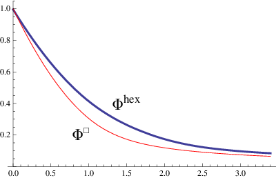
Estimate (1.2) is discussed in Remark 2 of Section 5. The repartition function $\Phi^{\mathrm{hex}}$ can be explicitly computed as

\Phi^{\mathrm{hex}}(\xi)=\frac{4}{\pi^{2}}\ G\left(\frac{2\xi}{\sqrt{3}}\right),

(1.3)

with $G(\xi)$ obtained by adding all terms $\frac{\zeta(2)}{c_{I}}G_{I,Q}^{(*)}$ from formulas (5.22), (6.6), (6.7), (6.8), (6.9), (6.10), (6.11), (7.1), (7.2), (7.5), (7.6), (7.8), (7.11), (7.12), (7.13), (8.1), (8.2), (8.5), (8.6), (8.8), (8.9), (8.10), (8.11), (8.12), (8.13), (8.14), (9.1), (9.2), (9.4), (9.5), (9.6), (9.7), (9.9), (9.10), (9.11), (9.12), (9.13), (9.14), (9.15) and (9.16).

In the case of the square lattice only the term from (5.22) arises, with a different constant and no $\frac{2}{\sqrt{3}}$ scaling for $\xi$ . The limiting distribution $\Phi^{\square}$ also satisfies (1.2).

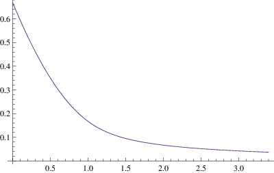
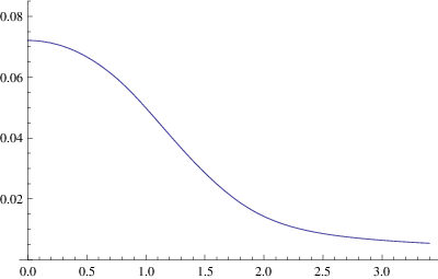
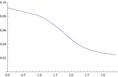
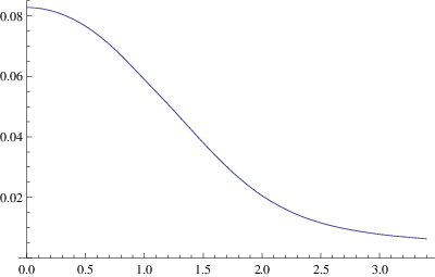
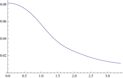
Refer to caption — Figure 2. The limiting repartition functions $\Phi^{\mathrm{hex}}$ and $\Phi^{\square}$

In the case of a lattice it was actually proved in [16] that for every ${\mathbf{x}}\in{\mathbb{R}}^{2}\setminus{\mathbb{Q}}^{2}$ , $\lim_{\varepsilon\rightarrow 0^{+}}\frac{1}{2\pi}\big|\big\{\omega\in[0,2\pi):\varepsilon\tau_{\varepsilon}^{\square}({\mathbf{x}},\omega)>\xi\big\}\big|=\Phi^{\square}(\xi)$ . It would be interesting to know whether a similar result holds true for a generic choice of ${\mathbf{x}}$ in the case of the honeycomb.

The analog problem about the free path length in a regular polygon with $n$ sides ( $n\neq 3,4,6$ ) seems to be out of reach at this time, due to lack of a tractable coding for the linear flow. In the case of the regular octogon the recent results in [20] may prove helpful.

2. Translating the problem to the square lattice with $\hskip-6.0pt\mod{3}$ constraints

For manifest symmetry reasons it suffices to consider ${\mathbf{x}}\in H_{\varepsilon}$ and $\omega\in\big[0,\frac{\pi}{6}\big]$ , or equivalently $t=\tan\omega\in\big[0,\frac{1}{\sqrt{3}}\big]$ . We will simply write $\tau_{\varepsilon}^{\mathrm{hex}}({\mathbf{x}},\omega)=\tau^{\mathrm{hex}}_{\varepsilon}({\mathbf{x}},t)$ . As in [3] consider the lattice ${\mathbb{Z}}^{2}M_{0}$ , $M_{0}=\left(\begin{smallmatrix}1&0\\ 1/2&\sqrt{3}/2\end{smallmatrix}\right)$ , and the linear transformation $T{\mathbf{x}}={\mathbf{x}}M_{0}^{-1}$ on ${\mathbb{R}}^{2}$ :

T(x,y)=\left(x-\frac{y}{\sqrt{3}},\frac{2y}{\sqrt{3}}\right)=(x^{\prime},y^{\prime}).

This maps the vertices $\big(q+\frac{a}{2},\frac{a\sqrt{3}}{2}\big)$ of the grid of equilateral triangles of unit side onto the vertices $(q,a)$ of the square lattice ${\mathbb{Z}}^{2}$ . The vertices of the honeycomb are mapped exactly into ${\mathbb{Z}}^{2}_{(3)}$ , the subset of elements of ${\mathbb{Z}}^{2}$ with $q\nequiv a\pmod{3}$ (see Figure 3). The points of the $x$ -axis are fixed by $T$ . The circular scatterers $S_{q,a,\varepsilon}=(x_{0},y_{0})+\varepsilon(\cos\theta,\sin\theta)$ with $(x_{0},y_{0})=\big(q+\frac{a}{2},\frac{a\sqrt{3}}{2}\big)$ are mapped onto ellipsoidal scatterers $(x_{0}^{\prime},y_{0}^{\prime})+\varepsilon\big(\cos\theta-\frac{\sin\theta}{\sqrt{3}},\frac{2\sin\theta}{\sqrt{3}}\big)$ centered at $(x_{0}^{\prime},y_{0}^{\prime})=(q,a)=T(x_{0},y_{0})$ . The channel of width $w=2\varepsilon$ , bounded by the two lines of slope $t=\tan\omega$ and tangent to the circle $S_{q,a,\varepsilon}$ , is mapped (see Figure 4) onto the channel of width $w^{\prime}=2\varepsilon^{\prime}\cos\omega^{\prime}$ , bounded by the two lines tangent to the ellipse $T(S_{q,a,\varepsilon})$ , of slope $t^{\prime}=\tan\omega^{\prime}=\Psi(t)$ , where

\Psi:\left[0,\frac{1}{\sqrt{3}}\right]\rightarrow[0,1],\quad t^{\prime}=\Psi(t)=\frac{2t}{\sqrt{3}-t},\quad t=\Psi^{-1}(t^{\prime})=\frac{t^{\prime}\sqrt{3}}{t^{\prime}+2}.

The intersection of these two channels and the $x$ -axis is the horizontal segment centered at the origin, of length

\frac{2\varepsilon}{\sin\omega}=\frac{w}{\sin\omega}=\frac{w^{\prime}}{\sin\omega^{\prime}}=\frac{2\varepsilon^{\prime}}{\tan\omega^{\prime}}.

In particular

\varepsilon^{\prime}=\varepsilon^{\prime}(\omega,\varepsilon)=\frac{\varepsilon\tan\omega^{\prime}}{\sin\omega}=\frac{\varepsilon}{\cos(\pi/6+\omega)}.

(2.1)

We can first replace each circular scatterer $S_{q,a,\varepsilon}$ by the segment $\tilde{S}_{q,a,\varepsilon}$ centered at $(x_{0},y_{0})$ , of slope $\frac{\pi}{3}$ and length $\frac{2\varepsilon}{\cos(\pi/6+\omega)}=2\varepsilon^{\prime}$ (see Figures 3 and 4). Indeed, this change will result in altering, for each $\omega$ , the free path length $\tau_{\varepsilon}^{\mathrm{hex}}({\mathbf{x}},t)$ to the free path length $\tilde{\tau}_{\varepsilon}^{\mathrm{hex}}({\mathbf{x}},t)$ corresponding to the later model by a quantity lesser than $4\sqrt{3}\varepsilon^{2}$ , which is insignificant for the final result.

Next we apply $T$ to transport the problem from the honeycomb to the square lattice with congruence $\hskip-6.0pt\pmod{3}$ constraints (or in the opposite direction through $T^{-1}$ ). The unit regular hexagon $H$ centered at the origin is mapped to the hexagon $T(H)$ which contains $(0,0)$ in Figure 4. Actually it will be more convenient to replace $T(H)$ by the fundamental domain $F$ consisting of the union of the square $[0,1)^{2}$ and of its translates $[-1,0)\times[0,1)$ and $[0,1)\times[-1,0)$ . Let $\varepsilon^{\prime}=\varepsilon^{\prime}(\omega,\varepsilon)$ be as in (2.1), $t^{\prime}=\tan\omega^{\prime}$ as above, and consider the vertical segment $V_{\varepsilon^{\prime}}=\{0\}\times[-\varepsilon^{\prime},\varepsilon^{\prime}]$ . Consider

\tilde{q}_{\varepsilon^{\prime}}^{\square}({\mathbf{x}}^{\prime},t^{\prime})=\inf\{n\in{\mathbb{N}}_{0}:{\mathbf{x}}^{\prime}+(n,nt^{\prime})\in{\mathbb{Z}}^{2}_{(3)}+V_{\varepsilon^{\prime}}\},

the horizontal free path length in the square lattice with vertical scatterers of (nonconstant) length $2\varepsilon^{\prime}$ centered at points $(x_{0}^{\prime},y_{0}^{\prime})=(q,a)\in{\mathbb{Z}}^{2}_{(3)}$ . Consider also $q_{\varepsilon_{0}}^{\square}({\mathbf{x}}^{\prime},t^{\prime})$ , the horizontal free path in the square lattice with vertical scatterers of constant length $2\varepsilon_{0}$ centered at points $(x_{0}^{\prime},y_{0}^{\prime})=(q,a)\in{\mathbb{Z}}^{2}_{(3)}$ . Clearly $q^{\square}_{\varepsilon_{+}}({\mathbf{x}}^{\prime},t^{\prime})\leqslant\tilde{q}^{\square}_{\varepsilon^{\prime}}({\mathbf{x}}^{\prime},t^{\prime})\leqslant q^{\square}_{\varepsilon_{-}}({\mathbf{x}}^{\prime},t^{\prime})$ when $t^{\prime}$ belongs to an interval $I^{\prime}$ and $\varepsilon_{-}\leqslant\varepsilon^{\prime}=\varepsilon^{\prime}(t^{\prime})\leqslant\varepsilon^{+}$ , $\forall t^{\prime}\in I^{\prime}$ .

For each angle $\omega^{\prime}$ the transformation $T$ maps $H$ onto $F$ and $T^{-1}$ preserves the structure of channels in the corresponding three-strip partition from [1, 7, 9] (see also the expository paper [13]). Removal of vertical scatterers $V_{q,a,\varepsilon^{\prime}}=T(\tilde{S}_{q,a,\varepsilon})$ with $q\equiv a\pmod{3}$ in the ${\mathbb{Z}}^{2}_{(3)}$ picture results in dividing the corresponding channel of the three-strip partition from the square lattice model into several sub-channels, and in the occurrence of longer trajectories associated with them. This is transported by $T^{-1}$ back to the honeycomb model. The key observation here is that, by the Rule of Sines,

\frac{\tilde{\tau}^{\mathrm{hex}}_{\varepsilon}({\mathbf{x}},t)}{\sin(2\pi/3)}=\frac{\tilde{q}^{\square}_{\varepsilon^{\prime}}(T{\mathbf{x}},t^{\prime})}{\sin(\pi/3-\omega)}=\frac{\tilde{q}^{\square}_{\varepsilon^{\prime}}(T{\mathbf{x}},t^{\prime})}{\cos(\pi/6+\omega)}.

This shows that

\tilde{\tau}^{\mathrm{hex}}_{\varepsilon}({\mathbf{x}},t)>\frac{\xi}{\varepsilon}\quad\Longleftrightarrow\quad\tilde{q}^{\square}_{\varepsilon^{\prime}}(T{\mathbf{x}},t^{\prime})>\frac{2\xi\cos(\pi/6+\omega)}{\varepsilon\sqrt{3}}=\frac{\xi^{\prime}}{\varepsilon^{\prime}},\quad\xi^{\prime}:=\frac{2\xi}{\sqrt{3}},

(2.2)

leading to

\chi_{\big(\frac{\xi}{\varepsilon},\infty\big)}\Big(\tilde{\tau}_{\varepsilon}^{\mathrm{hex}}({\mathbf{x}},t)\Big)=\chi_{\big(\frac{\xi^{\prime}}{\varepsilon^{\prime}},\infty\big)}\Big(\tilde{q}^{\square}_{\varepsilon^{\prime}}(T{\mathbf{x}},t^{\prime})\Big),\quad\forall{\mathbf{x}}\in H,\forall t\in\left[0,\frac{1}{\sqrt{3}}\right].

For each interval $I=[\tan\omega_{0},\tan\omega_{1}]\subseteq\big[0,\frac{1}{\sqrt{3}}\big]$ one has

\begin{split}\varepsilon^{-}_{I}:=\frac{\varepsilon}{\cos(\pi/6+\omega_{0})}\leqslant\varepsilon^{\prime}&=\frac{\varepsilon}{\cos(\pi/6+\omega)}\leqslant\varepsilon^{+}_{I}:=\frac{\varepsilon}{\cos(\pi/6+\omega_{1})},\\ \varepsilon^{\pm}_{I}&=\big(1+O|I|)\big)\varepsilon.\end{split}

Employing now (2.2) and the fact that $\varepsilon\mapsto\tilde{q}_{\varepsilon}^{\square}(T{\mathbf{x}},t^{\prime})$ is non-decreasing, and taking

\xi^{-}_{I}:=\frac{\xi^{\prime}\varepsilon^{-}_{I}}{\varepsilon^{+}_{I}}\leqslant\xi^{\prime}\leqslant\xi^{+}_{I}:=\frac{\xi^{\prime}\varepsilon^{+}_{I}}{\varepsilon^{-}_{I}},\quad\xi^{\pm}_{I}=\big(1+O(|I|)\big)\xi^{\prime},

we infer

\begin{split}\chi_{\big(\frac{\xi^{+}_{I}}{\varepsilon^{+}_{I}},\infty\big)}\Big(q_{\varepsilon^{+}_{I}}^{\square}(T{\mathbf{x}},t^{\prime})\Big)&=\chi_{\big(\frac{\xi^{\prime}}{\varepsilon^{-}_{I}},\infty\big)}\Big(q_{\varepsilon^{+}_{I}}^{\square}(T{\mathbf{x}},t^{\prime})\Big)\leqslant\chi_{\big(\frac{\xi^{\prime}}{\varepsilon^{\prime}},\infty\big)}\Big(q_{\varepsilon^{+}_{I}}^{\square}(T{\mathbf{x}},t^{\prime})\Big)\\ &\leqslant\chi_{\big(\frac{\xi^{\prime}}{\varepsilon^{\prime}},\infty\big)}\Big(\tilde{q}^{\square}_{\varepsilon^{\prime}}(T{\mathbf{x}},t^{\prime})\Big)=\chi_{\big(\frac{\xi}{\varepsilon},\infty\big)}\Big(\tilde{\tau}^{\mathrm{hex}}_{\varepsilon}({\mathbf{x}},t)\Big)\leqslant\chi_{\big(\frac{\xi^{\prime}}{\varepsilon^{\prime}},\infty\big)}\Big(q_{\varepsilon^{-}_{I}}^{\square}(T{\mathbf{x}},t^{\prime})\Big)\\ &\leqslant\chi_{\big(\frac{\xi^{\prime}}{\varepsilon^{+}_{I}},\infty\big)}\Big(q_{\varepsilon^{-}_{I}}^{\square}(T{\mathbf{x}},t^{\prime})\Big)=\chi_{\big(\frac{\xi^{-}_{I}}{\varepsilon^{-}_{I}},\infty\big)}\Big(q_{\varepsilon^{-}_{I}}^{\square}(T{\mathbf{x}},t^{\prime})\Big).\end{split}

Consider

\mathbb{G}_{I,\varepsilon}(\xi):=\int_{\Psi(I)}\frac{dt^{\prime}}{t^{\prime 2}+t^{\prime}+1}\int_{F}d{\mathbf{x}}^{\prime}\,\chi_{\big(\frac{\xi}{\varepsilon},\infty\big)}\Big(q^{\square}_{\varepsilon}({\mathbf{x}}^{\prime},t^{\prime})\Big).

(2.3)

Applying the change of variable $({\mathbf{x}}^{\prime},t^{\prime})=\big(T{\mathbf{x}},\Psi(t)\big)$ and employing (2.3), $d{\mathbf{x}}=\frac{\sqrt{3}}{2}d{\mathbf{x}}^{\prime}$ and $\frac{dt}{t^{2}+1}=\frac{\sqrt{3}}{2}\cdot\frac{dt^{\prime}}{t^{\prime 2}+t^{\prime}+1}$ we infer

\begin{split}\frac{3}{4}\,\mathbb{G}_{I,\varepsilon^{+}_{I}}(\xi^{+}_{I})&\leqslant\frac{3}{4}\int_{\Psi(I)}\frac{dt^{\prime}}{t^{\prime 2}+t^{\prime}+1}\int_{F}d{\mathbf{x}}^{\prime}\,\chi_{\big(\frac{\xi^{+}_{I}}{\varepsilon^{+}_{I}},\infty\big)}\Big(q^{\square}_{\varepsilon^{+}_{I}}({\mathbf{x}}^{\prime},t^{\prime})\Big)\\ &\leqslant\widetilde{\mathbb{P}}_{I,\varepsilon}(\xi):=\iint_{H\times I}\chi_{\big(\frac{\xi}{\varepsilon},\infty\big)}\Big(\tilde{\tau}_{\varepsilon}^{\mathrm{hex}}({\mathbf{x}},\omega)\Big)\,d{\mathbf{x}}d\omega\\ &=\int_{I}\frac{dt}{t^{2}+1}\int_{H}d{\mathbf{x}}\,\chi_{\big(\frac{\xi}{\varepsilon},\infty\big)}\Big(\tilde{\tau}^{\mathrm{hex}}_{\varepsilon}({\mathbf{x}},t)\Big)\\ &\leqslant\frac{3}{4}\int_{\Psi(I)}\frac{dt^{\prime}}{t^{\prime 2}+t^{\prime}+1}\int_{F}d{\mathbf{x}}^{\prime}\,\chi_{\big(\frac{\xi^{-}_{I}}{\varepsilon^{-}_{I}},\infty\big)}\Big(q^{\square}_{\varepsilon^{-}_{I}}({\mathbf{x}}^{\prime},t^{\prime})\Big)=\frac{3}{4}\,\mathbb{G}_{I,\varepsilon^{-}_{I}}(\xi^{-}_{I}).\end{split}

To simplify notation we simply denote $\mathbb{G}_{I,1/(2Q)}$ by $\mathbb{G}_{I,Q}$ throughout. We shall employ the following result, whose proof occupies the remaining part of the paper.

Theorem 2.

Let $c,c^{\prime}>0$ such that $c+c^{\prime}<1$ . For every interval $I\subseteq[0,1]$ of length $|I|\asymp Q^{c}$ , every $\xi\geqslant 0$ and $\delta>0$ , uniformly for $\xi$ in compact subsets $K$ of $[0,\infty)$ ,

\mathbb{G}_{I,Q}(\xi)=\frac{2c_{I}}{\zeta(2)}\,G(\xi)+O_{\delta,K}\big(E_{c,c^{\prime},\delta}(Q)\big),

(2.4)

where $G(\xi)$ is the 40 term sum described below (1.3) and

c_{I}=\int_{I}\frac{dt}{t^{2}+t+1},\quad c_{[0,1]}=\frac{\pi}{3\sqrt{3}},

E_{c,c^{\prime},\delta}(Q)=Q^{\max\big\{2c^{\prime}-\frac{1}{2},-c-c^{\prime}\big\}+\delta}.

(2.5)

Proof.

Proof of Theorem 1. Let $Q^{-}=Q^{-}_{I}:=\Big\lfloor\frac{1}{2\varepsilon_{I}^{-}}\Big\rfloor+1$ and $\frac{\varepsilon_{I}^{-}}{1+2\varepsilon_{I}^{-}}\leqslant\varepsilon^{-}:=\frac{1}{2Q^{-}}\leqslant\varepsilon_{I}^{-}$ . Then $q^{\square}_{\varepsilon_{I}^{-}}({\mathbf{x}}^{\prime},t^{\prime})\leqslant q^{\square}_{\varepsilon^{-}}({\mathbf{x}}^{\prime},t^{\prime})$ , so $\chi_{(\xi_{I}^{-}/\varepsilon_{I}^{-},\infty)}\big(q^{\square}_{\varepsilon_{I}^{-}}({\mathbf{x}}^{\prime},t^{\prime})\big)\leqslant\chi_{(\xi_{I}^{-}/\varepsilon_{I}^{-},\infty)}\big(q^{\square}_{\varepsilon_{-}}({\mathbf{x}}^{\prime},t^{\prime})\big)$ . Similarly, taking $Q^{+}=Q^{+}_{I}:=\Big\lfloor\frac{1}{2\varepsilon_{I}^{+}}\Big\rfloor$ , $\varepsilon_{I}^{+}\leqslant\varepsilon^{+}:=\frac{1}{2Q^{+}}\leqslant\frac{\varepsilon_{I}^{+}}{1-2\varepsilon_{I}^{+}}$ , we have $\chi_{(\xi_{I}^{+}/\varepsilon_{I}^{+},\infty)}\big(q^{\square}_{\varepsilon_{I}^{+}}({\mathbf{x}}^{\prime},t^{\prime})\big)\geqslant\chi_{(\xi_{I}^{+}/\varepsilon_{I}^{+},\infty)}\big(q^{\square}_{\varepsilon^{+}}({\mathbf{x}}^{\prime},t^{\prime})\big)$ . On the other hand $\frac{\varepsilon^{\pm}}{\varepsilon^{\pm}_{I}}=1+O(\varepsilon)$ , hence

\frac{\xi_{I}^{\pm}}{\varepsilon_{I}^{\pm}}=\frac{\xi_{I}^{\pm}}{\varepsilon^{\pm}}\cdot\frac{\varepsilon^{\pm}}{\varepsilon^{\pm}_{I}}=\big(1+O(|I|)\big)\,\frac{\xi^{\prime}}{\varepsilon^{\pm}}.

We now infer

\begin{split}\mathbb{G}_{I,Q^{+}}\Big(\big(1+O(|I|)\big)\xi^{\prime}\Big)&\leqslant\frac{3}{4}\mathbb{G}_{I,\varepsilon_{I}^{+}}(\xi_{I}^{+})\leqslant\widetilde{\mathbb{P}}_{I,\varepsilon}(\xi)\\ &\leqslant\frac{3}{4}\,\mathbb{G}_{I,\varepsilon_{I}^{-}}(\xi_{I}^{-})\leqslant\frac{3}{4}\mathbb{G}_{I,Q^{-}}\Big(\big(1+O(|I|)\big)\xi^{\prime}\Big).\end{split}

(2.6)

Partition now the interval $\big[0,\frac{1}{\sqrt{3}}\big]$ as a union of $N=\big[\varepsilon^{-c}\big]$ intervals $I_{j}=[\tan\omega_{j},\tan\omega_{j+1}]$ of equal length $|I_{j}|=\frac{1}{N}\asymp\varepsilon^{c}$ , with $0<c<1$ to be chosen later. As above, consider $Q_{j}^{\pm}=Q_{I_{j}}^{\pm}$ . The intervals $\Psi(I_{j})$ partition $[0,1]$ and $|\Psi(I_{j})|\asymp\varepsilon^{c}$ . Applying (2.6), Theorem 2 and the property of $G$ of being Lipschitz on the compact $K$ we infer

\begin{split}{\mathbb{P}}_{\varepsilon}^{\mathrm{hex}}(\xi)&=\frac{6}{\pi|H|}\sum_{j=1}^{N}\widetilde{\mathbb{P}}_{I_{j},\varepsilon}(\xi)=\frac{\sqrt{3}}{\pi}\sum_{j=1}^{N}\mathbb{G}_{I_{j},Q_{j}^{\pm}}(\xi)\\ &=\frac{2\sqrt{3}}{\pi\zeta(2)}\sum_{j=1}^{N}c_{I_{j}}G\left(\Big(1+O(|I|)\Big)\frac{2\xi}{\sqrt{3}}\right)+O_{\delta,K}\big(N\varepsilon^{-\max\{2c_{1}-\frac{1}{2},-c-c_{1}\}}\big)\\ &=\frac{2c_{[0,1]}\sqrt{3}}{\pi\zeta(2)}\,G\left(\frac{2\xi}{\sqrt{3}}\right)+O_{\delta,K}\big(\varepsilon^{-c}+\varepsilon^{-\max\{c+2c_{1}-\frac{1}{2},-c_{1}\}-\delta}\big),\end{split}

uniformly for $\xi$ in compacts of $[0,\infty)$ . Taking $c=c_{1}=\frac{1}{8}$ we find

{\mathbb{P}}_{\varepsilon}^{\mathrm{hex}}(\xi)=\frac{4}{\pi^{2}}\,G\left(\frac{2\xi}{\sqrt{3}}\right)+O_{\delta,K}\big(\varepsilon^{\frac{1}{8}-\delta}\big),

as stated in Theorem 1 and in (1.3). ∎

3. Some number theoretical estimates

In this section we review and prove some number theoretical estimates that will be further used to estimate certain sums over integer lattice points with congruence constraints. The principal Dirichlet character $\hskip-3.0pt\pmod{\ell}$ will be denoted by $\chi_{0}$ . The number of divisors of $N$ is denoted by $\sigma_{0}(N)$ .

Lemma 1 (Lemma 2.2 of [2]).

For each function $f\in C^{1}[0,N]$ with total variation $T_{0}^{N}f$ ,

\sum\limits_{\begin{subarray}{c}1\leqslant q\leqslant N\\ (q,\ell)=1\end{subarray}}f(q)=\frac{\varphi(\ell)}{\ell}\int_{0}^{N}f(x)\,dx+O\Big((\|f\|_{\infty}+T_{0}^{N}f)\sigma_{0}(N)\Big).

Lemma 2 (Lemma 2.1 of [3]).

For each function $V\in C^{1}[0,N]$ ,

\sum\limits_{\begin{subarray}{c}1\leqslant q\leqslant N\\ (q,\ell)=1\end{subarray}}\frac{\varphi(q)}{q}V(q)=C(\ell)\int_{0}^{N}V(x)\,dx+O_{\ell}\Big((\|V\|_{\infty}+T_{0}^{N}V)\log N\Big),

where

C(\ell)=\frac{\varphi(\ell)}{\zeta(2)\ell}\prod\limits_{\begin{subarray}{c}p\in{\mathcal{P}}\\ p\mid\ell\end{subarray}}\left(1-\frac{1}{p^{2}}\right)^{-1}=\frac{1}{\zeta(2)}\prod\limits_{\begin{subarray}{c}p\in{\mathcal{P}}\\ p\mid\ell\end{subarray}}\left(1+\frac{1}{p}\right)^{-1}=\frac{\varphi(\ell)}{\ell L(2,\chi_{0})}.

We need a more precise form of Lemma 1, as follows:

Lemma 3.

Suppose that $(r,\ell)=1$ . For each function $V\in C^{1}[0,N]$ ,

\sum\limits_{\begin{subarray}{c}1\leqslant q\leqslant N\\ q\equiv r\hskip-6.0pt\pmod{\ell}\end{subarray}}\frac{\varphi(q)}{q}V(q)=\frac{C(\ell)}{\varphi(\ell)}\int_{0}^{N}V(x)\,dx+O_{\ell}\Big((\|V\|_{\infty}+T_{0}^{N}V)\log N\Big).

In particular

\sum\limits_{\begin{subarray}{c}1\leqslant q\leqslant N\\ q\equiv\pm 1\hskip-6.0pt\pmod{3}\end{subarray}}\frac{\varphi(q)}{q}V(q)\sim\frac{3}{8\zeta(2)}\int_{0}^{N}V(x)\,dx,\quad\sum\limits_{\begin{subarray}{c}1\leqslant q\leqslant N\\ q\equiv 0\hskip-6.0pt\pmod{3}\end{subarray}}\frac{\varphi(q)}{q}V(q)\sim\frac{1}{4\zeta(2)}\int_{0}^{N}V(x)\,dx.

Proof.

When $(k,\ell)=1$ denote by $\bar{k}$ the multiplicative inverse of $k\hskip-3.0pt\pmod{\ell}$ . Let $G=U({\mathbb{Z}}/\ell{\mathbb{Z}})$ denote the multiplicative group of units of ${\mathbb{Z}}/\ell{\mathbb{Z}}$ and $\widehat{G}$ be the group of characters $\chi:G\rightarrow{\mathbb{T}}$ , extended as multiplicative functions on ${\mathbb{N}}$ . Set $V_{d}(x)=V(xd)$ . By Schur’s orthogonality relations for characters, for every $x,s\in{\mathbb{N}}$ with $(s,\ell)=1$ ,

\frac{1}{\varphi(\ell)}\sum_{\chi\in\widehat{G}}\chi(x)\chi(\bar{s})=\frac{1}{\varphi(\ell)}\sum_{\chi\in\widehat{G}}\chi(x)\,\overline{\chi(s)}=\begin{cases}1&\mbox{\rm if $x\equiv s\pmod{\ell},$}\\ 0&\mbox{\rm if $x\nequiv s\pmod{\ell}.$}\end{cases}

(3.1)

Taking $s=r$ and summing over $x=q\leqslant N$ , we infer by Möbius summation, with $q=md$ ,

\begin{split}\sum\limits_{\begin{subarray}{c}q\leqslant N\\ q\equiv r\hskip-6.0pt\pmod{\ell}\end{subarray}}\frac{\varphi(q)}{q}V(q)&=\frac{1}{\varphi(\ell)}\sum_{q\leqslant N}\frac{\varphi(q)}{q}V(q)\sum_{\chi\in\widehat{G}}\chi(q)\chi(\bar{r})\\ &=\frac{1}{\varphi(\ell)}\sum_{q\leqslant N}\sum_{d\mid q}\frac{\mu(d)}{d}V(q)\sum_{\chi\in\widehat{G}}\chi(q)\chi(\bar{r})\\ &=\frac{1}{\varphi(\ell)}\sum_{d\leqslant N}\sum_{m=1}^{\lfloor N/d\rfloor}\sum_{\chi\in\widehat{G}}\frac{\mu(d)}{d}V_{d}(m)\chi(md)\chi(\bar{r})\\ &=\frac{1}{\varphi(\ell)}\sum_{\chi\in\widehat{G}}\chi(\bar{r})\sum_{d\leqslant N}\frac{\mu(d)\chi(d)}{d}\sum_{m=1}^{\lfloor N/d\rfloor}V_{d}(m)\chi(m).\end{split}

(3.2)

We split the inner sum above according to whether $\chi=\chi_{0}$ or $\chi\neq\chi_{0}$ . Employing Lemma 1 for the function $V_{d}$ we find that the contribution of the former is

\begin{split}\frac{1}{\varphi(\ell)}\sum_{d\leqslant N}\frac{\mu(d)\chi_{0}(d)}{d}&\left(\frac{\varphi(\ell)}{\ell}\int_{0}^{\lfloor N/d\rfloor}V_{d}+O\Big((\|V_{d}\|_{\infty}+T_{0}^{N/d}V_{d})\log N\Big)\right)\\ &=\frac{1}{\ell}\left(\ \sum_{d\leqslant N}\frac{\mu(d)\chi_{0}(d)}{d^{2}}\right)\int_{0}^{N}V+O_{\ell}\Big((\|V\|_{\infty}+T_{0}^{N}V)\log N\Big)\\ &=\left(\frac{1}{\ell L(2,\chi_{0})}+O_{\ell}\Big(\frac{1}{N}\Big)\right)\int_{0}^{N}V+O_{\ell}\Big((\|V\|_{\infty}+T_{0}^{N}V)\log N\Big)\\ &=\frac{C(\ell)}{\varphi(\ell)}\int_{0}^{N}V+O_{\ell}\Big((\|V\|_{\infty}+T_{0}^{N}V)\log N\Big).\end{split}

When $\chi\neq\chi_{0}$ we find by partial summation and Pólya-Vinogradov (or a weaker inequality) that the innermost sum in (3.2) is $\ll_{\ell}T_{0}^{N}V+\|V\|_{\infty}$ , so the total contribution of non-principal characters in (3.2) is $\ll_{\ell}\|V\|_{\infty}\log N$ . The proof is complete. ∎

Lemma 4 (Proposition A4 of [6]).

Assume that $q\geqslant 1$ and $h$ are integers, ${\mathcal{I}}$ and ${\mathcal{J}}$ are intervals of length less than $q$ , and $f\in C^{1}({\mathcal{I}}\times{\mathcal{J}})$ . For any integer $T>1$ and any $\delta>0$

\sum\limits_{\begin{subarray}{c}a\in{\mathcal{I}},b\in{\mathcal{J}}\\ (a,q)=1\\ ab\equiv h\hskip-5.0pt\pmod{q}\end{subarray}}f(a,b)=\frac{\varphi(q)}{q^{2}}\iint_{{\mathcal{I}}\times{\mathcal{J}}}f(x,y)\,dx\,dy+\mathcal{E},

with

\mathcal{E}\ll_{\delta}T^{2}\|f\|_{\infty}q^{\frac{1}{2}+\delta}(h,q)^{\frac{1}{2}}+T\|\nabla f\|_{\infty}q^{\frac{3}{2}+\delta}(h,q)^{\frac{1}{2}}+\frac{\|\nabla f\|_{\infty}|{\mathcal{I}}|\,|{\mathcal{J}}|}{T},

where $\|f\|_{\infty}$ and $\|\nabla f\|_{\infty}$ denote the sup-norm of $f$ and respectively $\big|\frac{\partial f}{\partial x}\big|+\big|\frac{\partial f}{\partial y}\big|$ on ${\mathcal{I}}\times{\mathcal{J}}$ .

For $q$ , $\ell$ positive integers denote

A(q,\ell)=\begin{cases}1&\mbox{\rm if $(q,\ell)=1,$}\\ \prod\limits_{\begin{subarray}{c}p\in{\mathcal{P}}\\ p\mid(q,\ell)\end{subarray}}\left(1-\frac{1}{p}\right)^{-1}&\mbox{\rm if $(q,\ell)>1.$}\end{cases}

Lemma 5.

Suppose that $(r,\ell)=1$ . For any interval ${\mathcal{I}}$ , uniformly in $|{\mathcal{I}}|$ ,

\sum\limits_{\begin{subarray}{c}x\in{\mathcal{I}},\,(x,q)=1\\ x\equiv r\hskip-6.0pt\pmod{\ell}\end{subarray}}1=\frac{A(q,\ell)}{\ell}\cdot\frac{\varphi(q)}{q}\,|{\mathcal{I}}|+O\left(\sigma_{0}(q)\right).

Proof.

Without loss of generality assume ${\mathcal{I}}=[1,N]$ . As in the proof of Lemma 3 take $s=r$ and sum in (3.1) over $x\in{\mathcal{I}}$ with $(x,q)=1$ . By Möbius inversion with $x=md$ we infer

\begin{split}\sum\limits_{\begin{subarray}{c}x\in{\mathcal{I}},\,(x,q)=1\\ x\equiv r\hskip-6.0pt\pmod{\ell}\end{subarray}}1&=\frac{1}{\varphi(\ell)}\sum\limits_{\begin{subarray}{c}x\in{\mathcal{I}}\\ (x,q)=1\end{subarray}}\sum_{\chi\in\widehat{G}}\chi(x)\chi(\bar{r})=\frac{1}{\varphi(\ell)}\sum_{\chi\in\widehat{G}}\sum_{x\in{\mathcal{I}}}\chi(x)\chi(\bar{r})\sum\limits_{\begin{subarray}{c}d\mid q\\ d\mid x\end{subarray}}\mu(d)\\ &=\frac{1}{\varphi(\ell)}\sum_{d\mid q}\mu(d)\sum\limits_{\begin{subarray}{c}x\in{\mathcal{I}}\\ d\mid x\end{subarray}}\sum_{\chi\in\widehat{G}}\chi(x)\chi(\bar{r})=\frac{1}{\varphi(\ell)}\sum_{d\mid q}\mu(d)\sum_{m=1}^{\lfloor N/d\rfloor}\sum_{\chi\in\widehat{G}}\chi(md)\chi(\bar{r}).\end{split}

(3.3)

The contribution of $\chi=\chi_{0}$ to (3.3) is

\begin{split}\frac{1}{\varphi(\ell)}\sum_{d\mid q}\mu(d)\chi_{0}(d)\sum\limits_{\begin{subarray}{c}1\leqslant m\leqslant\lfloor N/d\rfloor\\ (m,\ell)=1\end{subarray}}1&=\frac{1}{\varphi(\ell)}\sum_{d\mid q}\mu(d)\chi_{0}(d)\left(\frac{\varphi(\ell)}{\ell}\bigg(\frac{N}{d}+O(1)\bigg)\right)\\ &=\frac{|{\mathcal{I}}|}{\ell}\sum_{d\mid q}\frac{\mu(d)\chi_{0}(d)}{d}+O\left(\sigma_{0}(q)\right).\end{split}

(3.4)

In the contribution of non-principal characters to (3.3),

\frac{1}{\varphi(\ell)}\sum_{d\mid q}\mu(d)\sum\limits_{\begin{subarray}{c}\chi\in\widehat{G}\\ \chi\neq\chi_{0}\end{subarray}}\chi(d)\chi(\bar{r})\sum_{m=1}^{\lfloor N/d\rfloor}\chi(m),

(3.5)

the innermost sum is $\ll_{\ell}1$ (by Pólya-Vinogradov or a weaker inequality), showing that the quantity in (3.5) is $\ll_{\ell}\sigma_{0}(q)$ . The statement follows now because the sum in (3.4) is equal to $\sum_{d\mid q}\frac{\mu(d)}{d}=\frac{\varphi(q)}{q}$ when $(q,\ell)=1$ , while when $(q,\ell)>1$ , writing $q=p_{1}^{\alpha_{1}}\cdots p_{r}^{\alpha_{r}}\tilde{q}$ with $p_{1},\ldots,p_{r}$ prime divisors of $\ell$ and $(\tilde{q},\ell)=1$ , this sum is equal to

\sum_{d\mid\tilde{q}}\frac{\mu(d)}{d}=\frac{\varphi(\tilde{q})}{\tilde{q}}=\frac{\varphi(q)}{q}\prod\limits_{i=1}^{r}\left(1-\frac{1}{p_{i}}\right)^{-1}=A(q,\ell)\,\frac{\varphi(q)}{q},

as desired. ∎

We also need a slight extension of Lemma 4. Suppose that $(r,\ell)=1$ and denote by $\bar{x}$ the multiplicative inverse of $x\pmod{\ell q}$ when $(x,\ell q)=1$ . The Kloosterman type sums

\begin{split}K(m,n;\ell q)&:=\sum\limits_{\begin{subarray}{c}x\hskip-6.0pt\pmod{\ell q}\\ (x,\ell q)=1\end{subarray}}e\left(\frac{mx+n\bar{x}}{\ell q}\right),\quad\widetilde{K}_{r}(m,n;\ell q):=\sum\limits_{\begin{subarray}{c}x\hskip-6.0pt\pmod{\ell q}\\ (x,q)=1,\,x\equiv r\hskip-6.0pt\pmod{\ell}\end{subarray}}e\left(\frac{mx+n\bar{x}}{\ell q}\right),\\ K_{{\mathcal{I}},r}(m,n;\ell q)&:=\sum\limits_{\begin{subarray}{c}x\in{\mathcal{I}},\,(x,q)=1\\ x\equiv r\hskip-6.0pt\pmod{\ell q}\end{subarray}}e\left(\frac{mx+n\bar{x}}{\ell q}\right),\end{split}

will be used to estimate

\widetilde{N}_{q,\ell,r,h}({\mathcal{I}}_{1},{\mathcal{I}}_{2}):=\#\big\{(x,y)\in{\mathcal{I}}_{1}\times{\mathcal{I}}_{2}:(x,q)=1,x\equiv r\hskip-6.0pt\pmod{\ell},xy\equiv h\hskip-6.0pt\pmod{\ell q}\big\}

Lemma 6.

When $(r,\ell)=1$ , for any interval ${\mathcal{I}}$ of length less than $q$ ,

|K_{{\mathcal{I}},r}(0,n;\ell q)|\ll_{\ell,\delta}(n,q)^{\frac{1}{2}}q^{\frac{1}{2}+\delta}.

Proof.

We write

\begin{split}K_{{\mathcal{I}},r}(0,n;\ell q)&=\sum\limits_{\begin{subarray}{c}x\in{\mathcal{I}},\,(x,q)=1\\ x\equiv r\hskip-6.0pt\pmod{\ell}\end{subarray}}e\left(\frac{n\bar{x}}{\ell q}\right)=\sum\limits_{\begin{subarray}{c}x\hskip-6.0pt\pmod{\ell q}\\ (x,q)=1,\,x\equiv r\hskip-6.0pt\pmod{\ell}\end{subarray}}e\left(\frac{n\bar{x}}{\ell q}\right)\sum_{y\in{\mathcal{I}}}\frac{1}{\ell q}\sum_{k\hskip-6.0pt\pmod{\ell q}}e\left(\frac{k(y-x)}{\ell q}\right)\\ &=\frac{1}{\ell q}\sum_{k\hskip-6.0pt\pmod{\ell q}}\widetilde{K}_{r}(-k,n;\ell q)\sum_{y\in{\mathcal{I}}}e\left(\frac{ky}{\ell q}\right),\end{split}

and

\begin{split}|\widetilde{K}_{r}(m,n;\ell q)|&=\Bigg|\sum\limits_{\begin{subarray}{c}x\hskip-6.0pt\pmod{\ell q}\\ (x,\ell q)=1\end{subarray}}e\left(\frac{mx+n\bar{x}}{\ell q}\right)\frac{1}{\ell}\sum_{j\hskip-6.0pt\pmod{\ell}}e\left(\frac{j(x-r)}{\ell}\right)\Bigg|\\ &=\frac{1}{\ell}\Bigg|\sum_{j\hskip-6.0pt\pmod{\ell}}e\left(-\frac{jr}{\ell}\right)K(m+jq,n;\ell q)\Bigg|\leqslant\max_{j}\left|K(m+jq,n;\ell q)\right|.\end{split}

Employing¹¹ 1 Here $\|x\|=\operatorname{dist}(x,{\mathbb{Z}})$ , $x\in{\mathbb{R}}$ , and $c_{q}(n)=K(n,0;q)=K(0,n;q)$ is the Ramanujan sum.

\Bigg|\sum_{y\in{\mathcal{I}}}e\left(\frac{ky}{\ell q}\right)\Bigg|\leqslant\min\Bigg\{|{\mathcal{I}}|+1,\frac{1}{2\big\|\frac{k}{\ell q}\big\|}\Bigg\},

(3.6)

|K(0,n;\ell q)|=|c_{\ell q}(n)|\leqslant(n,\ell q)\leqslant(n,q)\ell\ll_{\ell}(n,q)^{\frac{1}{2}}q^{\frac{1}{2}},

and the Weil estimate

|K(m+jq,n;\ell q)|\leqslant\sigma_{0}(\ell q)(m+jq,n,\ell q)^{\frac{1}{2}}(\ell q)^{\frac{1}{2}}\ll_{\ell,\delta}(n,q)^{\frac{1}{2}}q^{\frac{1+\delta}{2}},

we infer

\begin{split}|K_{{\mathcal{I}},r}(0,n;\ell q)|&\leqslant\frac{|{\mathcal{I}}|+1}{\ell q}\,|\widetilde{K}_{r}(0,n;\ell q)|+\frac{1}{\ell q}\sum\limits_{\begin{subarray}{c}k\hskip-6.0pt\pmod{\ell q}\\ k\neq 0\end{subarray}}\frac{|\widetilde{K}_{r}(-k,n;\ell q)|}{\big\|\frac{k}{\ell q}\big\|}\\ &\ll_{\ell,\delta}(n,q)^{\frac{1}{2}}q^{\frac{1+\delta}{2}}+\frac{1}{2\ell q}\cdot(n,q)^{\frac{1}{2}}q^{\frac{1+\delta}{2}}\ell q\log(\ell q)\ll_{\ell}(n,q)^{\frac{1}{2}}q^{\frac{1}{2}+\delta},\end{split}

as desired. ∎

Lemma 7.

Suppose that $(r,\ell)=1$ . For any intervals ${\mathcal{I}}_{1}$ and ${\mathcal{I}}_{2}$ of length less than $q$ , any integer $h$ and any $\delta>0$ ,

\widetilde{N}_{q,\ell,r,h}({\mathcal{I}}_{1},{\mathcal{I}}_{2})=\frac{A(q,\ell)}{\ell^{2}}\cdot\frac{\varphi(q)}{q^{2}}\,|{\mathcal{I}}_{1}|\,|{\mathcal{I}}_{2}|+O_{\ell,\delta}\Big((h,q)^{\frac{1}{2}}q^{\frac{1}{2}+\delta}\Big).

Proof.

We write

\widetilde{N}_{q,\ell,r,h}({\mathcal{I}}_{1},{\mathcal{I}}_{2})=\sum\limits_{\begin{subarray}{c}x\in{\mathcal{I}}_{1},\,y\in{\mathcal{I}}_{2}\\ (x,q)=1,\,x\equiv r\hskip-6.0pt\pmod{\ell}\end{subarray}}\frac{1}{\ell q}\sum_{k\hskip-6.0pt\pmod{\ell q}}e\left(\frac{k(y-h\bar{x})}{\ell q}\right)=M+E,

where $\bar{x}$ denotes the multiplicative inverse of $x\pmod{\ell q}$ and

\begin{split}E=&\frac{1}{\ell q}\sum\limits_{\begin{subarray}{c}k\hskip-6.0pt\pmod{\ell q}\\ k\neq 0\end{subarray}}\left(\,\sum_{y\in{\mathcal{I}}_{2}}e\left(\frac{ky}{\ell q}\right)\right)K_{{\mathcal{I}}_{1},r}(0,-hk;\ell q),\\ M=&\frac{1}{\ell q}\sum\limits_{\begin{subarray}{c}x\in{\mathcal{I}}_{1},\,y\in{\mathcal{I}}_{2}\\ (x,q)=1,\,x\equiv r\hskip-6.0pt\pmod{\ell}\end{subarray}}1=\frac{1}{\ell q}\left(\frac{A(q,\ell)}{\ell}\cdot\frac{\varphi(q)}{q}\,|{\mathcal{I}}_{1}|+O\left(\sigma_{0}(q)\right)\right)\Big(|{\mathcal{I}}_{2}|+O(1)\Big)\\ =&\frac{A(q,\ell)}{\ell^{2}}\cdot\frac{\varphi(q)}{q^{2}}\,|{\mathcal{I}}_{1}|\,|{\mathcal{I}}_{2}|+O_{\ell}\left(\sigma_{0}(q)\right).\end{split}

(3.7)

From (3.6), Lemma 6 and $(hk,\ell q)\leqslant(h,q)(k,q)\ell$ , we infer as in the proof of [6, Proposition A.3]

\begin{split}|E|&\ll_{\ell,\delta}q^{-\frac{1}{2}+\frac{\delta}{2}}\sum\limits_{\begin{subarray}{c}k\hskip-6.0pt\pmod{\ell q}\\ k\neq 0\end{subarray}}\frac{(hk,\ell q)^{1/2}}{\big\|\frac{k}{\ell q}\big\|}\ll_{\ell,\delta}q^{-\frac{1}{2}+\frac{\delta}{2}}(h,q)^{\frac{1}{2}}\sum\limits_{\begin{subarray}{c}k\hskip-6.0pt\pmod{\ell q}\\ k\neq 0\end{subarray}}\frac{(k,q)^{1/2}}{\big\|\frac{k}{\ell q}\big\|}\\ &\ll q^{\frac{1+\delta}{2}}(h,q)^{\frac{1}{2}}\sum_{1\leqslant k\leqslant(q-1)/2}\frac{(k,q)^{1/2}}{k}\ll_{\delta}(h,q)^{\frac{1}{2}}q^{\frac{1}{2}+\delta}.\end{split}

(3.8)

The statement follows now from (3.7) and (3.8). ∎

Lemma 8.

Suppose that $(r,\ell)=1$ . Let ${\mathcal{I}}_{1}$ , ${\mathcal{I}}_{1}$ be intervals of length less than $q$ , $f\in C^{1}({\mathcal{I}}_{1}\times{\mathcal{I}}_{2})$ , and $h\in{\mathbb{Z}}$ . For any integer $T>1$ and any $\delta>0$ ,

\sum\limits_{\begin{subarray}{c}x\in{\mathcal{I}}_{1},y\in{\mathcal{I}}_{2}\\ (x,q)=1,\,x\equiv r\hskip-6.0pt\pmod{\ell}\\ xy\equiv h\hskip-5.0pt\pmod{\ell q}\end{subarray}}f(x,y)=\frac{A(q,\ell)}{\ell^{2}}\cdot\frac{\varphi(q)}{q^{2}}\iint_{{\mathcal{I}}_{1}\times{\mathcal{I}}_{2}}f(u,v)\,du\,dv+\mathcal{E},

with

\mathcal{E}\ll_{\ell,\delta}T^{2}\|f\|_{\infty}q^{\frac{1}{2}+\delta}(h,q)^{\frac{1}{2}}+T\|\nabla f\|_{\infty}q^{\frac{3}{2}+\delta}(h,q)^{\frac{1}{2}}+\frac{\|\nabla f\|_{\infty}|{\mathcal{I}}_{1}||{\mathcal{I}}_{2}|}{T}.

Proof.

This plainly follows from Lemma 7 as in the proof of [4, Lemma 2.2]. ∎

Only the case $\ell=3$ and $x\equiv r\nequiv 0\hskip-3.0pt\pmod{3}$ is needed here, with main term given by

\sum\limits_{\begin{subarray}{c}x\in{\mathcal{I}}_{1},\,y\in{\mathcal{I}}_{2}\\ (x,q)=1,\,x\equiv r\hskip-6.0pt\pmod{3}\\ xy\equiv h\hskip-6.0pt\pmod{3q}\end{subarray}}f(x,y)\sim\frac{\varphi(q)}{q^{2}}\left(\iint_{{\mathcal{I}}_{1}\times{\mathcal{I}}_{2}}f(x,y)\,dx\,dy\right)\cdot\begin{cases}\frac{1}{9}&\mbox{\rm if $3\nmid q,$}\\ \frac{1}{6}&\mbox{\rm if $3\mid q.$}\end{cases}

4. Coding the linear flow in ${\mathbb{Z}}^{2}_{(3)}$ and the three-strip partition

To keep notation short denote

x\vee y=\max\{x,y\},\quad x\wedge y=\min\{x,y\},\quad x_{+}=\max\{x,0\}.

Consider $c,c^{\prime},\delta,\xi$ and $I$ as in the statement of Theorem 2 and $E_{c,c^{\prime},\delta}(Q)$ as in (2.5). For $(A_{Q})$ , $(B_{Q})$ sequences of real numbers we write $A_{Q}\approxeq B_{Q}$ when $A_{Q}=B_{Q}+O_{\delta,\xi}\big(E_{c,c^{\prime},\delta}(Q)\big)$ , uniformly for $\xi$ in compact subsets of $[0,\infty)$ . Our primary aim is to estimate the quantity $\mathbb{G}_{I,Q}(\xi)$ from Theorem 2, associated with lattice points from ${\mathbb{Z}}^{2}_{(3)}$ with corresponding vertical scatterers of width $2\varepsilon=\frac{1}{Q}$ , as $Q\rightarrow\infty$ .

It is useful to recall first the approach and notation from [7]. ${\mathcal{F}}(Q)$ denotes the set of Farey fractions of order $Q$ , consisting of rational numbers $\gamma=\frac{a}{q}$ , $0<a\leqslant q\leqslant Q$ , with $(a,q)=1$ . The interval $I$ will be first partitioned into intervals $I_{\gamma}=(\gamma,\gamma^{\prime})$ with $\gamma,\gamma^{\prime}$ consecutive in ${\mathcal{F}}_{I}(Q):={\mathcal{F}}(Q)\cap I$ . Each interval $I_{\gamma}$ is further partitioned into subintervals $I_{\gamma,k}$ , $k\in{\mathbb{Z}}$ , defined as

I_{\gamma,k}=(t_{k},t_{k-1}],\quad I_{\gamma,0}=(t_{0},u_{0}],\quad I_{\gamma,-k}=(u_{k-1},u_{k}],\quad k\in{\mathbb{N}},

where

t_{k}=\frac{a_{k}-2\varepsilon}{q_{k}},\quad u_{k}=\frac{a^{\prime}_{k}+2\varepsilon}{q_{k}^{\prime}},\quad k\in{\mathbb{N}}_{0},

and

q_{k}=q^{\prime}+kq,\quad a_{k}=a^{\prime}+ka,\quad q_{k}^{\prime}=q+kq^{\prime},\quad a_{k}^{\prime}=a+ka^{\prime},\quad k\in{\mathbb{Z}},

satisfy the fundamental relations

\begin{cases}a_{k-1}q_{k}-a_{k}q_{k-1}=1=a_{k-1}q-aq_{k-1},\\ a_{k}^{\prime}q_{k-1}^{\prime}-a_{k-1}^{\prime}q_{k}^{\prime}=1=a^{\prime}q^{\prime}_{k-1}-a^{\prime}_{k-1}q^{\prime},\quad k\in{\mathbb{Z}},\\ 2\varepsilon q_{k}\wedge 2\varepsilon q_{k}^{\prime}\geqslant 2\varepsilon(q+q^{\prime})>1,\quad k\geqslant 1.\end{cases}

Consider also

t:=\tan\omega\quad\mbox{\rm and}\quad\gamma_{k}=\frac{a_{k}}{q_{k}},\quad k\in{\mathbb{N}}.

As it will be seen shortly, the coding of the linear flow is considerably more involved than in the case of the square lattice. As a result our attempt of providing asymptotic results for the repartition of the free path length will require additional partitioning for each of the interval $I_{\gamma,k}$ . For symmetry reasons²² 2 Which are not geometrically obvious but become apparent after translating $\mathbb{G}_{I,Q}(\xi)$ into sums involving (sub)intervals (of) $I_{\gamma,k}$ and Farey fractions from ${\mathcal{F}}_{I}(Q)$ . the mediant intervals $(\gamma,\gamma_{1}]$ and $(\gamma_{1},\gamma^{\prime}]$ will contribute by the same amount to the main term, so we shall only consider $t\in(\gamma,\gamma_{1}]$ and redefine

I_{\gamma,0}:=(t_{0},t_{-1}],\qquad t_{-1}:=\gamma_{1}=\frac{a^{\prime}+a}{q^{\prime}+q}.

This explains the appearance of the factor $2$ in formula (2.4).

As in [7, Section 3] we shall consider³³ 3 Here we use $t=\tan\omega$ as variable and use $\frac{dt}{t^{2}+t+1}$ instead of $d\omega$ ., when $t=\tan\omega\in I_{\gamma,k}$ , $k\in{\mathbb{N}}_{0}$ ,

\begin{split}&w_{\mathcal{A}_{0}}(t)=a+2\varepsilon-qt=q(u_{0}-t),\qquad w_{\mathcal{C}_{k}}(t)=a_{k-1}-2\varepsilon-q_{k-1}t=q_{k-1}(t_{k-1}-t),\\ &w_{\mathcal{B}_{k}}(t)=q_{k}t-a_{k}+2\varepsilon=q_{k}(t-t_{k})\in[0,2\varepsilon],\end{split}

representing the widths of the bottom, center, and respectively top channels $\mathcal{A}_{0}$ , $\mathcal{C}_{k}$ , $\mathcal{B}_{k}$ , of the three-strip partition of $[0,1)^{2}$ (see Figures 5 and 6). Clearly

\begin{cases}2\varepsilon=w_{\mathcal{A}_{0}}(t)+w_{\mathcal{B}_{k}}(t)+w_{\mathcal{C}_{k}}(t),\\ 1=qw_{\mathcal{A}_{0}}(t)+q_{k+1}w_{\mathcal{C}_{k}}(t)+q_{k}w_{\mathcal{B}_{k}}(t),\end{cases}\qquad\forall t\in I_{\gamma,k}.

Recall [7, 9] that in the case of the square lattice the three weights corresponding to $\omega$ are given by

\begin{split}&W_{\mathcal{A}_{0}}(t)=(q-\xi Q)_{+}w_{\mathcal{A}_{0}}(t),\quad W_{\mathcal{B}_{k}}(t)=(q_{k}-\xi Q)_{+}w_{\mathcal{B}_{k}}(t),\\ &W_{\mathcal{C}_{k}}(t)=(q_{k+1}-\xi Q)_{+}w_{\mathcal{C}_{k}}(t).\end{split}

(4.1)

They reflect the area of the parallelogram of height given respectively by $w_{\mathcal{A}_{0}}$ , $w_{\mathcal{C}_{k}}$ or $w_{\mathcal{B}_{k}}$ , and length given by the distance from $\xi Q$ to the bottom of the corresponding sub-channel (if $\xi Q$ is lesser than the total length of the sub-channel).

Figure 5. The three-strip partition of

{\mathbb{R}}^{2}/{\mathbb{Z}}^{2}

when

t\in I_{\gamma,k}

Figure 6. The tiling

{\mathfrak{S}}_{\omega}

of the plane (shaded region represents

{\mathbb{R}}^{2}/{\mathbb{Z}}^{2}

)

The range for $q_{k}=q^{\prime}+kq$ , respectively $q_{k}^{\prime}$ , will be

q_{k}\in{\mathcal{I}}_{q,k}:=\big(Q+(k-1)q,Q+kq\big],\quad\mbox{\rm respectively}\quad q^{\prime}_{k}\in{\mathcal{I}}_{q^{\prime},k}.

Figure 7. The channels

\mathcal{C}_{0}

,

\mathcal{C}_{\leftarrow}

and

\mathcal{C}_{\downarrow}

Denote by $r,r_{k},r^{\prime},r_{k}^{\prime}\in{\mathbb{Z}}/3{\mathbb{Z}}$ the remainders $\hskip-3.0pt\pmod{3}$ of $q-a$ , $q_{k}-a_{k}$ , $q^{\prime}-a^{\prime}$ , $q_{k}^{\prime}-a_{k}^{\prime}$ respectively. The equality $a^{\prime}q-aq^{\prime}=1$ shows that at most one element of the triple $(r,r_{k},r_{k+1})\in({\mathbb{Z}}/3{\mathbb{Z}})^{3}$ can be equal to zero. Similarly, at most one element of the triple $(r^{\prime},r_{k}^{\prime},r_{k+1}^{\prime})$ can be zero.

To ascertain the contribution of the slope $t=\tan\omega\in I_{\gamma,k}$ to $\mathbb{G}_{I,Q}(\xi)$ , we should look at the tiling ${\mathfrak{S}}_{\omega}$ defined by the three-strip partition of ${\mathbb{R}}^{2}$ (shown in Figure 6), but also at ${\mathfrak{S}}_{\omega}^{\leftarrow}$ , its left-horizontal translate by $(1,0)$ , and at ${\mathfrak{S}}_{\omega}^{\downarrow}$ , its down-vertical translate by $(0,1)$ . Since the slits $(m,n)\in{\mathbb{Z}}^{2}$ with $m\equiv n\pmod{3}$ are being removed, sinks are going to arise in the channels. This phenomenon will lead to frequent occurrence of trajectories much longer then in the case of the square lattice. A careful analysis of the bottom of the channels $\mathcal{A}_{0}$ , $\mathcal{C}_{k}$ and $\mathcal{B}_{k}$ is required when the corresponding slit where trajectory ends in the case of the square lattice has been removed. Besides, there is a manifest difference between the three situations where the channel originates at $O=(0,0)$ (this will be referred to as $\mathcal{C}_{O}$ contribution), at $(-1,0)$ ( $\mathcal{C}_{\leftarrow}$ contribution), or at $(-1,0)$ ( $\mathcal{C}_{\downarrow}$ contribution), resulting from the different congruence conditions $\hskip-3.0pt\pmod{3}$ satisfied by the centers of removed slits. This is shown in Figure 6 where the small circles centered at lattice points $(m,n)$ with $m\nequiv n\pmod{3}$ represent the vertical slits of width $2\varepsilon=\frac{1}{Q}$ . We were not able to spot any symmetry that would reduce the analysis to only one of these three types of channels. The contributions to $\Phi^{\mathrm{hex}}$ of the five types of situations that we analyze seem to be quite different (see Figure 19).

To attain a better visualization of the structure of channels we shall represent the slope $\tan\omega$ horizontally. The possible situations are shown in Figure 8, where dotted lines indicate that the corresponding slit has been removed from ${\mathfrak{S}}_{\omega}$ in the case of $\mathcal{C}_{O}$ , from ${\mathfrak{S}}_{\omega}^{\leftarrow}$ in the case of $\mathcal{C}_{\leftarrow}$ and respectively from ${\mathfrak{S}}_{\omega}^{\downarrow}$ in the case of $\mathcal{C}_{\downarrow}$ .

Figure 8. The removed slits for

\mathcal{C}_{O}

,

\mathcal{C}_{\leftarrow}

and

\mathcal{C}_{\downarrow}

To clarify the terminology, by “slit $q_{k}$ ” etc. we will mean the slit which is centered at some lattice point $(q_{k},m)$ and which intersects the channel that is analyzed (there is at most one such point for given $q_{k}$ ).

5. The contribution of channels whose slits are not removed

This resembles the situation of the square lattice and will be discussed in this section. The more intricate situation of the channels where bottom slits are removed will be analyzed in Sections 6-9. When the “first” slit (i.e. the one corresponding to $q$ for $\mathcal{A}_{0}$ , $q_{k+1}$ for $\mathcal{C}_{k}$ , respectively $q_{k}$ for $\mathcal{B}_{k}$ ) is not removed, the table from Figure 8 shows that the corresponding weight is described in the table from Figure 9.

Figure 9. The contribution of channels whose slits are not removed

The weights $W_{\mathcal{A}_{0}}$ , $W_{\mathcal{B}_{k}}$ and $W_{\mathcal{C}_{k}}$ are given by (4.1) as in the case of the square lattice. The cumulative contribution is

\mathbb{G}^{(0)}_{I,Q}(\xi)=\sum_{(\alpha,\beta)\in({\mathbb{Z}}/3{\mathbb{Z}})^{2}\setminus\{(0,0)\}}\mathbb{G}^{(0)}_{I,Q,\alpha,\beta}(\xi),

with $\mathbb{G}^{(0)}_{I,Q,\alpha,\beta}(\xi)$ given by

\sum_{k=0}^{\infty}\hskip-6.0pt\sum\limits_{\begin{subarray}{c}\gamma\in{\mathcal{F}}_{I}(Q)\\ q-a\equiv\alpha\hskip-6.0pt\pmod{3}\\ q_{k}-a_{k}\equiv\beta\hskip-6.0pt\pmod{3}\end{subarray}}\hskip-10.0pt\int_{t_{k}}^{t_{k-1}}\frac{2\big((q-\xi Q)_{+}w_{\mathcal{A}_{0}}(t)+(q_{k+1}-\xi Q)_{+}w_{\mathcal{C}_{k}}(t)+(q_{k}-\xi Q)_{+}w_{\mathcal{B}_{k}}(t)\big)\,dt}{t^{2}+t+1}.

(5.1)

Remark 1..

Putting $x=q-a$ , $y=q_{k}$ , and employing $q_{k}-a_{k}=q_{k}-\frac{1+aq_{k}}{q}=\frac{xy-1}{q}$ , we see that the summation conditions in (5.1) are equivalent to $(x,q)=1$ , $x\equiv\alpha\pmod{3}$ , and $xy\equiv\beta q+1\pmod{3q}$ . Note that $(\beta q+1,q)=1$ and sum as follows:

•

When $\alpha\neq 0$ Lemma 8 may be applied (because $(x,3q)=1$ ), followed by Lemma 3.

•

When $\alpha=0$ we have $\beta\neq 0$ and $x=3\tilde{x}$ , $\tilde{x}\in\frac{q}{3}(1-I)$ . Furthermore, $\beta q+1\equiv 0\pmod{3}$ , so $q\equiv-\beta\pmod{3}$ and one may first sum, as in Lemma 4, over $(\tilde{x},y)$ and the conditions

\begin{cases}q-a=x=3\tilde{x},\quad\tilde{x}\in\frac{q}{3}(1-I),\quad(\tilde{x},q)=1,\\ q\equiv-\beta\hskip-3.0pt\pmod{3},\quad\tilde{x}y\equiv\frac{\beta q+1}{3}\hskip-3.0pt\pmod{q},\quad y\in{\mathcal{I}}_{q,k},\end{cases}

(5.2)

and then sum over $q\in[1,Q]$ with $q\equiv-\beta\pmod{3}$ employing Lemma 3.

In all situations where sums over $\gamma\in{\mathcal{F}}_{I}(Q)$ with $q-a\equiv\alpha\pmod{3}$ and $q_{k}-a_{k}\equiv\beta\pmod{3}$ , $(\alpha,\beta)\neq(0,0)$ , have to be evaluated, the resulting constant will be $\frac{1}{8\zeta(2)}$ .

The following elementary estimate will be used throughout.

Lemma 9.

For $b,c,h,\lambda,\mu\in{\mathbb{R}}$ such that $0\leqslant b,c,c+h\leqslant 1$ and $\lambda c+\mu=0$ , there exist $\theta^{\prime},\theta=\theta_{c,h}\in[-3,3]$ such that

\int_{c}^{c+h}\frac{\lambda t+\mu}{t^{2}+t+1}\ du=\frac{h^{2}\lambda}{2(b^{2}+b+1)}+h^{3}\theta(|\lambda|+|\mu|)+h^{2}\theta^{\prime}|b-c||\lambda|.

Proof.

This follows immediately applying Taylor’s formula twice:

\begin{split}\int_{c}^{c+h}\frac{dt}{t^{2}+t+1}&=\frac{h}{c^{2}+c+1}-\frac{h^{2}(2c+1)}{2(c^{2}+c+1)^{2}}+\xi^{\prime}h^{3},\quad|\xi^{\prime}|\leqslant 1,\\ \int_{c}^{c+h}\frac{t\ dt}{t^{2}+t+1}&=\left(\frac{h}{c^{2}+c+1}-\frac{h^{2}(2c+1)}{2(c^{2}+c+1)^{2}}\right)c+\frac{h^{2}}{2(c^{2}+c+1)}+\xi^{\prime\prime}h^{3},\quad|\xi^{\prime\prime}|\leqslant 2,\end{split}

and employing

\left|\frac{1}{c^{2}+c+1}-\frac{1}{b^{2}+b+1}\right|\leqslant 3|b-c|.

∎

Together with $0<q_{1}-Q\leqslant q\wedge q^{\prime}$ Lemma 9 yields $(t_{-1}=\gamma_{1}$ )

\int_{t_{0}}^{t_{-1}}\frac{w_{\mathcal{B}_{0}}(t)\ dt}{t^{2}+t+1}=\int_{t_{0}}^{\gamma_{1}}\frac{q^{\prime}t-a^{\prime}+2\varepsilon}{t^{2}+t+1}\ dt=\frac{(q_{1}-Q)^{2}}{2Q^{2}q^{\prime}q_{1}^{2}(\gamma^{2}+\gamma+1)}+O\left(\frac{1}{Q^{5}}\right).

(5.3)

\begin{split}\int_{t_{0}}^{t_{-1}}\frac{w_{\mathcal{C}_{0}}(t)\ dt}{t^{2}+t+1}&=\int_{\gamma}^{\gamma_{1}}\frac{qt-a}{t^{2}+t+1}\ dt-\int_{\gamma}^{t_{0}}\frac{qt-a}{t^{2}+t+1}\ dt-\int_{t_{0}}^{\gamma_{1}}\frac{q^{\prime}t-a^{\prime}+2\varepsilon}{t^{2}+t+1}\ dt\\ &=q\,\frac{(\gamma_{1}-\gamma)^{2}-(t_{0}-\gamma)^{2}}{2(\gamma^{2}+\gamma+1)}-q^{\prime}\frac{(\gamma_{1}-t_{0})^{2}}{2(\gamma^{2}+\gamma+1)}\\ &\qquad+O\Big(q(\gamma_{1}-\gamma)^{3}+q^{\prime}(\gamma_{1}-t_{0})^{3}+q^{\prime}(\gamma_{1}-t_{0})^{2}(t_{0}-\gamma)\Big)\\ &=\frac{q_{1}-Q}{2Q^{2}q^{\prime}q_{1}(\gamma^{2}+\gamma+1)}\left(\frac{2Q-q_{1}}{q_{1}}+\frac{Q-q}{q^{\prime}}\right)+O\left(\frac{1}{Q^{3}q^{2}}\right).\end{split}

(5.4)

\begin{split}\int_{t_{0}}^{t_{-1}}\frac{w_{\mathcal{A}_{0}}(t)\ dt}{t^{2}+t+1}&=\int_{t_{0}}^{u_{0}}\frac{a+2\varepsilon-qt}{t^{2}+t+1}\ dt-\int_{\gamma_{1}}^{u_{0}}\frac{a+2\varepsilon-qt}{t^{2}+t+1}\ dt\\ &=q\,\frac{(u_{0}-t_{0})^{2}-(u_{0}-\gamma_{1})^{2}}{2(\gamma^{2}+\gamma+1)}+O\Big(q(u_{0}-t_{0})^{3}+q(u_{0}-t_{0})^{2}(u_{0}-\gamma)\Big)\\ &=\frac{(q_{1}-Q)^{2}(q_{1}+q^{\prime})}{2Q^{2}q^{\prime 2}q_{1}^{2}(\gamma^{2}+\gamma+1)}+O\left(\frac{1}{Q^{3}qq^{\prime}}\right).\end{split}

(5.5)

For every $k\geqslant 1$ we find

\int_{t_{k}}^{t_{k-1}}\frac{w_{\mathcal{B}_{k}}(t)\ dt}{t^{2}+t+1}=\int_{t_{k}}^{t_{k-1}}\frac{q_{k}t-a_{k}+2\varepsilon}{t^{2}+t+1}\ dt=\frac{(Q-q)^{2}}{2Q^{2}q_{k-1}^{2}q_{k}(\gamma^{2}+\gamma+1)}+O\left(\frac{1}{qq_{k-1}^{2}q_{k}^{2}}\right).

(5.6)

\begin{split}\int_{t_{k}}^{t_{k-1}}\frac{w_{\mathcal{C}_{k}}(t)\ dt}{t^{2}+t+1}&=\int_{t_{k}}^{t_{k-1}}\frac{a_{k-1}-2\varepsilon-q_{k-1}t}{t^{2}+t+1}\ dt\\ &=\frac{(Q-q)^{2}}{2Q^{2}q_{k-1}q_{k}^{2}(\gamma^{2}+\gamma+1)}+O\left(\frac{1}{qq_{k-1}^{2}q_{k}^{2}}\right).\end{split}

(5.7)

\begin{split}\int_{t_{k}}^{t_{k-1}}\frac{2\varepsilon\ dt}{t^{2}+t+1}&=\frac{t_{k-1}-t_{k}}{Q(\gamma^{2}+\gamma+1)}+O\Big(\varepsilon(t_{k-1}-t_{k})(t_{k}-\gamma)+\varepsilon(t_{k-1}-t_{k})^{2}\Big)\\ &=\frac{Q-q}{Q^{2}q_{k-1}q_{k}(\gamma^{2}+\gamma+1)}+O\left(\frac{1}{Qqq_{k-1}q_{k}^{2}}\right).\end{split}

(5.8)

\begin{split}\int_{t_{k}}^{t_{k-1}}\frac{w_{\mathcal{A}_{0}}(t)\ dt}{t^{2}+t+1}&=\int_{t_{k}}^{t_{k-1}}\frac{2\varepsilon-w_{\mathcal{B}_{k}}(t)-w_{\mathcal{C}_{k}}(t)}{t^{2}+t+1}\ dt\\ &=\frac{Q-q}{2Q^{2}q_{k-1}q_{k}(\gamma^{2}+\gamma+1)}\left(\frac{q_{k+1}-Q}{q_{k}}+\frac{q_{k}-Q}{q_{k-1}}\right)+O\left(\frac{1}{qq^{\prime}q_{k-1}q_{k}^{2}}\right).\end{split}

(5.9)

The total contribution of the error terms from (5.3)-(5.7) and (5.9) to $\mathbb{G}^{(0)}_{I,Q}(\xi)$ is

\begin{split}\ll\hskip-2.0pt\sum_{\gamma\in{\mathcal{F}}_{I}(Q)}\hskip-1.0pt\frac{1}{(qq^{\prime})^{2}}&+\sum_{k=1}^{\infty}\sum_{\gamma\in{\mathcal{F}}_{I}(Q)}\left(\frac{1}{q^{\prime}q_{k-1}q_{k}^{2}}+\frac{1}{qq_{k-1}^{2}q_{k}}\right)\leqslant\hskip-2.0pt\sum_{\gamma\in{\mathcal{F}}_{I}(Q)}\hskip-1.0pt\frac{1}{(qq^{\prime})^{2}}+\hskip-5.0pt\sum_{\gamma\in{\mathcal{F}}_{I}(Q)}\hskip-1.0pt\frac{1}{qq^{\prime}}\sum_{k=1}^{\infty}\frac{1}{q_{k-1}q_{k}}\\ &=2\sum_{\gamma\in{\mathcal{F}}_{I}(Q)}\frac{1}{(qq^{\prime})^{2}}\leqslant\frac{2}{Q}\sum_{\gamma\in{\mathcal{F}}_{I}(Q)}\frac{1}{qq^{\prime}}\leqslant\frac{2}{Q}\ \bigg(|I|+\frac{2}{Q}\bigg)\leqslant\frac{6|I|}{Q}.\end{split}

When summing over a family of intervals $I$ that partition $[0,1]$ this adds up to $O(Q^{-1})$ , thus all error terms above can be discarded below. We emphasize that, since the contribution of each interval $I_{\gamma,k}$ is $\leqslant|I_{\gamma,k}|$ , we can remove one element of ${\mathcal{F}}_{I}(Q)$ for every $I$ .

Applying Remark 1 to the inner sum in (5.1) with $x=q-a\in q(1-I)$ , $y=q_{k}\in{\mathcal{I}}_{q,k}$ , and employing formulas (5.3)-(5.9) we find

\mathbb{G}_{I,Q,\alpha,\beta}^{(0)}(\xi)=\sum_{q=1}^{Q}\sum_{k=1}^{\infty}\sum\limits_{\begin{subarray}{c}x\in q(1-I),\,y\in{\mathcal{I}}_{q,k}\\ x\equiv\alpha\hskip-6.0pt\pmod{3}\\ xy\equiv\beta q+1\hskip-6.0pt\pmod{3q}\end{subarray}}f_{q}(x,y)+\sum_{q=1}^{Q}\sum\limits_{\begin{subarray}{c}x\in q(1-I),\,y\in(Q-q,Q]\\ x\equiv\alpha\hskip-6.0pt\pmod{3}\\ xy\equiv\beta q+1\hskip-6.0pt\pmod{3q}\end{subarray}}g_{q}(x,y),

(5.10)

with $C^{1}$ functions $f_{q}$ and $g_{q}$ on ${\mathbb{R}}\times({\mathbb{R}}_{+}\setminus\{q,\xi Q-q,\xi Q\})$ given by

\begin{split}f_{q}(x,y)=&\frac{q^{2}}{q^{2}+(q-x)^{2}}\,F_{q}(y),\qquad g_{q}(x,y)=\frac{q^{2}}{q^{2}+(q-a)^{2}}\,G_{q}(y),\\ F_{q}(y)=&\frac{Q-q}{Q^{2}(y-q)y}\left(\frac{y+q-Q}{y}+\frac{y-Q}{y-q}\right)(q-\xi Q)_{+}\\ &+\frac{(Q-q)^{2}}{Q^{2}(y-q)y}\left(\frac{(y-\xi Q)_{+}}{y-q}+\frac{(y+q-\xi Q)_{+}}{y}\right),\\ G_{q}(y)=&\frac{y+q-Q}{Q^{2}y(y+q)}\left(\frac{2Q-q-y}{y+q}+\frac{Q-q}{y}\right)(y+q-\xi Q)_{+}\\ &+\frac{(y+q-Q)^{2}}{Q^{2}y(y+q)^{2}}\left(\frac{2y+q}{y}\ (q-\xi Q)_{+}+(y-\xi Q)_{+}\right).\end{split}

The innermost sums in (5.10) will be estimated employing Lemmas 4 or 8. We first need to bound $\|f_{q}\|_{\infty}$ , $\|\nabla f_{q}\|_{\infty}$ on $q(1-I)\times{\mathcal{I}}_{q,k}$ , $k\geqslant 1$ , and respectively $\|g_{q}\|_{\infty}$ , $\|\nabla g_{q}\|_{\infty}$ on $q(1-I)\times(Q-q,Q]$ . From $y\geqslant Q$ in the first case and $y+q-Q\leqslant Q\leqslant Q\leqslant y+q\leqslant 2Q$ in the second one we find for all $y\in{\mathcal{I}}_{q,k}$ , $k\geqslant 1$ :

0\leqslant f_{q}(x,y)\leqslant F_{q}(y)\leqslant\frac{Q-q}{Q^{2}(y-q)y}\Bigg(q+(Q-q)\bigg(2+\frac{q}{y-q}+\frac{q}{y}\bigg)\Bigg)\leqslant\frac{4(Q-q)}{Q(y-q)y},

(5.11)

|F_{q}^{\prime}(y)|\leqslant\frac{16(\xi+1)(Q-q)}{Q(y-q)^{2}y},

(5.12)

and for all $y\in(Q-q,Q]$ :

0\leqslant g_{q}(x,y)\leqslant G_{q}(y)\leqslant\frac{1}{Q^{2}(y+q)}\cdot 2(y+q)+\frac{1}{Q^{2}(y+q)^{2}}\cdot\big((2y+q)q+y^{2}\big)=\frac{3}{Q^{2}},

(5.13)

|G_{q}^{\prime}(y)|\leqslant\frac{20}{Qy^{2}}.

(5.14)

From (5.11) we infer

\sum_{k=1}^{\infty}\|F_{q}\|_{{\mathcal{I}}_{q,k}}\leqslant\frac{2(Q-q)}{Q}\sum_{k=1}^{\infty}\frac{1}{\big(Q+(k-2)q\big)\big(Q+(k-1)q\big)}=\frac{4}{Qq},

which leads in turn to

\sum_{q=1}^{Q}q^{\frac{1}{2}+\delta}\sum_{k=1}^{\infty}\|f_{q}\|_{q(1-I)\times{\mathcal{I}}_{q,k}}\leqslant\frac{2}{Q}\sum_{q=1}^{Q}q^{-\frac{1}{2}+\delta}\leqslant 8Q^{\frac{1}{2}+\delta}.

From (5.12) we infer

\begin{split}\sum_{k=1}^{\infty}\|F_{q}^{\prime}\|_{{\mathcal{I}}_{q,k}}&\leqslant\frac{16(\xi+1)(Q-q)}{Q}\sum_{k=1}^{\infty}\frac{1}{\big(Q+(k-2)q+1\big)^{2}\big(Q+(k-1)q+1\big)}\\ &\leqslant\frac{16(\xi+1)}{Q}\sum_{k=1}^{\infty}\frac{1}{\big(Q+(k-2)q+1\big)\big(Q+(k-1)q+1\big)}\leqslant\frac{16(\xi+1)}{Qq(Q-q+1)},\end{split}

which leads to

\sum_{k=1}^{\infty}\|\nabla f_{q}\|_{q(1-I)\times{\mathcal{I}}_{q,k}}\leqslant\sum_{k=1}^{\infty}\Bigg(\frac{2}{q}\ \|F_{q}\|_{{\mathcal{I}}_{q,k}}+\|F^{\prime}_{q}\|_{{\mathcal{I}}_{q,k}}\Bigg)\leqslant\frac{24(\xi+1)}{q^{2}(Q-q+1)},

and finally gives

\begin{split}\sum_{q=1}^{Q}q^{\frac{3}{2}+\delta}\sum_{k=1}^{\infty}\|\nabla f_{q}\|_{q(1-I)\times{\mathcal{I}}_{q,k}}&\ll_{\xi}\sum_{1\leqslant q\leqslant\frac{Q}{2}}\frac{q^{-1/2+\delta}}{Q-q+1}+\sum_{\frac{Q}{2}\leqslant q\leqslant Q}\frac{q^{-1/2+\delta}}{Q-q+1}\\ &\leqslant\frac{2}{Q}\sum_{q=1}^{Q}q^{-\frac{1}{2}+\delta}+\left(\frac{Q}{2}\right)^{-\frac{1}{2}+\delta}\sum_{n=1}^{Q}\frac{1}{n}\ll Q^{-\frac{1}{2}+\delta}\log Q,\end{split}

(5.15)

\sum_{q=1}^{Q}q^{2}\sum_{k=1}^{\infty}\|\nabla f_{q}\|_{q(1-I)\times{\mathcal{I}}_{q,k}}\ll_{\xi}\sum_{q=1}^{Q}\frac{1}{Q-q+1}\ll\log Q.

(5.16)

Taking $T=[Q^{c^{\prime}}]$ we infer upon (5.15) and (5.16), with $E_{c,c^{\prime},\delta}(Q)$ as in Theorem 2,

\begin{split}\sum_{q=1}^{Q}\sum_{k=1}^{\infty}&\Bigg(Tq^{\frac{1}{2}+\delta}\Big(T\|f_{q}\|_{q(1-I)\times{\mathcal{I}}_{q,k}}+q\|\nabla f_{q}\|_{q(1-I)\times{\mathcal{I}}_{q,k}}\Big)+\frac{q|I||{\mathcal{I}}_{q,k}|}{T}\ \|\nabla f_{q}\|_{q(1-I)\times{\mathcal{I}}_{q,k}}\Bigg)\\ &\ll_{\xi,\delta}T^{2}Q^{-\frac{1}{2}+\delta}+TQ^{-\frac{1}{2}+\delta}\log Q+|I|T^{-1}\log Q\ll E_{c,c^{\prime},\delta}(Q),\end{split}

(5.17)

uniformly for $\xi$ in compact subsets of $[0,\infty)$ . From (5.13) and (5.14) we also get

\sum_{q=1}^{Q}\Bigg(Tq^{\frac{1}{2}+\delta}\Big(T\|g_{q}\|_{q(1-I)\times{\mathcal{I}}_{q,0}}+q\|\nabla g_{q}\|_{q(1-I)\times{\mathcal{I}}_{q,0}}\Big)+\frac{q^{2}|I|}{T}\ \|\nabla g_{q}\|_{q(1-I)\times{\mathcal{I}}_{q,0}}\Bigg)\ll_{\delta}E_{c,c^{\prime},\delta}(Q).

(5.18)

When $\alpha\neq 0$ , Lemma 8 applies to the innermost sums in (5.10). Upon (5.17) and (5.18) we find

\begin{split}\mathbb{G}_{I,Q,\alpha,\beta}^{(0)}(\xi)&\approxeq\sum\limits_{\begin{subarray}{c}1\leqslant q\leqslant Q\\ 3\nmid q\end{subarray}}\frac{\varphi(q)}{9q^{2}}\cdot qc_{I}\left(\sum_{k=1}^{\infty}\int_{{\mathcal{I}}_{q,k}}F_{q}(y)\,dy+\int_{Q-q}^{Q}G_{q}(y)\,dy\right)\\ &\approxeq\sum\limits_{\begin{subarray}{c}1\leqslant q\leqslant Q\\ 3\mid q\end{subarray}}\frac{\varphi(q)}{6q^{2}}\cdot qc_{I}\left(\sum_{k=1}^{\infty}\int_{{\mathcal{I}}_{q,k}}F_{q}(y)\,dy+\int_{Q-q}^{Q}G_{q}(y)\,dy\right).\end{split}

(5.19)

Applying Lemma 3 with $\ell=3$ to the sum over $q$ in (5.19) and making the substitution $(q,y)=(Qu,Qw)$ we gather

\begin{split}\mathbb{G}_{I,Q,\alpha,\beta}^{(0)}(\xi)&\approxeq\left(\frac{3}{4}\cdot\frac{1}{9}+\frac{1}{4}\cdot\frac{1}{6}\right)\frac{c_{I}}{\zeta(2)}\cdot\int_{0}^{1}\hskip-3.0ptdu\left(\int_{1-u}^{1}\hskip-2.0ptdw\,F^{(0.1)}(\xi;u,w)+\int_{1}^{\infty}\hskip-3.0ptdw\,F^{(0.2)}(\xi;u,w)\right),\end{split}

with $F^{(0.1)}$ and $F^{(0.2)}$ as in (5.22). The total contribution of cases $\alpha\neq 0$ to $\mathbb{G}_{I,Q}^{(0)}(\xi)$ is obtained by multiplying the quantity above by $6$ .

When $\alpha=0$ and $\beta=\pm 1$ we sum as above, with summation conditions in the inner sum given by (5.2) and get, employing Lemmas 8 and 2,

\begin{split}\mathbb{G}_{I,Q,0,1}^{(0}(\xi)&+\mathbb{G}_{I,Q,0,-1}^{(0)}(\xi)\approxeq\sum\limits_{\begin{subarray}{c}1\leqslant q\leqslant Q\\ (q,3)=1\end{subarray}}\frac{\varphi(q)}{q^{2}}\cdot\frac{qc_{I}}{3}\Bigg(\int_{Q}^{\infty}F_{q}(y)\,dy+\int_{Q-q}^{Q}G_{q}(y)\,dy\Bigg)\\ &\approxeq\frac{c_{I}}{4\zeta(2)}\int_{0}^{1}du\left(\int_{1-u}^{1}dw\,F^{(0.1)}(\xi;u,w)+\int_{1}^{\infty}dw\,F^{(0.2)}(\xi;u,w)\right).\end{split}

(5.20)

Applying Lemma 2 to (5.20) we finally find

\mathbb{G}_{I,Q}^{(0)}(\xi)\approxeq\frac{c_{I}}{\zeta(2)}\int_{0}^{1}du\left(\int_{1-u}^{1}dw\ F^{(0.1)}(\xi;u,w)+\int_{1}^{\infty}dw\ F^{(0.2)}(\xi;u,w)\right),

(5.21)

where

\begin{split}F^{(0.1)}(\xi;u,w)=&\frac{(w+u-1)^{2}(2w+u)}{w^{2}(w+u)^{2}}(u-\xi)_{+}+\frac{(w+u-1)^{2}}{w(w+u)^{2}}(w-\xi)_{+}\\ &\quad+\frac{w+u-1}{w(w+u)}\left(\frac{2-u-w}{w+u}+\frac{1-u}{w}\right)(w+u-\xi)_{+},\\ F^{(0.2)}(\xi;u,w)=&\frac{1-u}{(w-u)w}\left(\frac{w+u-1}{w}+\frac{w-1}{w-u}\right)(u-\xi)_{+}\\ &\quad+\frac{(1-u)^{2}}{(w-u)^{2}w}(w-\xi)_{+}+\frac{(1-u)^{2}}{(w-u)w^{2}}(w+u-\xi)_{+}.\end{split}

(5.22)

Remark 2..

For each angle $\omega$ the weight $W_{\gamma,k}(t)=W_{\gamma,k}^{\mathrm{hex}}(t)$ is clearly no larger than the weight $W^{\square}_{\gamma,k}(t)$ from the situation where no slit is being removed (and which corresponds up to some scaling to the case of the the unit square).⁴⁴ 4 Note that because of the scaling of $\xi$ this does not imply $\Phi^{\mathrm{hex}}(\xi)\leqslant\Phi^{\square}(\xi)$ (see also Figure 2). Since the corresponding limiting distribution $\Phi^{\square}$ satisfies (1.2) [8, 7, 11], it follows that $\Phi^{\mathrm{hex}}$ satisfies the second inequality in (1.2). The first inequality in (1.2) follows for instance from

G^{(0)}(\xi):=\int_{0}^{1}du\int_{1}^{\infty}dw\ \frac{(1-u)^{2}}{(w-u)^{2}w}(w-\xi)_{+}\geqslant\int_{0}^{1}du\ (1-u)^{2}\int_{\xi}^{\infty}\frac{v\ dv}{(v+\xi)^{3}}=\frac{3}{16\xi}.

6. Channels with removed slits. The case $r=r_{k}=\pm 1$

Assume first that $r=r_{k}=1$ . Then $r_{k+1}=r+r_{k}=-1\pmod{3}$ . One has to analyze the $\mathcal{C}_{\leftarrow}$ and the $\mathcal{C}_{\downarrow}$ contributions. We shall sum as in Remark 1 above with $x=q-a\in q(1-I)$ , $\alpha=1$ , $y=q_{k}\in{\mathcal{I}}_{q,k}$ , $\beta=1$ , considering

\sideset{}{{}^{*}}{\sum}=\sideset{}{{}^{*}}{\sum}\limits_{\begin{subarray}{c}\gamma\in{\mathcal{F}}_{I}(Q)\\ q-a\equiv 1\hskip-6.0pt\pmod{3}\\ q_{k}-a_{k}\equiv 1\hskip-6.0pt\pmod{3}\end{subarray}}.

The table in Figure 8 shows that the weights $W_{\gamma,k}(t)$ for $(\mathcal{C}_{\leftarrow},r=r_{k}=1)$ and for $(\mathcal{C}_{\downarrow},r=r_{k}=-1)$ do coincide, and so they do for $(\mathcal{C}_{\downarrow},r=r_{k}=1)$ and $(\mathcal{C}_{\leftarrow},r=r_{k}=-1)$ . This eventually shows that the corresponding contribution for $r=r_{k}=-1$ has the same main term and error terms as the one for $r=r_{k}=1$ (we just need to replace $\beta$ by $-\beta$ and $\alpha$ by $-\alpha$ , which will produce the same main term and error size). As a result we shall only take $r=r_{k}=1$ and double the total contribution in the sequel.

6.1. The $\mathcal{C}_{\leftarrow}$ contribution

The slits $q$ and $q_{k}$ are removed, while $2q$ , $q_{k+1}$ , $q_{k+2}$ , $2q_{k}$ and $q_{k}+q_{k+1}$ are not because $2r=r_{k+1}=2r_{k}=2$ , $r_{k+2}=r_{k}+r_{k+1}=0\nequiv 1\pmod{3}$ . Denote by $T(\bullet)$ , respectively $B(\bullet)$ , the height of the top, respectively bottom, of the slit $\bullet$ with respect to the top of the strip $\mathcal{B}_{k}$ , with positive downwards direction. Since $B(q_{k+1})=2w_{\mathcal{B}_{k}}+w_{\mathcal{C}_{k}}<T(2q)=2(w_{\mathcal{B}_{k}}+w_{\mathcal{C}_{k}})<B(q_{k+2})=3w_{\mathcal{B}_{k}}+2w_{\mathcal{C}_{k}}$ and $B(2q_{k})=w_{\mathcal{B}_{k}}-w_{\mathcal{A}_{0}}-w_{\mathcal{C}_{k}}<T(q_{k+1}+q_{k})=w_{\mathcal{B}_{k}}-w_{\mathcal{A}_{0}}$ , the slits $2q$ , $q_{k+2}$ , $q_{k+1}$ , $q_{k+1}+q_{k}$ and $2q_{k}$ lock all channels $\mathcal{B}_{k}$ , $\mathcal{C}_{k}$ and $\mathcal{A}_{0}$ . Two cases arise:

Figure 10. The case

t\in I_{\gamma,k}

,

(\mathcal{C}_{\leftarrow},r=r_{k}=1)

, and

w_{\mathcal{B}_{k}}+w_{\mathcal{C}_{k}}<w_{\mathcal{A}_{0}}

respectively

w_{\mathcal{B}_{k}}+w_{\mathcal{C}_{k}}>w_{\mathcal{A}_{0}}

6.1.1. $w_{\mathcal{B}_{k}}<w_{\mathcal{A}_{0}}\ (\Longleftrightarrow t=\tan\omega<\gamma_{k+1})$

In this case $\mathcal{B}_{k}$ is locked by the slit $q_{k+1}$ while $\mathcal{A}_{0}$ is locked by the slits $q_{k+1}$ , $q_{k+2}$ and $2q$ . Two subcases arise:

(I) $\ w_{\mathcal{B}_{k}}+w_{\mathcal{C}_{k}}<w_{\mathcal{A}_{0}}\ (\Longleftrightarrow t<\frac{a+\varepsilon}{q})$ . Then $B(q_{k+1})<T(2q)<2\varepsilon$ , so $\mathcal{A}_{0}$ is locked by the slits $q_{k+1}$ , $q_{k+2}$ and $2q$ (see left-hand side of Figure 10). The widths of the relevant three sub-channels of $\mathcal{A}_{0}$ are (from bottom to top) $2\varepsilon-T(2q)=2(a+\varepsilon-qt)$ , $w_{\mathcal{C}_{k}}$ and $w_{\mathcal{B}_{k}}$ , so⁵⁵ 5 Only $\mathcal{A}_{0}$ and $\mathcal{B}_{k}$ have to taken into account here because $\mathcal{C}_{k}$ has been already considered in the previous section.

\begin{split}W_{\gamma,k}(t)=W^{(1)}_{\gamma,k}(t)=&2(a+\varepsilon-qt)\cdot(2q-\xi Q)_{+}\wedge q+w_{\mathcal{C}_{k}}(t)\cdot(q_{k+2}-\xi Q)_{+}\wedge q\\ &+w_{\mathcal{B}_{k}}(t)\cdot(q_{k+1}-\xi Q)_{+}\wedge q+w_{\mathcal{B}_{k}}(t)\cdot(q_{k+1}-\xi Q)_{+}\wedge q_{k}.\end{split}

(6.1)

(II) $\ w_{\mathcal{B}_{k}}<w_{\mathcal{A}_{0}}<w_{\mathcal{B}_{k}}+w_{\mathcal{C}_{k}}\ (\Longleftrightarrow t>\frac{a+\varepsilon}{q})$ . Then $B(q_{k+1})=2w_{\mathcal{B}_{k}}+w_{\mathcal{C}_{k}}<2\varepsilon<T(2q)=2w_{\mathcal{B}_{k}}+2w_{\mathcal{C}_{k}}$ , so $\mathcal{A}_{0}$ is locked by the slits $q_{k+1}$ and $q_{k+2}$ (see right-hand side of Figure 10). The widths of the relevant two sub-channels of $\mathcal{A}_{0}$ are (from bottom to top) $2\varepsilon-B(q_{k+1})=a_{k+1}-q_{k+1}t$ and $w_{\mathcal{B}_{k}}$ , hence in this case

\begin{split}W_{\gamma,k}(t)=W_{\gamma,k}^{(2)}(t)=&(a_{k+1}-q_{k+1}t)\cdot(q_{k+2}-\xi Q)_{+}\wedge q+w_{\mathcal{B}_{k}}(t)\cdot(q_{k+1}-\xi Q)_{+}\wedge q\\ &+w_{\mathcal{B}_{k}}(t)\cdot(q_{k+1}-\xi Q)_{+}\wedge q_{k}.\end{split}

(6.2)

6.1.2. $w_{\mathcal{A}_{0}}<w_{\mathcal{B}_{k}}\ (\Longleftrightarrow t>\gamma_{k+1})$

In this case $\mathcal{A}_{0}$ is locked by the slits $q_{k+1}$ and $\mathcal{B}_{k}$ by $q_{k+1}$ , $q_{k+1}+q_{k}$ and $2q_{k}$ . Two subcases arise:

(III) $\ w_{\mathcal{A}_{0}}<w_{\mathcal{B}_{k}}<w_{\mathcal{A}_{0}}+w_{\mathcal{C}_{k}}\ (\Longleftrightarrow\gamma_{k+1}<t<\frac{a_{k}-\varepsilon}{q_{k}})$ . Then $B(2q_{k})<0<T(q_{k+1})$ , so $\mathcal{B}_{k}$ is locked by the slits $q_{k+1}$ and $q_{k+1}+q_{k}$ . The widths of the relevant two sub-channels of $\mathcal{B}_{k}$ are $w_{\mathcal{A}_{0}}$ and $T(q_{k+1})=q_{k+1}t-a_{k+1}$ , hence in this case

\begin{split}W_{\gamma,k}(t)=W^{(3)}_{\gamma,k}(t)=&w_{\mathcal{A}_{0}}(t)\cdot(q_{k+1}-\xi Q)_{+}\wedge q+w_{\mathcal{A}_{0}}(t)\cdot(q_{k+1}-\xi Q)_{+}\wedge q_{k}\\ &+(q_{k+1}t-a_{k+1})\cdot(q_{k+1}+q_{k}-\xi Q)_{+}\wedge q_{k}.\end{split}

(6.3)

(IV) $\ w_{\mathcal{A}_{0}}+w_{\mathcal{C}_{k}}<w_{\mathcal{B}_{k}}\ (\Longleftrightarrow\frac{a_{k}-\varepsilon}{q_{k}}<t)$ . Then $0<B(2q_{k})<T(q_{k+1})$ , so $\mathcal{B}_{k}$ is locked by the slits $q_{k+1}$ , $q_{k+1}+q_{k}$ and $2q_{k}$ . The widths of the relevant three sub-channels of $\mathcal{B}_{k}$ are $w_{\mathcal{A}_{0}}$ , $T(q_{k+1})-B(2q_{k})=w_{\mathcal{C}_{k}}$ and $B(2q_{k})=2(q_{k}t-a_{k}+\varepsilon)$ , showing that in this case

\begin{split}W_{\gamma,k}(t)=&W^{(4)}_{\gamma,k}(t)=w_{\mathcal{A}_{0}}(t)\cdot(q_{k+1}-\xi Q)_{+}\wedge q+w_{\mathcal{A}_{0}}(t)\cdot(q_{k+1}-\xi Q)_{+}\wedge q_{k}\\ &+w_{\mathcal{C}_{k}}(t)\cdot(q_{k+1}+q_{k}-\xi Q)_{+}\wedge q_{k}+2(q_{k}t-a_{k}+\varepsilon)\cdot(2q_{k}-\xi Q)_{+}\wedge q_{k}.\end{split}

(6.4)

6.2. The $\mathcal{C}_{\downarrow}$ contribution

Since $r=1,r_{k}=1,r_{k}+r_{k+1}=r+r_{k+1}=0\nequiv 1\pmod{3}$ , none of the corresponding slits is being removed. Moreover $2r_{k+1}=1\nequiv 0\pmod{3}$ , thus the slit $2q_{k+1}$ is not removed either and the slits $q_{k+2}=q+q_{k+1}$ , $q_{k}+q_{k+1}$ and $2q_{k+1}$ lock the central channel (see Figure 11). Furthermore, ordering $w_{\mathcal{B}_{k}}$ , $B(q_{k}+q_{k+1})=2w_{\mathcal{B}_{k}}-w_{\mathcal{A}_{0}}$ , $w_{\mathcal{B}_{k}}+w_{\mathcal{C}_{k}}$ and $T(q_{k+2})=2w_{\mathcal{B}_{k}}+w_{\mathcal{C}_{k}}-w_{\mathcal{A}_{0}}$ we find as in Subsection 6.1 that the corresponding weight $W_{\gamma,k}(t)$ is given by⁶⁶ 6 Only the contribution of $\mathcal{C}_{k}$ needs to be taken into account here.

\begin{split}&\begin{cases}(w_{\mathcal{B}_{k}}-w_{\mathcal{A}_{0}})(q_{k}+q_{k+1}-\xi Q)_{+}\wedge q_{k+1}&\\ \quad+(w_{\mathcal{A}_{0}}+w_{\mathcal{C}_{k}}-w_{\mathcal{B}_{k}})(2q_{k+1}-\xi Q)_{+}\wedge q_{k+1}&\mbox{\rm if $w_{\mathcal{A}_{0}}<w_{\mathcal{B}_{k}}<w_{\mathcal{A}_{0}}+w_{\mathcal{C}_{k}},$}\\ w_{\mathcal{C}_{k}}(q_{k}+q_{k+1}-\xi Q)_{+}\wedge q_{k+1}&\mbox{\rm if $w_{\mathcal{A}_{0}}+w_{\mathcal{C}_{k}}<w_{\mathcal{B}_{k}},$}\\ (w_{\mathcal{A}_{0}}-w_{\mathcal{B}_{k}})(q_{k+2}-\xi Q)_{+}\wedge q_{k+1}&\\ \quad+(w_{\mathcal{B}_{k}}+w_{\mathcal{C}_{k}}-w_{\mathcal{A}_{0}})(2q_{k+1}-\xi Q)_{+}\wedge q_{k+1}&\mbox{\rm if $w_{\mathcal{B}_{k}}<w_{\mathcal{A}_{0}}<w_{\mathcal{B}_{k}}+w_{\mathcal{C}_{k}},$}\\ w_{\mathcal{C}_{k}}(q_{k+2}-\xi Q)_{+}\wedge q_{k+1}&\mbox{\rm if $w_{\mathcal{B}_{k}}+w_{\mathcal{C}_{k}}<w_{\mathcal{A}_{0}},$}\end{cases}\\ &=\begin{cases}W_{\gamma,k}^{(5)}(t):=w_{\mathcal{C}_{k}}(t)\cdot(q_{k+2}-\xi Q)_{+}\wedge q_{k+1}&\mbox{\rm if $t<\frac{a+\varepsilon}{q}\wedge\gamma_{k+1},$}\\ W_{\gamma,k}^{(6)}(t):=(a_{k+1}-q_{k+1}t)\cdot(q_{k+2}-\xi Q)_{+}\wedge q_{k+1}&\\ \qquad\qquad+2(qt-a-\varepsilon)\cdot(2q_{k+1}-\xi Q)_{+}\wedge q_{k+1}&\mbox{\rm if $\frac{a+\varepsilon}{q}<t<\gamma_{k+1},$}\\ W_{\gamma,k}^{(7)}(t):=(q_{k+1}t-a_{k+1})\cdot(q_{k}+q_{k+1}-\xi Q)_{+}\wedge q_{k+1}&\\ \qquad\qquad+2(a_{k}-\varepsilon-q_{k}t)\cdot(2q_{k+1}-\xi Q)_{+}\wedge q_{k+1}&\mbox{\rm if $\gamma_{k+1}<t<\frac{a_{k}-\varepsilon}{q_{k}},$}\\ W_{\gamma,k}^{(8)}(t):=w_{\mathcal{C}_{k}}(t)\cdot(q_{k}+q_{k+1}-\xi Q)_{+}\wedge q_{k+1}&\mbox{\rm if $\frac{a_{k}-\varepsilon}{q_{k}}\vee\gamma_{k+1}<t.$}\end{cases}\end{split}

(6.5)

Figure 11. The case

t\in I_{\gamma,k}

,

(\mathcal{C}_{\downarrow},r=r_{k}=1)

,

w_{\mathcal{A}_{0}}<w_{\mathcal{B}_{k}}<w_{\mathcal{A}_{0}}+w_{\mathcal{C}_{k}}

6.3. Estimating the total contribution

6.3.1. $q_{k+1}>2Q$

In this case $k\geqslant 1$ and $t_{k-1}<\frac{a_{k}-\varepsilon}{q_{k}}<\gamma_{k+1}<\frac{a+\varepsilon}{q}$ . The cumulative contribution of $\mathcal{C}_{\leftarrow}$ and $\mathcal{C}_{\downarrow}$ when $r=r_{k}=1$ or $r=r_{k}=-1$ and arising from (6.1)-(6.5) is

\begin{split}\mathbb{G}_{I,Q}^{(1.1)}(\xi)&=2\sum_{k=1}^{\infty}\ \sideset{}{{}^{*}}{\sum}_{\begin{subarray}{c}q_{k}\in{\mathcal{I}}_{q,k}\\ q_{k+1}>2Q\end{subarray}}\int_{t_{k}}^{t_{k-1}}\frac{W^{(1)}_{\gamma,k}(t)++W^{(5)}_{\gamma,k}(t)}{t^{2}+t+1}\,dt=\mathbb{G}_{I,Q}^{(1.1.1)}(\xi)+\mathbb{G}_{I,Q}^{(1.1.2)}(\xi)+\mathbb{G}_{I,Q}^{(1.1.3)}(\xi),\end{split}

with

\begin{split}&\mathbb{G}_{I,Q}^{(1.1.1)}(\xi)=2\sum_{k=1}^{\infty}\sideset{}{{}^{*}}{\sum}_{\begin{subarray}{c}q_{k}\in{\mathcal{I}}_{q,k}\\ q_{k+1}>2Q\end{subarray}}\Big((q_{k+1}-\xi Q)_{+}\wedge q+(q_{k+1}-\xi Q)_{+}\wedge q_{k}\Big)\int_{t_{k}}^{t_{k-1}}\frac{w_{\mathcal{B}_{k}}(t)\,dt}{t^{2}+t+1},\\ &\mathbb{G}_{I,Q}^{(1.1.2)}(\xi)=2\sum_{k=1}^{\infty}\ \sideset{}{{}^{*}}{\sum}_{\begin{subarray}{c}q_{k}\in{\mathcal{I}}_{q,k}\\ q_{k+1}>2Q\end{subarray}}(2q-\xi Q)_{+}\wedge q\int_{t_{k}}^{t_{k-1}}\frac{2(a+\varepsilon-qt)\,dt}{t^{2}+t+1},\\ &\mathbb{G}_{I,Q}^{(1.1.3)}(\xi)=2\sum_{k=1}^{\infty}\ \sideset{}{{}^{*}}{\sum}_{\begin{subarray}{c}q_{k}\in{\mathcal{I}}_{q,k}\\ q_{k+1}>2Q\end{subarray}}\Big((q_{k+2}-\xi Q)_{+}\wedge q+(q_{k+2}-\xi Q)_{+}\wedge q_{k+1}\Big)\int_{t_{k}}^{t_{k-1}}\frac{w_{\mathcal{C}_{k}}(t)\,dt}{t^{2}+t+1}.\end{split}

This quantity is estimated employing (5.6), (10.1) and (5.7). The cumulative contribution of the error terms from those formulas to $\sum_{I}\mathbb{G}^{(1.1)}_{I,Q}(\xi)$ is

\begin{split}\ll\sum_{I}\sum_{\gamma\in{\mathcal{F}}_{I}(Q)}\sum_{k=1}^{\infty}\frac{1}{Qqq_{k-1}^{2}}&\leqslant\sum_{I}\sum_{\gamma\in{\mathcal{F}}_{I}(Q)}\frac{1}{Qq}\left(\frac{1}{q^{\prime 2}}+\frac{1}{qq^{\prime}}\right)\leqslant\frac{2}{Q}\sum_{I}\sum\limits_{\gamma\in{\mathcal{F}}_{I}(Q)}\frac{1}{qq^{\prime}}\leqslant\frac{6|I|}{Q},\end{split}

so they can be discarded. Following the outline from the end of Section 5 we find

\mathbb{G}_{I,Q}^{(1.1)}(\xi)\approxeq\frac{c_{I}}{8\zeta(2)}\int_{0}^{1}du\int_{2-u}^{\infty}dw\,F^{(1.1)}(\xi;u,w),

(6.6)

where

\begin{split}F^{(1.1)}(\xi;u,w)=&\frac{(1-u)^{2}}{(w-u)^{2}w}\cdot\Big((w+u-\xi)_{+}\wedge u+(w+u-\xi)_{+}\wedge w\Big)\\ &+\frac{1-u}{(w-u)w}\left(\frac{w+u-2}{w-u}+\frac{w+2u-2}{w}\right)\cdot(2u-\xi)_{+}\wedge u\\ &+\frac{(1-u)^{2}}{(w-u)w^{2}}\cdot\Big((w+2u-\xi)_{+}\wedge u+(w+2u-\xi)_{+}\wedge(w+u)\Big).\end{split}

6.3.2. $q_{k+1}\leqslant 2Q$

In this case $\frac{a+\varepsilon}{q}\leqslant\gamma_{k+1}\leqslant\frac{a_{k}-\varepsilon}{q_{k}}$ . Furthermore, when $k\geqslant 1$ we have $\frac{a+\varepsilon}{q}\leqslant t_{k}\leqslant\gamma_{k+1}\leqslant\frac{a_{k}-\varepsilon}{q_{k}}\leqslant t_{k-1}$ if $q_{k+1}\leqslant 2Q-q$ , and $t_{k}\leqslant\frac{a+\varepsilon}{q}\leqslant\gamma_{k+1}\leqslant\frac{a_{k}-\varepsilon}{q_{k}}\leqslant t_{k-1}$ if $2Q-q\leqslant q_{k+1}\leqslant 2Q$ . When $k=0$ the only difference is that $\gamma_{1}=t_{-1}\leqslant\frac{a_{0}-\varepsilon}{q_{0}}=\frac{a^{\prime}-\varepsilon}{q^{\prime}}$ . In this case the cumulative contribution of $\mathcal{C}_{\leftarrow}$ and $\mathcal{C}_{\downarrow}$ arising from (6.1)-(6.5) when $r=r_{k}=1$ or $r=r_{k}=-1$ is

\mathbb{G}_{I,Q}^{(1.2)}(\xi)=\mathbb{G}_{I,Q}^{(1.2.1)}(\xi)+\cdots+\mathbb{G}_{I,Q}^{(1.2.5)}(\xi),

with

\mathbb{G}_{I,Q}^{(1.2.1)}(\xi)=2\sum_{k=1}^{\infty}\sideset{}{{}^{*}}{\sum}_{\begin{subarray}{c}q_{k}\in{\mathcal{I}}_{q,k}\\ q_{k+1}\leqslant 2Q\end{subarray}}\int_{\frac{a_{k}-\varepsilon}{q_{k}}}^{t_{k-1}}\frac{W_{\gamma,k}^{(4)}(t)+W_{\gamma,k}^{(8)}(t)}{t^{2}+t+1}\,dt,

\mathbb{G}_{I,Q}^{(1.2.2)}(\xi)=2\sum_{k=1}^{\infty}\sideset{}{{}^{*}}{\sum}_{\begin{subarray}{c}q_{k}\in{\mathcal{I}}_{q,k}\\ q_{k+1}\leqslant 2Q\end{subarray}}\int_{\gamma_{k+1}}^{\frac{a_{k}-\varepsilon}{q_{k}}}\frac{W_{\gamma,k}^{(3)}(t)+W_{\gamma,k}^{(7)}(t)}{t^{2}+t+1}\,dt,

\mathbb{G}_{I,Q}^{(1.2.3)}(\xi)=2\sum_{k=0}^{\infty}\sideset{}{{}^{*}}{\sum}_{\begin{subarray}{c}q_{k}\in{\mathcal{I}}_{q,k}\\ q_{k+1}\leqslant 2Q-q\end{subarray}}\int_{t_{k}}^{\gamma_{k+1}}\frac{W_{\gamma,k}^{(2)}(t)+W_{\gamma,k}^{(6)}(t)}{t^{2}+t+1}\,dt,

\mathbb{G}_{I,Q}^{(1.2.4)}(\xi)=2\sum_{k=0}^{\infty}\sideset{}{{}^{*}}{\sum}_{\begin{subarray}{c}q_{k}\in{\mathcal{I}}_{q,k}\\ 2Q-q<q_{k+1}\leqslant 2Q\end{subarray}}\int_{t_{k}}^{\frac{a+\varepsilon}{q}}\frac{W_{\gamma,k}^{(1)}(t)+W_{\gamma,k}^{(5)}(t)}{t^{2}+t+1}\,dt,

\mathbb{G}_{I,Q}^{(1.2.5)}(\xi)=2\sum_{k=0}^{\infty}\sideset{}{{}^{*}}{\sum}_{\begin{subarray}{c}q_{k}\in{\mathcal{I}}_{q,k}\\ 2Q-q<q_{k+1}\leqslant 2Q\end{subarray}}\int_{\frac{a+\varepsilon}{q}}^{\gamma_{k+1}}\frac{W_{\gamma,k}^{(2)}(t)+W_{\gamma,k}^{(6)}(t)}{t^{2}+t+1}\,dt.

The total contribution of the error terms from (10.2), (10.3) and (10.4) to $\sum_{I}\mathbb{G}_{I,Q}^{(1.2.1)}(\xi)$ is

\begin{split}\ll\sum_{I}\sum_{\gamma\in{\mathcal{F}}_{I}(Q)}&\sum_{k=1}^{\infty}\left(\frac{1}{qq_{k-1}^{3}}+\frac{1}{q^{2}q_{k-1}q_{k}}\right)\leqslant\sum_{I}\sum_{\gamma\in{\mathcal{F}}_{I}(Q)}\left(\frac{1}{qq^{\prime 3}}+\frac{1}{Qq^{2}q^{\prime}}+\frac{1}{(qq^{\prime})^{2}}+\frac{1}{q^{3}q^{\prime}}\right)\\ &\leqslant\frac{2}{Q}\sum_{\gamma\in{\mathcal{F}}(Q)}\frac{1}{qq^{\prime}}+\frac{2}{Q}\sum_{q=1}^{Q}\frac{\varphi(q)}{q^{2}}+\sum_{I}\frac{8}{|I|Q}\ll Q^{c-1},\end{split}

showing that they can be discarded in the sequel. The same holds for $\mathbb{G}^{(1.2.2)}_{I,Q}(\xi),\ldots,\mathbb{G}_{I,Q}^{(1.2.5)}(\xi)$ , where for $\mathbb{G}_{I,Q}^{(1.2.4)}(\xi)$ and $\mathbb{G}_{I,Q}^{(1.2.5)}(\xi)$ one uses the fact that $k$ takes exactly one value as a result of $q_{k+1}\in(2Q-q,2Q]$ .

Employing (10.2), (10.3), (10.4), and proceeding as in Section 5 we find

\mathbb{G}_{I,Q}^{(1.2.1)}(\xi)\approxeq\frac{c_{I}}{8\zeta(2)}\int_{0}^{1}du\int_{1}^{2-u}dw\,F^{(1.2.1)}(\xi;u,w),

(6.7)

with

\begin{split}F^{(1.2.1)}(\xi;u,w)&=\frac{(2-u-w)^{2}}{4(w-u)w^{2}}\cdot\Big((2w+u-\xi)_{+}\wedge w+(2w+u-\xi)_{+}\wedge(w+u)\Big)\\ &+\frac{2-u-w}{2(w-u)w}\left(\frac{2w+u-2}{2w}+\frac{w-1}{w-u}\right)\cdot\Big((w+u-\xi)_{+}\wedge u+(w+u-\xi)_{+}\wedge w\Big)\\ &+\frac{(2-u-w)^{2}}{2(w-u)^{2}w}\cdot(2w-\xi)_{+}\wedge w.\end{split}

Employing (10.5), (10.6) and (10.7) we find

\mathbb{G}_{I,Q}^{(1.2.2)}(\xi)\approxeq\frac{c_{I}}{8\zeta(2)}\int_{0}^{1}du\int_{1}^{2-u}dw\,F^{(1.2.2)}(\xi;u,w),

(6.8)

with

\begin{split}F^{(1.2.2)}&(\xi;u,w)=\frac{(2-u-w)^{2}}{4w^{2}(w+u)}\cdot\Big((2w+u-\xi)_{+}\wedge w+(2w+u-\xi)_{+}\wedge(w+u)\Big)\\ &+\frac{2-u-w}{2w(w+u)}\left(\frac{w+u-1}{w+u}+\frac{2w+u-2}{2w}\right)\cdot\Big((w+u-\xi)_{+}\wedge u+(w+u-\xi)_{+}\wedge w\Big)\\ &+\frac{(2-u-w)^{2}}{2w(w+u)^{2}}\cdot(2w+2u-\xi)_{+}\wedge(w+u).\end{split}

Employing (10.8), (10.9) and (10.10) we find

\mathbb{G}_{I,Q}^{(1.2.3)}(\xi)\approxeq\frac{c_{I}}{8\zeta(2)}\int_{0}^{1}du\int_{1-u}^{2-2u}dw\,F^{(1.2.3)}(\xi;u,w),

(6.9)

with

\begin{split}F^{(1.2.3)}(\xi;u,w)=&\frac{(w+u-1)^{2}}{w(w+u)^{2}}\cdot\Big((w+u-\xi)_{+}\wedge u+(w+u-\xi)_{+}\wedge w\Big)\\ &+\frac{w+u-1}{w(w+u)}\left(\frac{2-u-w}{w+u}+\frac{2-2u-w}{w}\right)\cdot(2w+2u-\xi)_{+}\wedge(w+u)\\ &+\frac{(w+u-1)^{2}}{w^{2}(w+u)}\cdot\Big((w+2u-\xi)_{+}\wedge u+(w+2u-\xi)_{+}\wedge(w+u)\Big).\end{split}

Employing (10.13)-(10.17) we find

\mathbb{G}_{I,Q}^{(1.2.4)}(\xi)\approxeq\frac{c_{I}}{8\zeta(2)}\int_{0}^{1}du\int_{2-2u}^{2-u}dw\,F^{(1.2.4)}(\xi;u,w),

(6.10)

with

\begin{split}&F^{(1.2.4)}(\xi;u,w)=\frac{(w+2u-2)^{2}}{4u^{2}w}\cdot\Big((w+u-\xi)_{+}\wedge u+(w+u-\xi)_{+}\wedge w\Big)\\ &\quad+\frac{w+2u-2}{2uw}\left(\frac{2-u-w}{2u}+\frac{1-u}{w}\right)\cdot\Big((w+2u-\xi)_{+}\wedge u+(w+2u-\xi)_{+}\wedge(w+u)\Big)\\ &\quad+\frac{(w+2u-2)^{2}}{2uw^{2}}\cdot(2u-\xi)_{+}\wedge u.\end{split}

Employing (10.17), (10.18) and (10.19) we find

\mathbb{G}_{I,Q}^{(1.2.5)}(\xi)\approxeq\frac{c_{I}}{8\zeta(2)}\int_{0}^{1}du\int_{2-2u}^{2-u}dw\,F^{(1.2.5)}(\xi;u,w),

(6.11)

with

\begin{split}F^{(1.2.5)}&(\xi;u,w)=\frac{(2-u-w)^{2}}{4u^{2}(w+u)}\cdot\Big((w+2u-\xi)_{+}\wedge u+(w+2u-\xi)_{+}\wedge(w+u)\Big)\\ &+\frac{2-u-w}{2u(w+u)}\left(\frac{w+u-1}{w+u}+\frac{w+2u-2}{2u}\right)\cdot\Big((w+u-\xi)_{+}\wedge u+(w+u-\xi)_{+}\wedge w\Big)\\ &+\frac{(2-u-w)^{2}}{2u(w+u)^{2}}\cdot(2w+2u-\xi)_{+}\wedge(w+u).\end{split}

7. Channels with removed slits. The case $r=0$

In this case $r_{k}=\pm 1$ . The $\mathcal{C}_{O}$ contributions for $(r,r_{k})=(0,1)$ and respectively $(r,r_{k})=(0,-1)$ do coincide. The $\mathcal{C}_{\leftarrow}$ contribution for $(r,r_{k})=(0,1)$ coincides with the $\mathcal{C}_{\downarrow}$ contribution for $(r,r_{k})=(0,-1)$ . We shall sum as in (5.2), considering

\sideset{}{{}^{*}}{\sum}=\sideset{}{{}^{*}}{\sum}_{\begin{subarray}{c}\gamma\in{\mathcal{F}}_{I}(Q)\\ q\equiv a\hskip-6.0pt\pmod{3}\\ q_{k}\nequiv a_{k}\hskip-6.0pt\pmod{3}\end{subarray}}.

It suffices to only analyze the $\mathcal{C}_{O}$ and $\mathcal{C}_{\leftarrow}$ contributions of $(r,r_{k})=(0,1)$ , allowing at the very end $\beta$ to take both values $-1$ and $1$ . The final result will express the $\mathcal{C}_{O}$ contribution when $(r,r_{k})=(0,\pm 1)$ , and respectively the sum of the $\mathcal{C}_{\leftarrow}$ contribution for $(r,r_{k})=(0,1)$ and of the $\mathcal{C}_{\downarrow}$ contribution for $(r,r_{k})=(0,-1)$ .

7.1. The $\mathcal{C}_{O}$ contribution

The situation is described in Figure 12. Two cases arise:

7.1.1. $w_{\mathcal{A}_{0}}\leqslant w_{\mathcal{B}_{k}}\ (\Longleftrightarrow t\geqslant\gamma_{k+1})$

In this case $k\geqslant 1$ . Since $\gamma_{k+1}\leqslant t_{k-1}$ , we must also have $q_{k+1}\leqslant 2Q$ . The channel $\mathcal{A}_{0}$ is locked by the slit $q_{k+1}$ and $W_{\gamma,k}(t)=w_{\mathcal{A}_{0}}(t)\cdot(q_{k+1}-\xi Q)_{+}\wedge q$ , with contribution

\mathbb{G}_{I,Q}^{(2.1)}(\xi)=\sum_{k=1}^{\infty}\sideset{}{{}^{*}}{\sum}_{\begin{subarray}{c}q_{k}\in{\mathcal{I}}_{q,k}\\ q_{k+1}\leqslant 2Q\end{subarray}}(q_{k+1}-\xi Q)_{+}\wedge q\int_{\gamma_{k+1}}^{t_{k-1}}\frac{w_{\mathcal{A}_{0}}(t)\,dt}{t^{2}+t+1},

estimated in Subsection 11.1.1 as

\approxeq\frac{c_{I}}{8\zeta(2)}\int_{0}^{1}\hskip-3.0ptdu\int_{1}^{2-u}dw\,\frac{2-u-w}{(w-u)(w+u)}\left(\frac{w+u-1}{w+u}+\frac{w-1}{w-u}\right)\cdot(w+u-\xi)_{+}\wedge u.

(7.1)

7.1.2. $w_{\mathcal{A}_{0}}>w_{\mathcal{B}_{k}}\ (\Longleftrightarrow t<\gamma_{k+1})$ and $\xi Q<q_{k+1}$

In this situation we have

W_{\gamma,k}(t)=w_{\mathcal{B}_{k}}(t)(q_{k+1}-\xi Q)+\big(w_{\mathcal{A}_{0}}(t)-w_{\mathcal{B}_{k}}(t)\big)q,

with contribution (according to whether $\gamma_{k+1}\leqslant t_{k-1}$ or $t_{k-1}<\gamma_{k+1}$ )

\mathbb{G}_{I,Q}^{(2.2)}(\xi)=\sum_{k=0}^{\infty}\sideset{}{{}^{*}}{\sum}_{\begin{subarray}{c}q_{k}\in{\mathcal{I}}_{q,k}\\ \xi Q<q_{k+1}\leqslant 2Q\end{subarray}}\int_{t_{k}}^{\gamma_{k+1}}\frac{W_{\gamma,k}(t)\,dt}{t^{2}+t+1}+\sum_{k=1}^{\infty}\sideset{}{{}^{*}}{\sum}_{\begin{subarray}{c}q_{k}\in{\mathcal{I}}_{q,k}\\ q_{k+1}>(\xi\vee 2)Q\end{subarray}}\int_{t_{k}}^{t_{k-1}}\frac{W_{\gamma,k}(t)\,dt}{t^{2}+t+1}.

Employing (10.8), (10.9), respectively (5.6), (11.2) and the procedure described at the beginning of Appendix 2 we find

\mathbb{G}_{I,Q}^{(2.2)}(\xi)\approxeq\frac{c_{I}}{8\zeta(2)}\int_{0}^{1}\hskip-3.0ptdu\left(\int_{(\xi\vee 1)\wedge 2-u}^{2-u}\hskip-6.0ptdw\,F^{(2.2.1)}(\xi;u,w)+\int_{\xi\vee 2-u}^{\infty}\hskip-6.0ptdw\,F^{(2.2.2)}(\xi;u,w)\right),

(7.2)

with

\begin{split}&F^{(2.2.1)}(\xi;u,w)=\frac{(w+u-1)^{2}}{w(w+u)}\left(\frac{w+u}{w}-\frac{\xi}{w+u}\right),\\ &F^{(2.2.2)}(\xi;u,w)=\frac{(1-u)^{2}(w+u-\xi)}{(w-u)^{2}w}+\frac{(1-u)u}{(w-u)w}\left(\frac{w+u-1}{w}+\frac{w+u-2}{w-u}\right).\end{split}

Figure 12. The case

t\in I_{\gamma,k}

,

r=0

,

r_{k}=\pm 1

,

\mathcal{C}_{O}

,

w_{\mathcal{B}_{k}}<w_{\mathcal{A}_{0}}

,

n_{0}=2

,

N=1

7.1.3. $w_{\mathcal{A}_{0}}>w_{\mathcal{B}_{k}}\ (\Longleftrightarrow t<\gamma_{k+1})$ and $\xi Q\geqslant q_{k+1}$

Consider the integer $N$ for which $q_{k+N}\leqslant\xi Q<q_{k+N+1}$ , that is $1\leqslant N:=\Big\lfloor\frac{\xi Q-q_{k}}{q}\Big\rfloor$ . We will keep $N\geqslant 1$ and $q\leqslant Q$ fixed and sum over

y=q_{k}\in{\mathcal{J}}_{q,N}:=\big(\xi Q-(N+1)q,\xi Q-Nq\big].

Let $n_{0}:=\Big\lfloor\frac{w_{\mathcal{A}_{0}}+w_{\mathcal{C}_{k}}}{w_{\mathcal{B}_{k}}+w_{\mathcal{C}_{k}}}\Big\rfloor=\Big\lfloor\frac{a_{k}-q_{k}t}{qt-a}\Big\rfloor\geqslant 1$ , so $\gamma_{k+n_{0}+1}<t\leqslant\gamma_{k+n_{0}}$ and $B(q_{k+n_{0}})=w_{\mathcal{B}_{k}}+n_{0}(w_{\mathcal{B}_{k}}+w_{\mathcal{C}_{k}})\leqslant 2\varepsilon<B(q_{k+n_{0}+1})$ . This shows that the channel $\mathcal{A}_{0}$ is locked by the slits $q_{k+1},\ldots,q_{k+n_{0}},q_{k+n_{0}+1}$ . Suppose that $N\geqslant\xi$ . Then $q_{k}\leqslant\xi Q-Nq\leqslant N(Q-q)$ , showing that $q_{k+N}\leqslant NQ$ and $\gamma_{k+N}<t_{k}$ . So $n_{0}<N$ and $\xi Q\geqslant q_{k+N}\geqslant q_{k+n_{0}+1}$ , showing that in this case $W_{\gamma,k,N}(t)=0$ , $\forall t\in I_{\gamma,k}$ . It remains that $N<\xi$ . The following cases arise:

(1) $\ B(q_{k+N})\leqslant 2\varepsilon<B(q_{k+N+1})$ ( $\Longleftrightarrow\gamma_{k+N+1}<t\leqslant\gamma_{k+N}$ ). In this case

\begin{split}W_{\gamma,k,N}(t)=W_{\gamma,k,N}^{(1)}(t)&:=\big(2\varepsilon-B(q_{k+N})\big)(q_{k+N+1}-\xi Q)\\ &=(a_{k+N}-q_{k+N}t)(q_{k+N+1}-\xi Q).\end{split}

(7.3)

(2) $\ B(q_{k+N+1})\leqslant 2\varepsilon$ ( $\Longleftrightarrow t\leqslant\gamma_{k+N+1}$ ). In this case

\begin{split}W_{\gamma,k,N}(t)=W_{\gamma,k}^{(2)}(t):=&\big(w_{\mathcal{B}_{k}}(t)+w_{\mathcal{C}_{k}}(t)\big)(q_{k+N+1}-\xi Q)+\big(2\varepsilon-B(q_{k+N+1})\big)q\\ =&1-\xi Q\big(w_{\mathcal{B}_{k}}(t)+w_{\mathcal{C}_{k}}(t)\big).\end{split}

(7.4)

We find

\begin{split}\mathbb{G}_{I,Q}^{(2.3)}(\xi)&=\sum_{1\leqslant N<\xi}\sum_{k=0}^{\infty}\ \sideset{}{{}^{*}}{\sum}_{q_{k}\in{\mathcal{I}}_{q,k}\cap{\mathcal{J}}_{q,N}}\left(\int_{I_{\gamma,k}\cap(\gamma_{k+N+1},\gamma_{k+N}]}\frac{W^{(1)}_{\gamma,k,N}(t)\,dt}{t^{2}+t+1}+\int_{I_{\gamma,k}\cap(\gamma,\gamma_{k+N+1}]}\frac{W^{(2)}_{\gamma,k,N}(t)\,dt}{t^{2}+t+1}\right)\\ &=\mathbb{G}_{I,Q}^{(2.3.1)}(\xi)+\mathbb{G}_{I,Q}^{(2.3.2)}(\xi).\end{split}

Note that

I_{\gamma,k}\cap(\gamma_{k+N+1},\gamma_{k+N}]=\begin{cases}\emptyset&\mbox{\rm if $q_{k}<N(Q-q)$ or $Q+(N+1)(Q-q)\leqslant q_{k},$}\\ (t_{k},\gamma_{k+N}]&\mbox{\rm if $N(Q-q)\leqslant q_{k}<(N+1)(Q-q),$}\\ (\gamma_{k+N+1},\gamma_{k+N}]&\mbox{\rm if $(N+1)(Q-q)\leqslant q_{k}<Q+N(Q-q),$}\\ (\gamma_{k+N+1},t_{k-1}]&\mbox{\rm if $Q+N(Q-q)\leqslant q_{k}<Q+(N+1)(Q-q),$}\end{cases}

and respectively

I_{\gamma,k}\cap(\gamma,\gamma_{k+N+1}]=\begin{cases}\emptyset&\mbox{\rm if $q_{k}<(N+1)(Q-q),$}\\ (t_{k},\gamma_{k+N+1}]&\mbox{\rm if $(N+1)(Q-q)\leqslant q_{k}<Q+(N+1)(Q-q),$}\\ I_{\gamma,k}&\mbox{\rm if $Q+(N+1)(Q-q)\leqslant q_{k}.$}\end{cases}

Summing as in (5.2) and employing (11.3), (11.4), (11.5) and Lemmas 4 and 2, then changing $y+Nq$ to $y$ and making the substitution $(q,y)=(Qu,Qw)$ , we find

\begin{split}&\mathbb{G}_{I,Q}^{(2.3.1)}(\xi)\approxeq\frac{c_{I}}{8\zeta(2)}\sum_{1\leqslant N<\xi}\int_{0}^{1}du\left\{\int_{[\xi-u,\xi]\cap[N,N+1-u]}dw\,\frac{(w+u-\xi)(w-N)^{2}}{(w-Nu)^{2}w}\right.\\ &\hskip 142.26378pt+\int_{[\xi-u,\xi]\cap[N+1-u,N+1]}dw\,\frac{w+u-\xi}{(w+u)^{2}w}\\ &+\left.\int_{[\xi-u,\xi]\cap[N+1,N+2-u]}dw\,\frac{(w+u-\xi)(N+2-u-w)}{\big(w-(N+1)u\big)(w+u)}\left(\frac{1}{w+u}+\frac{w-(N+1)}{w-(N+1)u}\right)\right\}.\end{split}

(7.5)

In a similar way (but replacing $y+(N+1)q$ by $y$ ) we infer from (11.6) and (11.7) that

\begin{split}\mathbb{G}_{I,Q}^{(2.3.2)}(\xi)&\approxeq\frac{c_{I}}{8\zeta(2)}\sum_{1\leqslant N<\xi}\int_{0}^{1}du\int_{[\xi,\xi+u]\cap[N+1,N+2]}dw\,\frac{w-(N+1)}{\big(w-(N+1)u\big)w}\\ &\hskip 85.35826pt\cdot\left(2-\frac{\xi}{w}-\frac{\xi(1-u)}{w-(N+1)u}\right)\\ &+\frac{c_{I}}{8\zeta(2)}\sum_{1\leqslant N<\xi}\int_{0}^{1}du\int_{[\xi,\xi+u]\cap[N+2,\infty)}dw\,\frac{1-u}{\big(w-(N+2)u\big)\big(w-(N+1)u\big)}\\ &\hskip 85.35826pt\cdot\left(2-\frac{\xi(1-u)}{w-(N+2)u}-\frac{\xi(1-u)}{w-(N+1)u}\right).\end{split}

(7.6)

The inner integrals in (7.5) and the first one in (7.6) can be nonzero only when $N>\xi-1$ , $\xi-2<N<\xi$ or $\xi-2<N<\xi-1$ .

7.2. The $\mathcal{C}_{\leftarrow}$ contribution

In this case we shall analyze the contribution of the channels $\mathcal{B}_{k}$ and $\mathcal{C}_{k}$ . All slits $q_{k+n}$ , $n\in{\mathbb{Z}}$ , are removed, while neither $q$ nor any of $2q_{k}+nq=q_{k}+q_{k+n}$ , $n\in{\mathbb{Z}}$ , is being removed. Since $T(2q_{k})=-2w_{\mathcal{A}_{0}}-2w_{\mathcal{C}_{k}}<0$ and $B(2q_{k}+nq)=w_{\mathcal{B}_{k}}-w_{\mathcal{A}_{0}}-w_{\mathcal{C}_{k}}+n(w_{\mathcal{B}_{k}}+w_{\mathcal{C}_{k}})$ , it follows that $\mathcal{B}_{k}\cup\mathcal{C}_{k}$ is locked exactly by two of the slits $2q_{k}+nq$ , $n\geqslant 0$ . To make this precise let $n_{0}:=\Big\lfloor\frac{w_{\mathcal{A}_{0}}+2w_{\mathcal{C}_{k}}}{w_{\mathcal{B}_{k}}+w_{\mathcal{C}_{k}}}\Big\rfloor=\Big\lfloor\frac{a_{k}+a_{k-1}-2\varepsilon-(q_{k}+q_{k-1})t}{qt-a}\Big\rfloor\geqslant 0$ . We have $0<B(2q_{k}+n_{0}q)=w_{\mathcal{B}_{k}}-w_{\mathcal{A}_{0}}-w_{\mathcal{C}_{k}}+n_{0}(w_{\mathcal{B}_{k}}+w_{\mathcal{C}_{k}})\leqslant w_{\mathcal{B}_{k}}+w_{\mathcal{C}_{k}}$ . The situation is described in Figure 13. Consider also

\lambda_{k,n}:=\frac{a_{k}+a_{k+n-1}-2\varepsilon}{q_{k}+q_{k+n-1}}\searrow\gamma\quad\mbox{\rm as $n\rightarrow\infty,$}

(7.7)

so $\lambda_{k,n_{0}+1}<t\leqslant\lambda_{k,n_{0}}$ . Note that $\lambda_{0,1}\geqslant t_{-1}=\gamma_{1}>\lambda_{0,2}$ and $\lambda_{k,0}>t_{k-1}$ when $k\geqslant 1$ , showing that for every $k\geqslant 0$ the intervals $(\lambda_{k,n+1},\lambda_{k,n}]$ cover $I_{\gamma,k}$ . The following cases arise:

7.2.1. $0<B(2q_{k}+n_{0}q)\leqslant w_{\mathcal{B}_{k}}\ (\Longleftrightarrow\ \lambda_{k,n_{0}+1}<t\leqslant\gamma_{k+n_{0}})$

In this case $\mathcal{C}_{k}$ is locked by the slit $2q_{k}+(n_{0}+1)q$ and $\mathcal{B}_{k}$ by the slits $2q_{k}+n_{0}q=q_{k}+q_{k+n_{0}}$ and $2q_{k}+(n_{0}+1)q=q_{k}+q_{k+n_{0}+1}$ . The widths of the three relevant sub-channels of $\mathcal{B}_{k}\cup\mathcal{C}_{k}$ are (from bottom to top) $w_{\mathcal{C}_{k}}$ , $w_{\mathcal{B}_{k}}-B(2q_{k}+n_{0}q)=a_{k+n_{0}}-q_{k+n_{0}}t$ , $B(2q_{k}+n_{0}q)=w_{\mathcal{B}_{k}}-(a_{k+n_{0}}-q_{k+n_{0}}t)$ , and so

\begin{split}W_{\gamma,k}(t)=&W_{\gamma,k,n_{0}}^{(1)}(t)=w_{\mathcal{C}_{k}}(t)\cdot(q_{k+1}+q_{k+n_{0}}-\xi Q)_{+}\wedge q_{k+1}+w_{\mathcal{B}_{k}}(t)\cdot(q_{k}+q_{k+n_{0}}-\xi Q)_{+}\wedge q_{k}\\ &+(a_{k+n_{0}}-q_{k+n_{0}}t)\cdot\Big((q_{k+1}+q_{k+n_{0}}-\xi Q)_{+}\wedge q_{k}-(q_{k}+q_{k+n_{0}}-\xi Q)_{+}\wedge q_{k}\Big).\end{split}

Figure 13. The case

t\in I_{\gamma,k}

,

r=0

,

r_{k}=1

,

\mathcal{C}_{\leftarrow}

,

n_{0}=2

,

w_{\mathcal{B}_{k}}<B(2q_{k}+n_{0}q)\leqslant w_{\mathcal{B}_{k}}+w_{\mathcal{C}_{k}}

7.2.2. $w_{\mathcal{B}_{k}}<B(2q_{k}+n_{0}q)\leqslant w_{\mathcal{B}_{k}}+w_{\mathcal{C}_{k}}\ (\Longleftrightarrow\ \gamma_{k+n_{0}}<t\leqslant\lambda_{k,n_{0}})$

In this case $\mathcal{B}_{k}$ is locked by the slit $q_{k}+q_{k+n_{0}}$ and $\mathcal{C}_{k}$ by the slits $q_{k}+q_{k+n_{0}}$ and $q_{k}+q_{k+n_{0}+1}$ . The widths of the three relevant sub-channels of $\mathcal{B}_{k}\cup\mathcal{C}_{k}$ are $w_{\mathcal{B}_{k}}+w_{\mathcal{C}_{k}}-B(2q_{k}+n_{0}q)=w_{\mathcal{C}_{k}}-(q_{k+n_{0}}t-a_{k+n_{0}})$ , $B(2q_{k}+n_{0}q)-w_{\mathcal{B}_{k}}=q_{k+n_{0}}t-a_{k+n_{0}}$ , $w_{\mathcal{B}_{k}}$ , and so

\begin{split}W_{\gamma,k}(t)=&W_{\gamma,k,n_{0}}^{(2)}(t)=w_{\mathcal{C}_{k}}(t)\cdot(q_{k+1}+q_{k+n_{0}}-\xi Q)_{+}\wedge q_{k+1}+w_{\mathcal{B}_{k}}(t)\cdot(q_{k}+q_{k+n_{0}}-\xi Q)_{+}\wedge q_{k}\\ &-(q_{k+n_{0}}t-a_{k+n_{0}})\cdot\Big((q_{k+1}+q_{k+n_{0}}-\xi Q)_{+}\wedge q_{k+1}-(q_{k}+q_{k+n_{0}}-\xi Q)_{+}\wedge q_{k+1}\Big).\end{split}

The following five cases arise:

(I) $\ q_{k}<(n-1)(Q-q)$ . Then $\lambda_{k,n}<t_{k}$ , thus $I_{\gamma,k}\cap(\lambda_{k,n+1},\lambda_{k,n}]=\emptyset$ .

(II) $\ (n-1)(Q-q)\leqslant q_{k}<n(Q-q)$ . Then $n\geqslant 2$ and $\gamma_{k+n}<t_{k}\leqslant\lambda_{k,n}<t_{k-1}$ in both cases $k\geqslant 1$ and $k=0$ . The corresponding contribution is

\mathbb{G}_{I,Q}^{(2.4.1)}(\xi)=\sum_{n=2}^{\infty}\sum_{k=0}^{\infty}\ \sideset{}{{}^{*}}{\sum}_{\begin{subarray}{c}q_{k}\in{\mathcal{I}}_{q,k}\\ (n-1)(Q-q)\leqslant q_{k}<n(Q-q)\end{subarray}}\int_{t_{k}}^{\lambda_{k,n}}\frac{W^{(2)}_{\gamma,k,n}(t)\,dt}{t^{2}+t+1}.

Employing (11.8)-(11.11), Lemmas 8 and 3, and the change of variable $(q,y)=(Qu,Qw)$ we find (according to whether $k=0$ or $k\geqslant 1$ )

\begin{split}\mathbb{G}_{I,Q}^{(2.4.1)}(\xi)\approxeq&\frac{c_{I}}{8\zeta(2)}\sum_{n=2}^{\infty}\int_{1-\frac{1}{n-1}}^{1}du\int_{(n-1)(1-u)}^{1}dw\ F_{n}^{(2.4.1)}(\xi;u,w)\\ &+\frac{c_{I}}{8\zeta(2)}\sum_{n=2}^{\infty}\int_{0}^{1-\frac{1}{n-1}}du\int_{(n-1)(1-u)}^{n(1-u)}dw\,F_{n}^{(2.4.1)}(\xi;u,w)\\ &+\frac{c_{I}}{8\zeta(2)}\sum_{n=2}^{\infty}\int_{1-\frac{1}{n-1}}^{1-\frac{1}{n}}du\int_{1}^{n(1-u)}dw\,F_{n}^{(2.4.1)}(\xi;u,w),\end{split}

(7.8)

where

\begin{split}&F_{n}^{(2.4.1)}(\xi;u,w)=\frac{\big(w-(n-1)(1-u)\big)^{2}}{w\big(2w+(n-1)u\big)^{2}}\cdot(2w+nu-\xi)_{+}\wedge w\\ &\quad+\frac{w-(n-1)(1-u)}{w\big(2w+(n-1)u\big)}\left(\frac{1-u}{w}-\frac{n(1-u)-w}{w}\right)\cdot\big(2w+(n+1)u-\xi\big)_{+}\wedge(w+u)\\ &\quad+\frac{w-(n-1)(1-u)}{w\big(2w+(n-1)u\big)}\left(\frac{1+n(1-u)-w}{2w+(n-1)u}+\frac{n(1-u)-w}{w}\right)\cdot(2w+nu-\xi)_{+}\wedge(w+u).\end{split}

(III) $\ n(Q-q)\leqslant q_{k}<Q+n(Q-q)$ . Upon $\lambda_{0,2}<\gamma_{1}=t_{-1}\leqslant\lambda_{0,1}=\frac{a^{\prime}-\varepsilon}{q^{\prime}}$ we see that $I_{\gamma,k}\cap(\lambda_{k,n+1},\lambda_{k,n}]=(\lambda_{k,n+1},\gamma_{k+n}]\cup(\gamma_{k+n},\lambda_{k,n}]$ when $k\geqslant 1$ and when $k=0$ and $n\geqslant 2$ . When $k=0$ and $n=1$ this interval coincides with $(\lambda_{0,2},\gamma_{1}]$ . The cumulative contribution is thus

\begin{split}&\mathbb{G}^{(2.4.2)}_{I,Q}(\xi)=\sum_{n=1}^{\infty}\sum_{k=1}^{\infty}\ \sideset{}{{}^{*}}{\sum}_{\begin{subarray}{c}q_{k}\in{\mathcal{I}}_{q,k}\\ n(Q-q)\leqslant q_{k}<Q+n(Q-q)\end{subarray}}\left(\int_{\lambda_{k,n+1}}^{\gamma_{k+n}}\frac{W^{(1)}_{\gamma,k,n}(t)\,dt}{t^{2}+t+1}+\int_{\gamma_{k+n}}^{\lambda_{k,n}}\frac{W^{(2)}_{\gamma,k,n}(t)\ dt}{t^{2}+t+1}\right)\\ &\qquad+\sum_{n=2}^{\infty}\ \sideset{}{{}^{*}}{\sum}_{\begin{subarray}{c}q^{\prime}\in{\mathcal{I}}_{q,0}\\ q^{\prime}\geqslant n(Q-q)\end{subarray}}\left(\int_{\lambda_{0,n+1}}^{\gamma_{n}}\frac{W^{(1)}_{\gamma,0,n}(t)\,dt}{t^{2}+t+1}+\int_{\gamma_{n}}^{\lambda_{0,n}}\frac{W^{(2)}_{\gamma,0,n}(t)\,dt}{t^{2}+t+1}\right)+\sideset{}{{}^{*}}{\sum}_{q^{\prime}\in{\mathcal{I}}_{q,0}}\int_{\lambda_{0,2}}^{\gamma_{1}}\frac{W^{(1)}_{\gamma,0,1}(t)\,dt}{t^{2}+t+1}\\ &\quad=\mathbb{G}_{I,Q}^{(2.4.2.1)}(\xi)+\mathbb{G}_{I,Q}^{(2.4.2.2)}(\xi)+\mathbb{G}_{I,Q}^{(2.4.2.3)}(\xi).\end{split}

For fixed $k$ we have $\frac{q_{k}-Q}{Q-q}<n\leqslant\frac{q_{k}}{Q-q}$ , so $n$ can take at most $1+\Big\lfloor\frac{Q}{Q-q}\Big\rfloor\leqslant\frac{2Q}{Q-q}$ values. Employing (11.12)-(11.15) we find

\mathbb{G}^{(2.4.2.1)}_{I,Q}(\xi)\approxeq\frac{c_{I}}{8\zeta(2)}\sum_{n=1}^{\infty}\int_{0}^{1}du\int_{n(1-u)\vee 1}^{n(1-u)+1}dw\,F_{n}^{(2.4.2)}(\xi;u,w),

(7.9)

where

\begin{split}&F_{n}^{(2.4.2)}(\xi;u,w)=\frac{2-u}{\big(2w+(n-1)u\big)(2w+nu)}\\ &\qquad\cdot\left(\frac{1+(n+1)(1-u)-w}{2w+nu}+\frac{1+n(1-u)-w}{2w+(n-1)u}\right)\cdot\big(2w+(n+1)u-\xi\big)_{+}\wedge(w+u)\\ &+\frac{2-u}{\big(2w+(n-1)u\big)(2w+nu)}\left(\frac{w-(n-1)(1-u)}{2w+(n-1)u}+\frac{w-n(1-u)}{2w+nu}\right)\cdot(2w+nu-\xi)_{+}\wedge w\\ &+\frac{\big(w-n(1-u)\big)^{2}}{(w+nu)(2w+nu)^{2}}\cdot\Big(\big(2w+(n+1)u-\xi\big)_{+}\wedge w-(2w+nu-\xi)_{+}\wedge w\Big)\\ &-\frac{\big(1+n(1-u)-w\big)^{2}}{(w+nu)\big(2w+(n-1)u\big)^{2}}\cdot\Big((2w+(n+1)u-\xi)_{+}\wedge(w+u)-(2w+nu-\xi)_{+}\wedge(w+u)\Big).\end{split}

Employing (11.13)-(11.16) we find

\mathbb{G}_{I,Q}^{(2.4.2.2)}(\xi)\approxeq\frac{c_{I}}{8\zeta(2)}\sum_{n=2}^{\infty}\int_{0}^{1}du\int_{n(1-u)\wedge 1}^{1}dw\,F^{(2.4.2)}_{n}(\xi;u,w).

(7.10)

From (7.9) and (7.10) we gather

\begin{split}\mathbb{G}_{I,Q}^{(2.4.2.1)}(\xi)+\mathbb{G}_{I,Q}^{(2.4.2.2)}(\xi)\approxeq&\frac{c_{I}}{8\zeta(2)}\int_{0}^{1}du\int_{1}^{2-u}dw\ F_{1}^{(2.4.2)}(\xi;u,w)\\ &+\frac{c_{I}}{8\zeta(2)}\sum_{n=1}^{\infty}\int_{n(1-u)}^{n(1-u)+1}dw\ F_{n}^{(2.4.2)}(\xi;u,w).\end{split}

(7.11)

Employing (11.17), (11.18), (11.19) we find

\mathbb{G}_{I,Q}^{(2.4.2.3)}(\xi)\approxeq\frac{c_{I}}{8\zeta(2)}\int_{0}^{1}du\int_{1-u}^{1}dw\,F^{(2.4.2.3)}(\xi;u,w),

(7.12)

where

\begin{split}&F^{(2.4.2.3)}(\xi;u,w)=\frac{w+u-1}{(w+u)(2w+u)}\left(\frac{3-2u-w}{2w+u}+\frac{2-u-w}{w+u}\right)\cdot(2w+2u-\xi)_{+}\wedge(w+u)\\ &\qquad+\frac{(w+u-1)^{2}}{(w+u)^{2}(2w+u)}\cdot(2w+u-\xi)_{+}\wedge w+\frac{(w+u-1)^{2}}{(w+u)(2w+u)^{2}}\cdot(2w+2u-\xi)_{+}\wedge w.\end{split}

(IV) $\ Q+n(Q-q)\leqslant q_{k}<Q+(n+1)(Q-q)$ . Then $k\geqslant 1$ and $(n+2)Q-q_{k+n+1}\leqslant Q-q$ . In this case $I_{\gamma,k}\cap(\lambda_{k,n+1},\lambda_{k,n}]=(\lambda_{k,n+1},t_{k-1}]$ and $t_{k-1}<\gamma_{k+n}$ , so the corresponding contribution is

\mathbb{G}_{I,Q}^{(2.4.3)}(\xi)=\sum_{n=0}^{\infty}\sum_{k=1}^{\infty}\ \sideset{}{{}^{*}}{\sum}_{\begin{subarray}{c}q_{k}\in{\mathcal{I}}_{q,k}\\ Q+n(Q-q)\leqslant q_{k}<Q+(n+1)(Q-q)\end{subarray}}\int_{\lambda_{k,n+1}}^{t_{k-1}}\frac{W^{(1)}_{\gamma,k,n}(t)\ dt}{t^{2}+t+1}.

Note also that $n$ can only take the value $n=\left\lfloor\frac{q_{k}-Q}{Q-q}\right\rfloor$ for each $k$ . Employing (11.20), (11.21), (11.22) we find

\mathbb{G}_{I,Q}^{(2.4.3)}(\xi)\approxeq\frac{c_{I}}{8\zeta(2)}\sum_{n=0}^{\infty}\int_{0}^{1}du\int_{n(1-u)+1}^{(n+1)(1-u)+1}dw\,F_{n}^{(2.4.3)}(\xi;u,w),

(7.13)

where

\begin{split}&F_{n}^{(2.4.3)}(\xi;u,w)=\frac{\big(1+(n+1)(1-u)-w\big)^{2}}{(w-u)(2w+nu)^{2}}\cdot\big(2w+(n+1)u-\xi\big)_{+}\wedge(w+u)\\ &+\frac{\big(1+(n+1)(1-u)-w\big)^{2}}{(w-u)^{2}(2w+nu)}\cdot(2w+nu-\xi)_{+}\wedge w\\ &+\frac{1+(n+1)(1-u)-w}{(w-u)(2w+nu)}\left(\frac{w-n(1-u)}{2w+nu}+\frac{w-n(1-u)-1}{w-u}\right)\cdot\big(2w+(n+1)u-\xi\big)_{+}\wedge w.\end{split}

(V) $\ q_{k}\geqslant Q+(n+1)(Q-q)$ . Then $k\geqslant 1$ , $\lambda_{k,n+1}\geqslant t_{k-1}$ and $I_{\gamma,k}\cap(\lambda_{k,n+1},\lambda_{k,n}]=\emptyset$ .

8. Channels with removed slits. The case $r_{k}=0$

The main term and the error term of the $\mathcal{C}_{O}$ contribution of $(r,r_{k})=(1,0)$ and of $(r,r_{k})=(-1,0)$ coincide because the corresponding weights are given by the same formulas and one only has to replace the summation condition $q-a\equiv 1\pmod{3}$ by $q-a\equiv-1\pmod{3}$ . The same thing holds for the $\mathcal{C}_{\leftarrow}$ contribution of $(r,r_{k})=(1,0)$ and the $\mathcal{C}_{\downarrow}$ contribution of $(r,r_{k})=(-1,0)$ (see Figure 8). So it suffices to take $(r,r_{k})=(0,1)$ in the sequel, doubling the $\mathcal{C}_{O}$ and the $\mathcal{C}_{\leftarrow}$ contributions. This time we consider

\sideset{}{{}^{*}}{\sum}=\sideset{}{{}^{*}}{\sum}\limits_{\begin{subarray}{c}\gamma\in{\mathcal{F}}_{I}(Q)\\ q-a\equiv 1\hskip-4.0pt\pmod{3}\\ q_{k}\equiv a_{k}\hskip-4.0pt\pmod{3}\end{subarray}}.

8.1. The channel $\mathcal{C}_{O}$

The slit $q_{k}$ is removed, while $q+nq_{k}$ , $n\geqslant 0$ , are not, as shown in Figure 14. The following three cases arise:

Figure 14. The case

t\in I_{\gamma,k}

,

r_{k}=0

,

\mathcal{C}_{O}

,

w_{\mathcal{A}_{0}}<w_{\mathcal{B}_{k}}

,

n_{0}=2

,

N=1

8.1.1. $w_{\mathcal{A}_{0}}\geqslant w_{\mathcal{B}_{k}}\ (\Longleftrightarrow t\leqslant\gamma_{k+1})$

The channel $\mathcal{B}_{k}$ is locked by the slit $q_{k+1}$ and $W_{\gamma,k}(t)=w_{\mathcal{B}_{k}}(t)\cdot(q_{k+1}-\xi Q)_{+}\wedge q_{k}$ , with contribution

\mathbb{G}_{I,Q}^{(3.1)}(\xi)=\sum_{k=0}^{\infty}\sideset{}{{}^{*}}{\sum}_{\begin{subarray}{c}q_{k}\in{\mathcal{I}}_{q,k}\\ q_{k+1}\leqslant 2Q\end{subarray}}\int_{t_{k}}^{\gamma_{k+1}}\frac{W_{\gamma,k}(t)\,dt}{t^{2}+t+1}+\sum_{k=1}^{\infty}\sideset{}{{}^{*}}{\sum}_{\begin{subarray}{c}q_{k}\in{\mathcal{I}}_{q,k}\\ q_{k+1}>2Q\end{subarray}}\int_{t_{k}}^{t_{k-1}}\frac{W_{\gamma,k}(t)\,dt}{t^{2}+t+1}.

Employing (10.8) (which also holds for $k=0$ ) and (5.6) we find

\mathbb{G}_{I,Q}^{(3.1)}(\xi)\approxeq\frac{c_{I}}{8\zeta(2)}\int_{0}^{1}du\left(\int_{1-u}^{2-u}dw\,F^{(3.1.1)}(\xi;u,w)+\int_{2-u}^{\infty}dw\,F^{(3.1.2)}(\xi;u,w)\right),

(8.1)

where

\begin{split}F^{(3.1.1)}(\xi;u,w)&=\frac{(w+u-1)^{2}}{(w+u)^{2}w}\cdot(w+u-\xi)_{+}\wedge w,\\ F^{(3.1.2)}(\xi;u,v)&=\frac{(1-u)^{2}}{(w-u)^{2}w}\cdot(w+u-\xi)_{+}\wedge w.\end{split}

8.1.2. $w_{\mathcal{A}_{0}}<w_{\mathcal{B}_{k}}\ (\Longleftrightarrow\ t>\gamma_{k+1})$ and $\xi Q<q_{k+1}$

In this case $k\geqslant 1$ , $q_{k+1}\leqslant 2Q$ , and

W_{\gamma,k}(t)=w_{\mathcal{A}_{0}}(t)\cdot(q_{k+1}-\xi Q)_{+}\wedge q_{k}+\big(w_{\mathcal{B}_{k}}(t)-w_{\mathcal{A}_{0}}(t)\big)q_{k},

with contribution

\mathbb{G}_{I,Q}^{(3.2)}(\xi)=\sum_{k=1}^{\infty}\sideset{}{{}^{*}}{\sum}_{\begin{subarray}{c}q_{k}\in{\mathcal{I}}_{q,k}\\ \xi Q<q_{k+1}\leqslant 2Q\end{subarray}}\int_{\gamma_{k+1}}^{t_{k-1}}\frac{W_{\gamma,k}(t)\,dt}{t^{2}+t+1}.

Employing (11.1) and (12.2) we find

\mathbb{G}_{I,Q}^{(3.2)}(\xi)\approxeq\frac{c_{I}}{8\zeta(2)}\int_{0}^{1}du\int_{(1\vee(\xi-u))\wedge(2-u)}^{2-u}dw\,F^{(3.2)}(\xi;u,w),

(8.2)

where

F^{(3.2)}(\xi;u,w)=\frac{2-u-w}{(w-u)(w+u)}\left(\frac{w+u-1}{w+u}+\frac{w-1}{w-u}\right)\cdot(w+u-\xi)_{+}\wedge w+\frac{(2-u-w)^{2}w}{(w-u)^{2}(w+u)}.

8.1.3. $w_{\mathcal{A}_{0}}<w_{\mathcal{B}_{k}}\ (\Longleftrightarrow t>q_{k+1})$ and $q_{k+1}\leqslant\xi Q$

Again $k\geqslant 1$ and $q_{k+1}\leqslant 2Q$ . Consider the integer $N$ for which $q+Nq_{k}\leqslant\xi Q<q+(N+1)q_{k}$ , that is $1\leqslant N=\Big\lfloor\frac{\xi Q-q}{q_{k}}\Big\rfloor\leqslant\xi$ . Consider also $n_{0}:=\Big\lfloor\frac{w_{\mathcal{B}_{k}}+w_{\mathcal{C}_{k}}}{w_{\mathcal{A}_{0}}+w_{\mathcal{C}_{k}}}\Big\rfloor=\Big\lfloor\frac{qt-a}{a_{k}-q_{k}t}\Big\rfloor\geqslant 1$ , and let

\lambda_{k,n}:=\frac{a+na_{k}}{q+nq_{k}}\nearrow\gamma_{k}\quad\mbox{\rm as $n\rightarrow\infty$,}

(8.3)

hence $\lambda_{k,n_{0}}\leqslant t<\lambda_{k,n_{0}+1}$ and $T(q+(n_{0}+1)q_{k})<0\leqslant T(q+n_{0}q_{k})$ . The channel $\mathcal{B}_{k}$ is locked exactly by the slits $q_{k+1}=q+q_{k},\ldots,q+n_{0}q_{k},q+(n_{0}+1)q_{k}$ (see Figure 14) and $W_{\gamma,k}(t)$ is given by

\begin{cases}0&\mbox{\rm if $N>n_{0},$}\\ \big(w_{\mathcal{B}_{k}}+w_{\mathcal{C}_{k}}-n_{0}(w_{\mathcal{A}_{0}}+w_{\mathcal{C}_{k}})\big)\big(q+(n_{0}+1)q_{k}-\xi Q\big)&\mbox{\rm if $n_{0}=N,$}\\ (w_{\mathcal{A}_{0}}+w_{\mathcal{C}_{k}})\big(q+(N+1)q_{k}-\xi Q\big)+\big(w_{\mathcal{B}_{k}}+w_{\mathcal{C}_{k}}-(N+1)(w_{\mathcal{A}_{0}}+w_{\mathcal{C}_{k}})\big)q_{k}&\mbox{\rm if $N<n_{0},$}\end{cases}

or equivalently by

\begin{cases}0&\mbox{\rm if $t\in I_{\gamma,k}\cap(t_{k},\lambda_{k,N}],$}\\ W^{(1)}_{\gamma,k,N}(t):=\big(q_{k+1}+Nq_{k}-\xi Q\big)\big((q+Nq_{k})t-a-Na_{k}\big)&\mbox{\rm if $t\in I_{\gamma,k}\cap(\lambda_{k,N},\lambda_{k,N+1}],$}\\ W^{(2)}_{\gamma,k}(t):=1-\xi Q\big(w_{\mathcal{A}_{0}}(t)+w_{\mathcal{C}_{k}}(t)\big)&\mbox{\rm if $t\in I_{\gamma,k}\cap(\lambda_{k,N+1},t_{k-1}].$}\end{cases}

(8.4)

We shall start by keeping $N\geqslant 1$ and $q\leqslant Q$ fixed, and summing over

y=q_{k}\in{\mathcal{J}}_{q,N}:=\left(\frac{\xi Q-q}{N+1},\frac{\xi Q-q}{N}\right].

Since $\lambda_{k,1}=\gamma_{k+1}>t_{k}$ and $\gamma_{k}>t_{k-1}$ for all $k$ , nonzero contribution only arises from one of the following two subcases:

(I) $\ N(q_{k}-Q)\leqslant Q-q<(N+1)(q_{k}-Q).$ Then $t_{k}<\gamma_{k+1}\leqslant\lambda_{k,N}\leqslant t_{k-1}<\lambda_{k,N+1}$ and the contribution is

\mathbb{G}_{I,Q}^{(3.3.1)}(\xi)=\sum_{1\leqslant N\leqslant\xi}\sum_{k=1}^{\infty}\sideset{}{{}^{*}}{\sum}_{\begin{subarray}{c}q_{k}\in{\mathcal{I}}_{q,k}\cap{\mathcal{J}}_{q,N}\\ Q+\frac{Q-q}{N+1}<q_{k}\leqslant Q+\frac{Q-q}{N}\end{subarray}}\int_{\lambda_{k,N}}^{t_{k-1}}\frac{W^{(1)}_{\gamma,k,N}(t)\,dt}{t^{2}+t+1}.

In this case $N$ can only take the value $N=\left\lfloor\frac{Q-q}{q_{k}-Q}\right\rfloor$ for fixed $k$ . Employing (12.3) we find

\mathbb{G}_{I,Q}^{(3.3.1)}(\xi)\approxeq\frac{c_{I}}{8\zeta(2)}\sum_{1\leqslant N\leqslant\xi}\int_{0}^{1}du\int_{\left[1+\frac{1-u}{N+1},1+\frac{1-u}{N}\right]\cap\left[\frac{\xi-u}{N+1},\frac{\xi-u}{N}\right]}dw\,F_{N}^{(3.3.1)}(\xi;u,w),

(8.5)

where

F_{N}^{(3.3.1)}(\xi;u,w)=\frac{\big(1-u-N(w-1)\big)^{2}\big((N+1)w+u-\xi\big)}{(w-u)^{2}(Nw+u)}.

(II) $\ (N+1)(q_{k}-Q)\leqslant Q-q$ . Then $t_{k}<\gamma_{k+1}\leqslant\lambda_{k,N}<\lambda_{k,N+1}\leqslant t_{k-1}$ . The contribution

\mathbb{G}_{I,Q}^{(3.3.2)}(\xi)=\sum_{1\leqslant N\leqslant\xi}\sum_{k=1}^{\infty}\sideset{}{{}^{*}}{\sum}_{\begin{subarray}{c}q_{k}\in{\mathcal{I}}_{q,k}\cap{\mathcal{J}}_{q,N}\\ q_{k}\leqslant Q+\frac{Q-q}{N+1}\end{subarray}}\left(\int_{\lambda_{k,N}}^{\lambda_{k,N+1}}\frac{W^{(1)}_{\gamma,k,N}(t)\,dt}{t^{2}+t+1}+\int_{\lambda_{k,N+1}}^{t_{k-1}}\frac{W^{(2)}_{\gamma,k}(t)\,dt}{t^{2}+t+1}\right)

is estimated upon (12.4) and (12.7) as

\mathbb{G}_{I,Q}^{(3.3.2)}(\xi)\approxeq\frac{c_{I}}{8\zeta(2)}\sum_{1\leqslant N\leqslant\xi}\int_{0}^{1}du\int_{\left[1,1+\frac{1-u}{N+1}\right]\cap\left[\frac{\xi-u}{N+1},\frac{\xi-u}{N}\right]}dw\,F_{N}^{(3.3.2)}(\xi;u,w),

(8.6)

where

\begin{split}F_{N}^{(3.3.2)}(\xi;u,w)=&\frac{(N+1)w+u-\xi}{(Nw+u)\big((N+1)w+u\big)^{2}}\\ &+\frac{1-u-(N+1)(w-1)}{(w-u)\big((N+1)w+u\big)}\left(2-\frac{\xi}{(N+1)w+u}-\frac{\xi(w-1)}{w-u}\right).\end{split}

In this case $N\in\{\lfloor\xi\rfloor-1,\lfloor\xi\rfloor\}$ suffices as a result of the inequality $\xi-u<N+2-u$ .

8.2. The channel $\mathcal{C}_{\leftarrow}$

In this case all slits $q+nq_{k}$ are removed, while slits $2q+nq_{k}$ , $n\geqslant 0$ , are not. Exactly two of the later ones lock $\mathcal{A}_{0}\cup\mathcal{C}_{k}$ . Letting $n_{0}:=\Big\lfloor\frac{w_{\mathcal{B}_{k}}+2w_{\mathcal{C}_{k}}}{w_{\mathcal{A}_{0}}+w_{\mathcal{C}_{k}}}\Big\rfloor=\Big\lfloor\frac{a_{k-2}-2\varepsilon-q_{k-2}t}{a_{k}-q_{k}t}\Big\rfloor\geqslant 0$ , we have $w_{\mathcal{B}_{k}}\leqslant T(2q+n_{0}q_{k})=2(w_{\mathcal{B}_{k}}+w_{\mathcal{C}_{k}})-n_{0}(w_{\mathcal{A}_{0}}+w_{\mathcal{C}_{k}})<2\varepsilon$ , so $\mathcal{A}_{0}\cup\mathcal{C}_{k}$ is locked exactly by the slits $2q+n_{0}q_{k}$ and $2q+(n_{0}+1)q_{k}$ . The situation is described in Figure 15. Consider also

\mu_{k,n}:=\frac{2a+na_{k}+2\varepsilon}{2q+nq_{k}}\quad\mbox{\rm and}\quad\nu_{k,n}:=\frac{a+na_{k}}{q+nq_{k}}.

(8.7)

When $q_{k}\leqslant 2Q$ , $\mu_{k,n}\nearrow\gamma_{k}>t_{k-1}$ as $n\rightarrow\infty$ and $\mu_{k,0}=\frac{a+\varepsilon}{q}\leqslant t_{k-1}$ , $\forall k\geqslant 0$ . We also have $\mu_{k,n_{0}-1}\leqslant t<\mu_{k,n_{0}}$ and the following two situations can arise:

(I) $\ w_{\mathcal{B}_{k}}\leqslant T(2q+n_{0}q_{k})<w_{\mathcal{B}_{k}}+w_{\mathcal{C}_{k}}\ (\Longleftrightarrow\mu_{k,n_{0}-1}\leqslant t<\nu_{k,n_{0}}).$ Then $n_{0}\geqslant 1$ and the widths of the relevant three sub-channels of $\mathcal{A}_{0}\cup\mathcal{B}_{k}$ are (from bottom to top) $w_{\mathcal{A}_{0}}$ , $w_{\mathcal{B}_{k}}+w_{\mathcal{C}_{k}}-T(2q+n_{0}q_{k})=a+n_{0}q_{k}-(q+n_{0}q_{k})t$ , $T(2q+n_{0}q_{k})-w_{\mathcal{B}_{k}}=w_{\mathcal{C}_{k}}-\big(a+n_{0}a_{k}-(q+n_{0}q_{k})t\big)$ , yielding

\begin{split}&W_{\gamma,k}(t)=W_{\gamma,k,n_{0}}^{(1)}(t)=w_{\mathcal{A}_{0}}(t)\cdot(2q+n_{0}q_{k}-\xi Q)_{+}\wedge q+w_{\mathcal{C}_{k}}(t)\cdot(q_{k+2}+n_{0}q_{k}-\xi Q)_{+}\wedge q_{k+1}\\ &\quad-\big(a+n_{0}a_{k}-(q+n_{0}q_{k})t)\big)\cdot\Big((q_{k+2}+n_{0}q_{k}-\xi Q)_{+}\wedge q_{k+1}-(2q+n_{0}q_{k}-\xi Q)_{+}\wedge q_{k+1}\Big).\end{split}

Figure 15. The case

t\in I_{\gamma,k}

,

r=1

,

r_{k}=0

,

r_{k+1}=-1

,

\mathcal{C}_{\leftarrow}

,

n_{0}=2

(II) $\ w_{\mathcal{B}_{k}}+w_{\mathcal{C}_{k}}\leqslant T(2q+n_{0}q_{k})<2\varepsilon\ (\Longleftrightarrow\nu_{k,n_{0}}\leqslant t<\mu_{k,n_{0}}).$ Then $n_{0}\geqslant 0$ and the widths of the relevant three sub-channels of $\mathcal{A}_{0}\cup\mathcal{C}_{k}$ are: $2\varepsilon-T(2q+n_{0}q_{k})=w_{\mathcal{A}_{0}}-\big((q+n_{0}q_{k})t-a-n_{0}q_{k}\big)$ , $T(2q+n_{0}q_{k})-(w_{\mathcal{B}_{k}}+w_{\mathcal{C}_{k}})=(q+n_{0}q_{k})t-a-n_{0}a_{k}$ , $w_{\mathcal{C}_{k}}$ , yielding

\begin{split}W_{\gamma,k}(t)&=W_{\gamma,k,n_{0}}^{(2)}(t)=w_{\mathcal{A}_{0}}(t)\cdot(2q+n_{0}q_{k}-\xi Q)_{+}\wedge q+w_{\mathcal{C}_{k}}(t)\cdot(q_{k+2}+n_{0}q_{k}-\xi Q\big)_{+}\wedge q_{k+1}\\ &\quad+\big((q+n_{0}q_{k})t-a-n_{0}a_{k}\big)\cdot\Big(\big(q_{k+2}+n_{0}q_{k}-\xi Q\big)_{+}\wedge q-(2q+n_{0}q_{k}-\xi Q)_{+}\wedge q\Big).\end{split}

The following three cases arise:

8.2.1. $n_{0}=0\ (\Longleftrightarrow t<\frac{a+\varepsilon}{q})$

In this case $\mathcal{A}_{0}$ is locked by the slits $2q$ and $q_{k+2}$ . One sees that $W_{\gamma,k}(t)=W_{\gamma,k,0}^{(2)}(t)$ . When $q_{k+2}\leqslant 2Q$ we have $\frac{a+\varepsilon}{q}<t_{k}$ with zero contribution, so we must take $q_{k+1}>2Q-q$ . When $q_{k+1}>2Q$ we have $k\geqslant 1$ and $\frac{a+\varepsilon}{q}>t_{k-1}$ , with contribution

\mathbb{G}_{I,Q}^{(3.4.1)}(\xi)=\sum_{k=1}^{\infty}\sideset{}{{}^{*}}{\sum}_{\begin{subarray}{c}q_{k}\in{\mathcal{I}}_{q,k}\\ q_{k+1}>2Q\end{subarray}}\int_{t_{k}}^{t_{k-1}}\frac{W_{\gamma,k,0}^{(2)}(t)\,dt}{t^{2}+t+1}.

Employing (5.6), (5.7), (5.9) and $qt-a=w_{\mathcal{B}_{k}}(t)+w_{\mathcal{C}_{k}}(t)$ we find

\mathbb{G}_{I,Q}^{(3.4.1)}(\xi)\approxeq\frac{c_{I}}{8\zeta(2)}\int_{0}^{1}du\int_{2-u}^{\infty}dw\,F^{(3.4.1)}(\xi;u,w),

(8.8)

where

\begin{split}&F^{(3.4.1)}(\xi;u,w)=\frac{(1-u)^{2}(2w-u)}{(w-u)^{2}w^{2}}\cdot\Big((w+2u-\xi)_{+}\wedge u-(2u-\xi)_{+}\wedge u\Big)\\ &+\frac{1-u}{(w-u)w}\left(\frac{w+u-1}{w}+\frac{w-1}{w-u}\right)\cdot(2u-\xi)_{+}\wedge u+\frac{(1-u)^{2}}{(w-u)w^{2}}\cdot(w+2u-\xi)_{+}\wedge(w+u).\end{split}

When $2Q-q<q_{k+1}\leqslant 2Q$ we have $t_{k}<\frac{a+\varepsilon}{q}\leqslant t_{k-1}$ and $q_{k}$ takes exactly one value. The corresponding contribution

\mathbb{G}_{I,Q}^{(3.4.2)}(\xi)=\sum_{k=0}^{\infty}\sideset{}{{}^{*}}{\sum}_{\begin{subarray}{c}q_{k}\in{\mathcal{I}}_{q,k}\\ 2Q-q<q_{k+1}\leqslant 2Q\end{subarray}}\int_{t_{k}}^{\frac{a+\varepsilon}{q}}\frac{W^{(2)}_{\gamma,k,0}(t)\,dt}{t^{2}+t+1}

is estimated upon (10.11), (10.12), (10.15), (10.16) as

\mathbb{G}_{I,Q}^{(3.4.2)}(\xi)\approxeq\frac{c_{I}}{8\zeta(2)}\int_{0}^{1}du\int_{2-2u}^{2-u}dw\,F^{(3.4.2)}(\xi;u,w),

(8.9)

where

\begin{split}&F^{(3.4.2)}(\xi;u,w)=\frac{w+2u-2}{2uw}\left(\frac{1-u}{w}+\frac{2-u-w}{2u}\right)\cdot(w+2u-\xi)_{+}\wedge(w+u)\\ &\qquad+\frac{(w+2u-2)(w-2u+2)}{4uw^{2}}\cdot(w+2u-\xi)_{+}\wedge u+\frac{(w+2u-2)^{2}}{2uw^{2}}\cdot(2u-\xi)_{+}\wedge u.\end{split}

8.2.2. $n_{0}\geqslant 1$ and $k=0$

Then $\mu_{0,1}=\frac{2a^{\prime}+a+2\varepsilon}{2q+q^{\prime}}>\gamma_{1}=t_{-1}=\nu_{0,1}>\frac{a+\varepsilon}{q}$ , with contribution

\mathbb{G}_{I,Q}^{(3.4.3)}(\xi)=\sideset{}{{}^{*}}{\sum}_{\begin{subarray}{c}q>Q/2\\ q^{\prime}>2(Q-q)\end{subarray}}\int_{\frac{a+\varepsilon}{q}}^{\gamma_{1}}\frac{W^{(1)}_{\gamma,0,1}(t)\,dt}{t^{2}+t+1}.

Employing (12.8), (12.9), (12.10) we find

\mathbb{G}_{I,Q}^{(3.4.3)}(\xi)\approxeq\frac{c_{I}}{8\zeta(2)}\int_{\frac{1}{2}}^{1}du\int_{2-2u}^{1}dw\,F^{(3.4.3)}(\xi;u,w),

(8.10)

where

\begin{split}&F^{(3.4.3)}(\xi;u,w)=\frac{(2-u-w)(3w+3u-2)}{4u(w+u)^{2}}\cdot(w+2u-\xi)_{+}\wedge u\\ &+\frac{(2-u-w)^{2}}{2u(w+u)^{2}}\cdot(2w+2u-\xi)_{+}\wedge(w+u)+\frac{(2-u-w)^{2}}{4u^{2}(w+u)}\cdot(w+2u-\xi)_{+}\wedge(w+u).\end{split}

8.2.3. $n_{0}\geqslant 1$ and $k\geqslant 1$

Note first that $\mu_{k,n}\leqslant t_{k}$ when $q_{k}\leqslant\frac{2(Q-q)}{n+1}$ and $t_{k-1}<\mu_{k,n-1}$ when $q_{k}>Q+\frac{Q-q}{n}$ . In both cases $I_{\gamma,k}\cap[\mu_{k,n-1},\mu_{k,n}]$ has measure zero, so we shall only consider $q_{k}\in\left[\frac{2(Q-q)}{n+1},Q+\frac{Q-q}{n}\right]$ . The following four subcases arise:

(I) $\ \frac{2(Q-q)}{n+1}<q_{k}\leqslant\frac{2(Q-q)}{n}\wedge\left(Q+\frac{Q-q}{n+1}\right)$ . Since $q_{k}>Q$ we have $Q\leqslant\frac{2(Q-q)}{n}$ , so $n=1$ and $q\leqslant\frac{Q}{2}$ . Furthermore $\mu_{k,0}<t_{k}<\nu_{k,1}<\mu_{k,1}<t_{k-1}$ and the contribution is

\mathbb{G}^{(3.4.4)}_{I,Q}(\xi)=\sum_{k=1}^{\infty}\sideset{}{{}^{*}}{\sum}_{\begin{subarray}{c}q_{k}\in{\mathcal{I}}_{q,k},\,q\leqslant Q/2\\ q_{k}\leqslant 2(Q-q)\wedge\frac{3Q-q}{2}\end{subarray}}\left(\int_{t_{k}}^{\nu_{k,1}}\frac{W^{(1)}_{\gamma,k,1}(t)\,dt}{t^{2}+t+1}+\int_{\nu_{k,1}}^{\mu_{k,1}}\frac{W^{(2)}_{\gamma,k,1}(t)\,dt}{t^{2}+t+1}\right).

Employing (12.11)-(12.14) we find

\begin{split}\mathbb{G}^{(3.4.4)}_{I,Q}(\xi)\approxeq&\frac{c_{I}}{8\zeta(2)}\int_{0}^{\frac{1}{3}}du\int_{1}^{\frac{3-u}{2}}dw\,F^{(3.4.4)}(\xi;u,w)\\ &+\frac{c_{I}}{8\zeta(2)}\int_{\frac{1}{3}}^{\frac{1}{2}}du\int_{1}^{2-2u}dw\,F^{(3.4.4)}(\xi;u,w),\end{split}

(8.11)

where

\begin{split}F^{(3.4.4)}&(\xi;u,w)=\frac{(w+u-1)^{2}(3w+2u)}{w^{2}(w+u)(w+2u)}\cdot(w+2u-\xi)_{+}\wedge u\\ &+\left\{\frac{2(w+u-1)}{w(w+2u)}\left(\frac{1-u}{w}+\frac{3-u-2w}{w+2u}\right)-\frac{(w+u-1)^{2}}{w^{2}(w+u)}\right\}\cdot(2w+2u-\xi)_{+}\wedge(w+u)\\ &+\frac{(w+u-1)^{2}}{w^{2}(w+u)}\cdot(w+2u-\xi)_{+}\wedge(w+u)+\frac{(w+u-1)^{2}}{(w+u)(w+2u)^{2}}\cdot(2w+2u-\xi)_{+}\wedge u.\end{split}

(II) $\ \frac{2(Q-q)}{n}<q_{k}\leqslant Q+\frac{Q-q}{n+1}$ . Then $t_{k}<\mu_{k,n-1}<\nu_{k,n}<\mu_{k,n}\leqslant t_{k-1}$ , with contribution

\mathbb{G}^{(3.4.5)}_{I,Q}(\xi)=\sum_{k=1}^{\infty}\sum_{n=1}^{\infty}\sideset{}{{}^{*}}{\sum}_{\begin{subarray}{c}q_{k}\in{\mathcal{I}}_{q,k}\\ \frac{2(Q-q)}{n}<q_{k}\leqslant Q+\frac{Q-q}{n+1}\end{subarray}}\left(\int_{\mu_{k,n-1}}^{\nu_{k,n}}\frac{W^{(1)}_{\gamma,k,n}(t)\,dt}{t^{2}+t+1}+\int_{\nu_{k,n}}^{\mu_{k,n}}\frac{W^{(2)}_{\gamma,k,n}(t)\,dt}{t^{2}+t+1}\right).

Employing (12.15)-(12.19) we find (according to whether $n=1$ or $n\geqslant 2$ )⁷⁷ 7 Note that $2(Q-q)<q_{k}\leqslant Q+\frac{Q-q}{2}$ implies $q>\frac{Q}{3}$ .

\begin{split}\mathbb{G}_{I,Q}^{(3.4.5)}(\xi)\approxeq&\frac{c_{I}}{8\zeta(2)}\int_{\frac{1}{3}}^{\frac{1}{2}}du\int_{2-2u}^{\frac{3-u}{2}}dw\,F^{(3.4.5)}_{1}(\xi;u,w)\\ &+\frac{c_{I}}{8\zeta(2)}\int_{\frac{1}{2}}^{1}du\int_{u}^{\frac{3-u}{2}}dw\,F^{(3.4.5)}_{1}(\xi;u,w)\\ &+\frac{c_{I}}{8\zeta(2)}\sum_{n=2}^{\infty}\int_{0}^{1}du\int_{1}^{1+\frac{1-u}{n+1}}\hskip-3.0ptdw\,F_{n}^{(3.4.5)}(\xi;u,w),\end{split}

(8.12)

where

\begin{split}&F_{n}^{(3.4.5)}(\xi;u,w)=\frac{\big(n(w-1)+u\big)^{2}}{(nw+u)(nw+2u)^{2}}\cdot\big((n+1)w+2u-\xi\big)_{+}\wedge u\\ &\hskip 18.49988pt\hskip 18.49988pt\hskip 18.49988pt+\frac{\big(1-u-n(w-1)\big)^{2}}{(nw+u)\big((n-1)w+2u\big)^{2}}\cdot(nw+2u-\xi)_{+}\wedge(w+u)\\ &+\left\{\frac{2-w}{(nw+2u)\big((n-1)w+2u\big)}\left(\frac{(n-1)(w-1)+u}{(n-1)w+2u}+\frac{n(w-1)+u}{nw+2u}\right)-\frac{\big(n(w-1)+u\big)^{2}}{(nw+u)(nw+2u)^{2}}\right\}\\ &\hskip 113.81102pt\cdot(nw+2u-\xi)_{+}\wedge u\\ &+\Bigg\{\frac{2-w}{(nw+2u)\big((n-1)w+2u\big)}\left(\frac{1-u-n(w-1)}{(n-1)w+2u}+\frac{1-u-(n+1)(w-1)}{nw+2u}\right)\\ &\hskip 18.49988pt\hskip 56.9055pt-\left.\frac{\big(1-u-n(w-1)\big)^{2}}{(nw+u)\big((n-1)w+2u\big)^{2}}\right\}\cdot\big((n+1)w+2u-\xi\big)_{+}\wedge(w+u).\end{split}

(III) $\ Q+\frac{Q-q}{n+1}<q_{k}\leqslant\frac{2(Q-q)}{n}$ . This gives $n=1$ , $\mu_{k,0}\leqslant t_{k}<\nu_{k,1}=\gamma_{k+1}<t_{k-1}<\mu_{k,1}$ , and

\mathbb{G}_{I,Q}^{(3.4.6)}(\xi)=\sum_{k=1}^{\infty}\sideset{}{{}^{*}}{\sum}_{\begin{subarray}{c}q_{k}\in{\mathcal{I}}_{q,k}\\ \frac{3Q-q}{2}<q_{k}\leqslant 2(Q-q)\end{subarray}}\left(\int_{t_{k}}^{\nu_{k,1}}\frac{W^{(1)}_{\gamma,k,n}(t)\,dt}{t^{2}+t+1}+\int_{\nu_{k,1}}^{t_{k-1}}\frac{W^{(2)}_{\gamma,k,n}(t)\,dt}{t^{2}+t+1}\right).

Employing (5.7), (5.9), (10.9) and (12.20) we find

\mathbb{G}_{I,Q}^{(3.4.6)}(\xi)\approxeq\frac{c_{I}}{8\zeta(2)}\int_{0}^{\frac{1}{3}}du\int_{\frac{3-u}{2}}^{2-2u}dw\,F^{(3.4.6)}(\xi;u,w),

(8.13)

where

\begin{split}F^{(3.4.6)}&(\xi;u,w)=\left\{\frac{1-u}{(w-u)w}\left(\frac{w+u-1}{w}+\frac{w-1}{w-u}\right)-\frac{(2-w-u)^{2}}{(w-u)^{2}(w+u)}\right\}\cdot(w+2u-\xi)_{+}\wedge u\\ &+\left\{\frac{(1-u)^{2}}{(w-u)w^{2}}-\frac{(w+u-1)^{2}}{(w+u)w^{2}}\right\}\cdot(2w+2u-\xi)_{+}\wedge(w+u)\\ &+\frac{(w+u-1)^{2}}{(w+u)w^{2}}\cdot(w+2u-\xi)_{+}\wedge(w+u)+\frac{(2-w-u)^{2}}{(w-u)^{2}(w+u)}\cdot(2w+2u-\xi)_{+}\wedge u.\end{split}

(IV) $\ \frac{2(Q-q)}{n}\vee\left(Q+\frac{Q-q}{n+1}\right)<q_{k}\leqslant Q+\frac{Q-q}{n}$ . For fixed $k$ there is only one value $n$ can take, namely $\Big\lfloor\frac{Q-q}{q_{k}-Q}\Big\rfloor$ . We have $t_{k}<\mu_{k,n-1}\leqslant\nu_{k,n}\leqslant t_{k-1}<\mu_{k,n}$ and

\mathbb{G}_{I,Q}^{(3.4.7)}(\xi)=\sum_{k=1}^{\infty}\sum_{n=1}^{\infty}\sideset{}{{}^{*}}{\sum}_{\begin{subarray}{c}q_{k}\in{\mathcal{I}}_{q,k}\\ \frac{2(Q-q)}{n}\vee\left(Q+\frac{Q-q}{n+1}\right)<q_{k}\leqslant Q+\frac{Q-q}{n}\end{subarray}}\left(\int_{\mu_{k,n-1}}^{\nu_{k,n}}\frac{W^{(1)}_{\gamma,k,n}(t)\,dt}{t^{2}+t+1}+\int_{\nu_{k,n}}^{t_{k-1}}\frac{W^{(2)}_{\gamma,k,n}(t)\,dt}{t^{2}+t+1}\right).

Employing (12.21)-(12.25) we find

\begin{split}\mathbb{G}_{I,Q}^{(3.4.7)}(\xi)\approxeq&\frac{c_{I}}{8\zeta(2)}\int_{0}^{\frac{1}{3}}du\int_{2-2u}^{2-u}dw\,F_{1}^{(3.4.7)}(\xi;u,w)\\ &+\frac{c_{I}}{8\zeta(2)}\int_{\frac{1}{3}}^{1}du\int_{\frac{3-u}{2}}^{2-u}dw\,F_{1}^{(3.4.7)}(\xi;u,w)\\ &+\frac{c_{I}}{8\zeta(2)}\sum_{n=2}^{\infty}\int_{0}^{1}du\int_{1+\frac{1-u}{n+1}}^{1+\frac{1-u}{n}}dw\,F_{n}^{(3.4.7)}(\xi;u,w),\end{split}

(8.14)

where

\begin{split}F_{n}^{(3.4.7)}&(\xi;u,w)=\frac{\big(1-u-n(w-1)\big)^{2}}{(w-u)(nw+2u)\big((n-1)w+2u\big)}\cdot\big((n+1)w+2u-\xi\big)_{+}\wedge(w+u)\\ &+\left\{\frac{1-u-n(w-1)}{(w-u)\big((n-1)w+2u\big)}\left(\frac{(n-1)(w-1)+u}{(n-1)w+2u}+\frac{w-1}{w-u}\right)-\frac{\big(1-u-n(w-1)\big)^{2}}{(w-u)^{2}(nw+u)}\right\}\\ &\qquad\qquad\cdot(nw+2u-\xi)_{+}\wedge u\\ &+\frac{\big(1-u-n(w-1)\big)^{2}}{(nw+u)\big((n-1)w+2u\big)^{2}}\cdot(nw+2u-\xi)_{+}\wedge(w+u)\\ &+\frac{\big(1-u-n(w-1)\big)^{2}}{(w-u)^{2}(nw+u)}\cdot\big((n+1)w+2u-\xi\big)_{+}\wedge u.\end{split}

9. Channels with removed slits. The case $r_{k+1}=0$

In this section we consider

\sideset{}{{}^{*}}{\sum}=\sum\limits_{\begin{subarray}{c}\gamma\in{\mathcal{F}}_{I}(Q)\\ q\nequiv a\hskip-6.0pt\pmod{3}\\ q_{k+1}\equiv a_{k+1}\hskip-6.0pt\pmod{3}\end{subarray}}.

We shall actually sum as in Remark 1 of Section 5 over $x=q-a\in q(1-I)$ , $x\equiv\pm 1\pmod{3}$ , $y=q_{k+1}\in{\mathcal{I}}_{q,k+1}$ , $\beta=0$ , $xy\equiv 1\pmod{3q}$ . The contributions arising from $x\equiv 1\pmod{3}$ respectively $x\equiv-1\pmod{3}$ will have the same main term and error.

9.1. The channel $\mathcal{C}_{O}$

In the formulas for $\mathcal{C}_{O}$ and $(r,r_{k})=(1,-1)$ , respectively $(r,r_{k})=(-1,1)$ , the corresponding main term and error coincide. Hence we only take $(r,r_{k},r_{k+1})=(1,-1,0)$ and double its $\mathcal{C}_{O}$ contribution. The slits $q+\ell q_{k+1}$ , $l\geqslant 1$ , are not removed and lock the channel $\mathcal{C}_{k}$ (see Figure 16). The following two situations arise:

Figure 16. The case

t\in I_{\gamma,k}

,

r=\pm 1

,

r_{k}=\mp 1

,

r_{k+1}=0

,

\mathcal{C}_{O}

,

w_{\mathcal{A}_{0}}>w_{\mathcal{B}_{k}}

,

N=1

,

n_{0}=2

9.1.1. $w_{\mathcal{A}_{0}}>w_{\mathcal{B}_{k}}$ $(\Longleftrightarrow t<\gamma_{k+1})$

We split the analysis in the following two cases:

(I) $\ \xi Q<q_{k+2}$ . Then (since $w_{\mathcal{A}_{0}}-w_{\mathcal{B}_{k}}>w_{\mathcal{C}_{k}}\Longleftrightarrow t<\frac{a+\varepsilon}{q}$ ) we find

W_{\gamma,k}(t)=\begin{cases}W^{(1)}_{\gamma,k}(t):=w_{\mathcal{C}_{k}}(t)\cdot(q_{k+2}-\xi Q)\wedge q_{k+1}&\mbox{\rm if $t<\frac{a+\varepsilon}{q},$}\\ W^{(2)}_{\gamma,k}(t):=\big((w_{\mathcal{A}_{0}}(t)-w_{\mathcal{B}_{k}}(t)\big)\cdot(q_{k+2}-\xi Q)\wedge q_{k+1}&\\ \qquad\qquad+\big(w_{\mathcal{C}_{k}}(t)-w_{\mathcal{A}_{0}}(t)+w_{\mathcal{B}_{k}}(t)\big)q_{k+1}&\mbox{\rm if $t\geqslant\frac{a+\varepsilon}{q}.$}\end{cases}

$\bullet$ When $q_{k+1}>2Q$ we have $k\geqslant 1$ and $t_{k-1}<\gamma_{k+1}<\frac{a+\varepsilon}{q}$ . with contribution

\mathbb{G}_{I,Q}^{(4.1.1.1)}(\xi)=\sum_{k=1}^{\infty}\sideset{}{{}^{*}}{\sum}\limits_{\begin{subarray}{c}q_{k+1}\in{\mathcal{I}}_{q,k+1}\\ q_{k+1}>(\xi Q-q)\vee 2Q\end{subarray}}\int_{t_{k}}^{t_{k-1}}W^{(1)}_{\gamma,k}(t)\,dt

estimated upon (5.7) as

\mathbb{G}_{I,Q}^{(4.1.1.1)}(\xi)\approxeq\frac{c_{I}}{8\zeta(2)}\int_{0}^{1}du\int_{2\vee(\xi-u)\vee(1+u)}^{\infty}dw\,\frac{(1-u)^{2}}{(w-2u)(w-u)^{2}}\cdot(w+u-\xi)_{+}\wedge w.

(9.1)

$\bullet$ When $q_{k+1}\leqslant 2Q$ we have $\frac{a+\varepsilon}{q}\leqslant\gamma_{k+1}\leqslant t_{k-1}$ and $t_{k}<\frac{a+\varepsilon}{q}\Longleftrightarrow q_{k+2}>2Q$ for all $k\geqslant 0$ . In this case the contribution

\begin{split}\mathbb{G}_{I,Q}^{(4.1.1.2)}(\xi)&=\sum_{k=0}^{\infty}\sideset{}{{}^{*}}{\sum}\limits_{\begin{subarray}{c}q_{k+1}\in{\mathcal{I}}_{q,k+1}\\ 2Q\geqslant q_{k+1}>(\xi\vee 2)Q-q\end{subarray}}\left(\int_{t_{k}}^{\frac{a+\varepsilon}{q}}W^{(1)}_{\gamma,k}(t)\,dt+\int_{\frac{a+\varepsilon}{q}}^{\gamma_{k+1}}W^{(2)}_{\gamma,k}(t)\,dt\right)\\ &\quad+\sum_{k=0}^{\infty}\sideset{}{{}^{*}}{\sum}\limits_{\begin{subarray}{c}q_{k+1}\in{\mathcal{I}}_{q,k+1}\\ 2Q-q\geqslant q_{k+1}>\xi Q-q\end{subarray}}\int_{t_{k}}^{\gamma_{k+1}}W^{(2)}_{\gamma,k}(t)\,dt\end{split}

is estimated upon (10.15), (10.16), (10.18) (which also holds for $k=0$ ), (10.9), (10.20), (13.1), (5.4), as

\begin{split}\mathbb{G}_{I,Q}^{(4.1.1.2)}(\xi)\approxeq&\frac{c_{I}}{8\zeta(2)}\int_{0}^{1}du\int_{(\xi\vee 2-u)\wedge 2}^{2}dw\,F^{(4.1.1.2.1)}(\xi;u,w)\\ &+\frac{c_{I}}{8\zeta(2)}\int_{0}^{1}du\int_{((\xi-u)\vee 1)\wedge(2-u)}^{2-u}dw\,F^{(4.1.1.2.2)}(\xi;u,w),\end{split}

(9.2)

where

\begin{split}F^{(4.1.1.2.1)}(\xi;u,w)&=\left(\frac{w+u-2}{2u(w-u)}\bigg(\frac{1-u}{w-u}+\frac{2-w}{2u}\bigg)+\frac{(2-w)^{2}}{4u^{2}w}\right)\cdot(w+u-\xi)\wedge w+\frac{(2-w)^{2}}{2uw},\\ F^{(4.1.1.2.2)}(\xi;u,w)&=\frac{w-1}{w-u}\left(\frac{2-u-w}{w-u}+\frac{2-w}{w}\right)+\frac{(w-1)^{2}}{(w-u)^{2}w}\cdot(w+u-\xi)\wedge w.\end{split}

(II) $\ \xi Q\geqslant q_{k+2}$ . Let $N$ be the unique integer for which $q+Nq_{k+1}\leqslant\xi Q<q+(N+1)q_{k+1}=q_{k+2}+Nq_{k+1}$ , that is $1\leqslant N:=\left\lfloor\frac{\xi Q-q}{q_{k+1}}\right\rfloor\leqslant\xi$ . The corresponding range of $q_{k+1}$ is

y=q_{k+1}\in{\mathcal{J}}_{q,N}:=\left(\frac{\xi Q-q}{N+1},\frac{\xi Q-q}{N}\right].

We take $n_{0}:=\Big\lfloor\frac{w_{\mathcal{C}_{k}}}{w_{\mathcal{A}_{0}}-w_{\mathcal{B}_{k}}}\Big\rfloor=\Big\lfloor\frac{a_{k-1}-2\varepsilon-q_{k-1}t}{a_{k+1}-q_{k+1}t}\Big\rfloor\geqslant 1$ . Then $t\geqslant\frac{a+\varepsilon}{q}$ . We only need $\frac{a+\varepsilon}{q}\leqslant\gamma_{k+1}$ , that is $q_{k+1}\leqslant 2Q$ . In this case we take

\lambda_{k,n}:=\frac{na_{k+1}-a_{k-1}+2\varepsilon}{nq_{k+1}-q_{k-1}}\nearrow\gamma_{k+1}\leqslant t_{k-1}\quad\mbox{\rm as $n\rightarrow\infty$,}

(9.3)

hence $\lambda_{k,n_{0}}\leqslant t<\lambda_{k,n_{0}+1}$ and $T(q+n_{0}q_{k+1})=w_{\mathcal{B}_{k}}+w_{\mathcal{C}_{k}}-n_{0}(w_{\mathcal{A}_{0}}-w_{\mathcal{B}_{k}})\geqslant w_{\mathcal{B}_{k}}>T\big(q+(n_{0}+1)q_{k+1}\big)$ . This shows that $\mathcal{C}_{k}$ is locked by the slits $q+q_{k+1},\ldots,q+(n_{0}+1)q_{k+1}$ and $W_{\gamma,k}(t)=W_{\gamma,k,N}(t)$ is given by

\begin{split}&\begin{cases}0&\mbox{\rm if $n_{0}<N,$}\\ \big(w_{\mathcal{C}_{k}}-N(w_{\mathcal{A}_{0}}-w_{\mathcal{B}_{k}})\big)\big(q+(N+1)q_{k+1}-\xi Q\big)&\mbox{\rm if $n_{0}=N,$}\\ (w_{\mathcal{A}_{0}}-w_{\mathcal{B}_{k}})\big(q+(N+1)q_{k+1}-\xi Q\big)+\big(w_{\mathcal{C}_{k}}-(N+1)(w_{\mathcal{A}_{0}}-w_{\mathcal{B}_{k}})\big)q_{k+1}&\mbox{\rm if $n_{0}>N,$}\end{cases}\\ &=\begin{cases}0&\mbox{\rm if $t\in I_{\gamma,k}\cap(\gamma,\lambda_{k,N}],$}\\ W^{(1)}_{\gamma,k,N}(t):=\big(q+(N+1)q_{k+1}-\xi Q\big)&\\ \qquad\qquad\quad\cdot\big((Nq_{k+1}-q_{k-1})t-Na_{k+1}+a_{k-1}-2\varepsilon\big)&\mbox{\rm if $t\in I_{\gamma,k}\cap(\lambda_{k,N},\lambda_{k,N+1}],$}\\ W^{(2)}_{\gamma,k}(t):=w_{\mathcal{C}_{k}}(t)q_{k+1}-\big(w_{\mathcal{A}_{0}}(t)-w_{\mathcal{B}_{k}}(t)\big)(\xi Q-q)&\mbox{\rm if $t\in I_{\gamma,k}\cap(\lambda_{k,N+1},\gamma_{k+1}].$}\end{cases}\end{split}

The following three subcases arise:

(II₁) $\ q_{k+1}\leqslant Q+\frac{Q-q}{N+1}$ . Then $\lambda_{k,N+1}\leqslant t_{k}$ , $W_{\gamma,k}(t)=W^{(2)}_{\gamma,k}(t)$ , $\forall t\in(t_{k},\gamma_{k+1}]$ , with contribution

\mathbb{G}^{(4.1.2)}_{I,Q}(\xi)=\sum_{1\leqslant N\leqslant\xi}\sum_{k=0}^{\infty}\ \sideset{}{{}^{*}}{\sum}_{\begin{subarray}{c}q\leqslant\xi Q\\ q_{k+1}\in{\mathcal{I}}_{q,k+1}\cap{\mathcal{J}}_{q,N}\\ q_{k+1}\leqslant Q+\frac{Q-q}{N+1}\end{subarray}}\int_{t_{k}}^{\gamma_{k+1}}\frac{W^{(2)}_{\gamma,k}(t)\,dt}{t^{2}+t+1}.

Employing (5.4), (13.1), (10.9) (which also holds for $k=0$ ) we find

\mathbb{G}^{(4.1.2)}_{I,Q}(\xi)\approxeq\frac{c_{I}}{8\zeta(2)}\sum_{1\leqslant N\leqslant\xi}\int_{0}^{\xi\wedge 1}du\int_{\left[1,1+\frac{1-u}{N+1}\right]\cap\left[\frac{\xi-u}{N+1},\frac{\xi-u}{N}\right]}dw\,F^{(4.1.2)}(\xi;u,w),

(9.4)

where

F^{(4.1.2)}(\xi;u,w)=\frac{w-1}{w-u}\left(\frac{1-u}{w-u}+\frac{2-w}{w}\right)-\frac{(w-1)^{2}(\xi-u)}{(w-u)^{2}w}.

(II₂) $\ Q+\frac{Q-q}{N+1}<q_{k+1}\leqslant Q+\frac{Q-q}{N}$ . In this case $\lambda_{k,N}\leqslant t_{k}<\lambda_{k,N+1}$ . The contribution

\mathbb{G}^{(4.1.3)}_{I,Q}(\xi)=\sum_{1\leqslant N\leqslant\xi}\sum_{k=0}^{\infty}\ \sideset{}{{}^{*}}{\sum}_{\begin{subarray}{c}q\leqslant\xi Q\\ q_{k+1}\in{\mathcal{I}}_{q,k+1}\cap{\mathcal{J}}_{q,N}\\ Q+\frac{Q-q}{N+1}<q_{k+1}\leqslant Q+\frac{Q-q}{N}\end{subarray}}\left(\int_{t_{k}}^{\lambda_{k,N+1}}\frac{W^{(1)}_{\gamma,k,N}(t)\,dt}{t^{2}+t+1}+\int_{\lambda_{k,N+1}}^{\gamma_{k+1}}\frac{W^{(2)}_{\gamma,k}(t)\,dt}{t^{2}+t+1}\right)

is estimated upon (13.4), (13.5), (13.6), (13.9) as

\mathbb{G}^{(4.1.3)}_{I,Q}(\xi)\approxeq\frac{c_{I}}{8\zeta(2)}\sum_{1\leqslant N\leqslant\xi}\int_{0}^{\xi\wedge 1}du\int_{\left[1+\frac{1-u}{N+1},1+\frac{1-u}{N}\right]\cap\left[\frac{\xi-u}{N+1},\frac{\xi-u}{N}\right]}dw\,F_{N}^{(4.1.3)}(\xi;u,w),

(9.5)

where

\begin{split}F_{N}^{(4.1.3)}&(\xi;u,w)=\frac{(2-w)^{2}\big((2N+1)w+3u-\xi\big)}{(Nw+2u)^{2}w}\\ &+\frac{\big((N+1)(w-1)+u-1\big)\big((N+1)w+u-\xi\big)}{(w-u)(Nw+2u)}\left(\frac{2-w}{Nw+2u}+\frac{1-u-N(w-1)}{w-u}\right).\end{split}

(II₃) $\ Q+\frac{Q-q}{N}<q_{k+1}\leqslant 2Q$ . In this case $t_{k}<\lambda_{k,N}$ . The contribution

\mathbb{G}^{(4.1.4)}_{I,Q}(\xi)=\sum_{1\leqslant N\leqslant\xi}\sum_{k=0}^{\infty}\ \sideset{}{{}^{*}}{\sum}_{\begin{subarray}{c}q\leqslant\xi Q\\ q_{k+1}\in{\mathcal{I}}_{q,k+1}\cap{\mathcal{J}}_{q,N}\\ Q+\frac{Q-q}{N}<q_{k+1}\leqslant 2Q\end{subarray}}\left(\int_{\lambda_{k,N}}^{\lambda_{k,N+1}}\frac{W^{(1)}_{\gamma,k,N}(t)\,dt}{t^{2}+t+1}+\int_{\lambda_{k,N+1}}^{\gamma_{k+1}}\frac{W^{(2)}_{\gamma,k}(t)\,dt}{t^{2}+t+1}\right)

is estimated upon (13.4)-(13.7) as

\mathbb{G}^{(4.1.4)}(\xi)\approxeq\frac{c_{I}}{8\zeta(2)}\sum_{1\leqslant N\leqslant\xi}\int_{0}^{\xi\wedge 1}du\int_{\left[1+\frac{1-u}{N},2\right]\cap\left[\frac{\xi-u}{N+1},\frac{\xi-u}{N}\right]}dw\,F_{N}^{(4.1.4)}(\xi;u,w),

(9.6)

where

F_{N}^{(4.1.4)}(\xi;u,w)=\frac{(2-w)^{2}}{(Nw+2u)^{2}}\left(\frac{(N+1)w+u-\xi}{(N-1)w+2u}+\frac{(2N+1)w+3u-\xi}{w}\right).

9.1.2. $w_{\mathcal{A}_{0}}<w_{\mathcal{B}_{k}}$ $(\Longleftrightarrow t>\gamma_{k+1})$

In this situation $k\geqslant 1$ and $\gamma_{k+1}\leqslant t_{k-1}$ , so $q_{k+1}\leqslant 2Q$ . Two cases arise:

(I) $\ \xi Q<q_{k}$ . Then $W_{\gamma,k}(t)=w_{\mathcal{C}_{k}}(t)q_{k+1}$ , $\forall t\in(\gamma_{k+1},t_{k-1}]$ , with contribution

\mathbb{G}^{(4.2.1)}_{I,Q}(\xi)=\sum_{k=1}^{\infty}\ \sideset{}{{}^{*}}{\sum}_{q+\xi Q<q_{k+1}\leqslant 2Q}\int_{\gamma_{k+1}}^{t_{k-1}}\frac{W_{\gamma,k}(t)\,dt}{t^{2}+t+1}.

Employing (12.1) we find

\mathbb{G}_{I,Q}^{(4.2.1)}(\xi)\approxeq\frac{c_{I}}{8\zeta(2)}\int_{0}^{1}du\int_{2\wedge(u+\xi\vee 1)}^{2}dw\,\frac{(2-w)^{2}}{(w-2u)w}.

(9.7)

(II) $\ \xi Q\geqslant q_{k}$ . Consider the unique integer $0\leqslant N=\left\lfloor\frac{\xi Q-q_{k}}{q_{k+1}}\right\rfloor\leqslant\xi$ for which $q_{k}+Nq_{k+1}<\xi Q\leqslant q_{k}+(N+1)q_{k+1}=q_{k+2}+Nq_{k+1}$ , so the range of $q_{k+1}$ is

y=q_{k+1}\in{\mathcal{J}}_{q,N}:=\left(\frac{\xi Q+q}{N+2},\frac{\xi Q+q}{N+1}\right].

This time we take $n_{0}:=\left\lfloor\frac{w_{\mathcal{C}_{k}}}{w_{\mathcal{B}_{k}}-w_{\mathcal{A}_{0}}}\right\rfloor=\left\lfloor\frac{a_{k-1}-2\varepsilon-q_{k-1}t}{q_{k+1}t-a_{k+1}}\right\rfloor\geqslant 0$ and

\lambda_{k,n}:=\frac{na_{k+1}+a_{k-1}-2\varepsilon}{nq_{k+1}+q_{k-1}}\searrow\gamma_{k+1}>t_{k}\quad\mbox{\rm as $n\rightarrow\infty,$}

(9.8)

hence $\lambda_{k,n_{0}+1}<t\leqslant\lambda_{k,n_{0}}$ and $B(q_{k}+n_{0}q_{k+1})=w_{\mathcal{B}_{k}}+n_{0}(w_{\mathcal{B}_{k}}-w_{\mathcal{A}_{0}})\leqslant w_{\mathcal{B}_{k}}+w_{\mathcal{C}_{k}}<B\big(q_{k}+(n_{0}+1)q_{k+1}\big)$ . This shows that $\mathcal{C}_{k}$ is locked by the slits $q_{k}+q_{k+1},\ldots,q_{k}+(n_{0}+1)q_{k+1}$ and $W_{\gamma,k}(t)=W_{\gamma,k,N}(t)$ is given by

\begin{split}&\begin{cases}0&\mbox{\rm if $n_{0}<N,$}\\ \big(w_{\mathcal{C}_{k}}-N(w_{\mathcal{B}_{k}}-w_{\mathcal{A}_{0}})\big)\big(q_{k}+(N+1)q_{k+1}-\xi Q\big)&\mbox{\rm if $n_{0}=N,$}\\ (w_{\mathcal{B}_{k}}-w_{\mathcal{A}_{0}})\big(q_{k}+(N+1)q_{k+1}-\xi Q\big)+\big(w_{\mathcal{C}_{k}}-(N+1)(w_{\mathcal{B}_{k}}-w_{\mathcal{A}_{0}})\big)q_{k+1}&\mbox{\rm if $n_{0}>N,$}\end{cases}\\ &=\begin{cases}0&\mbox{\rm if $t\in(\lambda_{k,N},t_{k-1}],$}\\ W^{(3)}_{\gamma,k,N}(t):=\big(q_{k}+(N+1)q_{k+1}-\xi Q\big)&\\ \qquad\qquad\qquad\cdot\big(Na_{k+1}+a_{k-1}-2\varepsilon-(Nq_{k+1}+q_{k-1})t\big)&\mbox{\rm if $t\in(\lambda_{k,N+1},\lambda_{k,N}],$}\\ W^{(4)}_{\gamma,k}(t):=w_{\mathcal{C}_{k}}(t)q_{k+1}-\big(w_{\mathcal{B}_{k}}(t)-w_{\mathcal{A}_{0}}(t)\big)(\xi Q-q_{k})&\mbox{\rm if $t\in(\gamma_{k+1},\lambda_{k,N+1}].$}\end{cases}\end{split}

Since $\lambda_{k,0}=t_{k-1}$ , the corresponding contribution is given by

\mathbb{G}^{(4.2.2)}_{I,Q}(\xi)=\sum_{0\leqslant N\leqslant\xi}\sum_{k=1}^{\infty}\sideset{}{{}^{*}}{\sum}_{\begin{subarray}{c}q_{k+1}\leqslant 2Q\\ q_{k+1}\in{\mathcal{I}}_{q,k+1}\cap{\mathcal{J}}_{q,N}\end{subarray}}\left(\int_{\lambda_{k,N+1}}^{\lambda_{k,N}}\frac{W^{(3)}_{\gamma,k,N}(t)\,dt}{t^{2}+t+1}+\int_{\gamma_{k+1}}^{\lambda_{k,N+1}}\frac{W^{(4)}_{\gamma,k}(t)\,dt}{t^{2}+t+1}\right).

Employing (13.12), (13.13), (13.14) we find

\mathbb{G}_{I,Q}^{(4.2.2)}(\xi)\approxeq\frac{c_{I}}{8\zeta(2)}\sum_{0\leqslant N\leqslant\xi}\int_{0}^{1}du\int_{[1+u,2]\cap\left[\frac{\xi+u}{N+2},\frac{\xi+u}{N+1}\right]}dw\,F_{N}^{(4.2.2)}(\xi;u,w),

(9.9)

where

F_{N}^{(4.2.2)}(\xi;u,w)=\frac{(2-w)^{2}}{\big((N+2)w-2u\big)^{2}}\left(\frac{(N+2)w-u-\xi}{(N+1)w-2u}+\frac{(2N+4)w-3u-\xi}{w}\right).

9.2. The channel $\mathcal{C}_{\leftarrow}$ when $r=1$ and $r_{k}=-1$

The contributions of $(\mathcal{C}_{\leftarrow},r=1,r_{k}=-1)$ and of $(\mathcal{C}_{\downarrow},r=-1,r_{k}=1)$ have the same main and error terms, so we shall consider below the former situation and double the result. The slits $q+nq_{k+1}$ are removed, while $2q+nq_{k+1}$ are not, $n\geqslant 0$ (see Figure 17). Note that $B(2q)=2(w_{\mathcal{B}_{k}}+w_{\mathcal{C}_{k}})>B(q_{k+1})=w_{\mathcal{C}_{k}}+2w_{\mathcal{B}_{k}}$ . Again, two cases arise:

9.2.1. $w_{\mathcal{A}_{0}}\leqslant w_{\mathcal{B}_{k}}\ (\Longleftrightarrow t\geqslant\gamma_{k+1})$

The slit $q_{k+1}$ locks the channel $\mathcal{A}_{0}$ and $W_{\gamma,k}(t)=w_{\mathcal{A}_{0}}(t)\cdot(q_{k+1}-\xi Q)_{+}\wedge q$ . We must have $\gamma_{k+1}<t_{k-1}$ , so $k\geqslant 1$ and $q_{k+1}\leqslant 2Q$ . The corresponding contribution is

\mathbb{G}_{I,Q}^{(4.3.1)}(\xi)=\sum_{k=1}^{\infty}\sideset{}{{}^{*}}{\sum}_{\begin{subarray}{c}q_{k+1}\in{\mathcal{I}}_{q,k+1}\\ q_{k+1}\leqslant 2Q\end{subarray}}(q_{k+1}-\xi Q)_{+}\wedge q\int_{\gamma_{k+1}}^{t_{k-1}}\frac{w_{\mathcal{A}_{0}}(t)\,dt}{t^{2}+t+1}.

Employing (13.2) we find

\mathbb{G}_{I,Q}^{(4.3.1)}(\xi)\approxeq\frac{c_{I}}{8\zeta(2)}\int_{0}^{1}du\int_{1+u}^{2}dw\,\frac{2-w}{(w-2u)w}\left(\frac{w-1}{w}+\frac{w-u-1}{w-2u}\right)\cdot(w-\xi)_{+}\wedge u.

(9.10)

9.2.2. $w_{\mathcal{A}_{0}}>w_{\mathcal{B}_{k}}\ (\Longleftrightarrow t<\gamma_{k+1})$

Consider first the sub-channel of $\mathcal{A}_{0}$ of width $w_{\mathcal{B}_{k}}$ locked by the slit $q_{k+1}$ . Its contribution is

\begin{split}\mathbb{G}_{I,Q}^{(4.3.2)}(\xi)&=\sum_{k=0}^{\infty}\ \sideset{}{{}^{*}}{\sum}_{\begin{subarray}{c}q_{k+1}\in{\mathcal{I}}_{q,k+1}\\ q_{k+1}\leqslant 2Q\end{subarray}}(q_{k+1}-\xi Q)_{+}\wedge q\int_{t_{k}}^{\gamma_{k+1}}\frac{w_{\mathcal{B}_{k}}(t)\,dt}{t^{2}+t+1}\\ &\quad+\sum_{k=1}^{\infty}\ \sideset{}{{}^{*}}{\sum}_{\begin{subarray}{c}q_{k+1}\in{\mathcal{I}}_{q,k+1}\\ q_{k+1}>2Q\end{subarray}}(q_{k+1}-\xi Q)_{+}\wedge q\int_{t_{k}}^{t_{k-1}}\frac{w_{\mathcal{B}_{k}}(t)\,dt}{t^{2}+t+1}.\end{split}

Employing (10.8) and (5.6) we find

\mathbb{G}_{I,Q}^{(4.3.2)}(\xi)\approxeq\frac{c_{I}}{8\zeta(2)}\int_{0}^{1}du\left(\ \int_{1}^{2}dw\ F^{(4.3.2.1)}(\xi;u,w)+\int_{2}^{\infty}dw\,F^{(4.3.2.2)}(\xi;u,w)\right),

(9.11)

where

\begin{split}&F^{(4.3.2.1)}(\xi;u,w)=\frac{(w-1)^{2}}{(w-u)w^{2}}\cdot(w-\xi)_{+}\wedge u,\\ &F^{(4.3.2.2)}(\xi;u,w)=\frac{(1-u)^{2}}{(w-2u)^{2}(w-u)}\cdot(w-\xi)_{+}\wedge u.\end{split}

Figure 17. The case

t\in I_{\gamma,k}

,

r=1

,

r_{k}=-1

,

r_{k+1}=0

,

\mathcal{C}_{\leftarrow}

,

w_{\mathcal{A}_{0}}>w_{\mathcal{B}_{k}}

,

n_{0}=3

The remaining part $\tilde{\mathcal{A}}_{0}$ of $\mathcal{A}_{0}$ (of total width $w_{\mathcal{A}_{0}}-w_{\mathcal{B}_{k}}$ ) is locked by the slits $2q+n_{0}q_{k+1}$ and $2q+(n_{0}+1)q_{k+1}$ , with $n_{0}$ uniquely determined by $2\varepsilon>2(w_{\mathcal{B}_{k}}+w_{\mathcal{C}_{k}})-n_{0}(w_{\mathcal{A}_{0}}-w_{\mathcal{B}_{k}})\geqslant 2w_{\mathcal{B}_{k}}+w_{\mathcal{C}_{k}}$ , or equivalently $n_{0}=\Big\lfloor\frac{w_{\mathcal{C}_{k}}}{w_{\mathcal{A}_{0}}-w_{\mathcal{B}_{k}}}\Big\rfloor=\left\lfloor\frac{a_{k-1}-2\varepsilon-q_{k-1}t}{a_{k+1}-q_{k+1}t}\right\rfloor\geqslant 0$ . The widths of the relevant sub-channels (from bottom to top) are $2\varepsilon-2(w_{\mathcal{B}_{k}}+w_{\mathcal{C}_{k}})+n_{0}(w_{\mathcal{A}_{0}}-w_{\mathcal{B}_{k}})=(n_{0}+1)a_{k+1}-a_{k-1}+2\varepsilon-\big((n_{0}+1)q_{k+1}-q_{k-1}\big)t$ and $w_{\mathcal{C}_{k}}-n_{0}(w_{\mathcal{A}_{0}}-w_{\mathcal{B}_{k}})=(n_{0}q_{k+1}-q_{k-1})t-n_{0}a_{k+1}+a_{k-1}-2\varepsilon$ . The following two subcases arise:

(I) $\ n_{0}=0$ $(\Longleftrightarrow t<\frac{a+\varepsilon}{q})$ . From $t_{k}<\frac{a+\varepsilon}{q}$ we infer $q_{k+2}>2Q$ . In this situation we have

W_{\gamma,k,0}(t)=2(a+\varepsilon-qt)\cdot(2q-\xi Q)_{+}\wedge q+w_{\mathcal{C}_{k}}(t)\cdot(2q+q_{k+1}-\xi Q)_{+}\wedge q,

with contribution ( $q_{k+1}>2Q\Longleftrightarrow t_{k-1}<\gamma_{k+1}$ )

\mathbb{G}_{I,Q}^{(4.3.3)}(\xi)=\sum_{k=0}^{\infty}\sideset{}{{}^{*}}{\sum}_{\begin{subarray}{c}q_{k+1}\in{\mathcal{I}}_{q,k+1}\\ 2Q-q<q_{k+1}\leqslant 2Q\end{subarray}}\int_{t_{k}}^{\frac{a+\varepsilon}{q}}\frac{W_{\gamma,k,0}(t)\,dt}{t^{2}+t+1}+\sum_{k=1}^{\infty}\sideset{}{{}^{*}}{\sum}_{\begin{subarray}{c}q_{k+1}\in{\mathcal{I}}_{q,k+1}\\ q_{k+1}>2Q\end{subarray}}\int_{t_{k}}^{t_{k-1}}\frac{W_{\gamma,k,0}(t)\,dt}{t^{2}+t+1}.

Employing (10.14), (10.15), (10.16), (5.7), (10.1) we find

\mathbb{G}_{I,Q}^{(4.3.3)}(\xi)\approxeq\frac{c_{I}}{8\zeta(2)}\int_{0}^{1}du\left(\ \int_{2-u}^{2}dw\ F^{(4.3.3.1)}(\xi;u,w)+\int_{2}^{\infty}dw\ F^{(4.3.3.2)}(\xi;u,w)\right),

(9.12)

where

\begin{split}F^{(4.3.3.1)}(\xi;u,w)=&\frac{w+u-2}{2u(w-u)}\left(\frac{1-u}{w-u}+\frac{2-w}{2u}\right)\cdot(w+2u-\xi)_{+}\wedge u\\ &+\frac{(w+u-2)^{2}}{2u(w-u)^{2}}\cdot(2u-\xi)_{+}\wedge u,\\ F^{(4.3.3.2)}(\xi;u,w)=&\frac{(1-u)^{2}}{(w-2u)(w-u)^{2}}\cdot(w+2u-\xi)_{+}\wedge u\\ &+\frac{1-u}{(w-2u)(w-u)}\left(\frac{w-2}{w-2u}+\frac{w+u-2}{w-u}\right)\cdot(2u-\xi)_{+}\wedge u.\end{split}

(II) $\ n_{0}\geqslant 1\ (\Longleftrightarrow t\geqslant\frac{a+\varepsilon}{q})$ . From $\frac{a+\varepsilon}{q}\leqslant\gamma_{k+1}$ we infer $q_{k+1}\leqslant 2Q$ . Taking $\lambda_{k,n}$ as in (9.3) we obtain, when $t\in[\lambda_{k,n_{0}},\lambda_{k,n_{0}+1})$ ,

\begin{split}W_{\gamma,k,n}(t)=&\big((n_{0}+1)a_{k+1}-a_{k-1}+2\varepsilon-\big((n_{0}+1)q_{k+1}-q_{k-1})t\big)\cdot(2q+n_{0}q_{k+1}-\xi Q)_{+}\wedge q\\ &+\big((n_{0}q_{k+1}-q_{k-1})t-n_{0}a_{k+1}+a_{k-1}-2\varepsilon\big)\cdot\big(2q+(n_{0}+1)q_{k+1}-\xi Q\big)_{+}\wedge q.\end{split}

Ordering $\lambda_{k,n_{0}}$ , $\lambda_{k,n_{0}+1}$ and $t_{k}$ , the corresponding contribution takes the form

\mathbb{G}_{I,Q}^{(4.3.4)}(\xi)=\sum_{n=1}^{\infty}\sum_{k=0}^{\infty}\left(\ \sideset{}{{}^{*}}{\sum}_{\begin{subarray}{c}q_{k+1}\in{\mathcal{I}}_{q,k+1}\\ Q+\frac{Q-q}{n+1}<q_{k+1}\leqslant Q+\frac{Q-q}{n}\end{subarray}}\hskip-10.0pt\int_{t_{k}}^{\lambda_{k,n+1}}\frac{W_{\gamma,k,n}(t)\,dt}{t^{2}+t+1}+\sideset{}{{}^{*}}{\sum}_{\begin{subarray}{c}q_{k+1}\in{\mathcal{I}}_{q,k+1}\\ Q+\frac{Q-q}{n}<q_{k+1}\leqslant 2Q\end{subarray}}\hskip-5.0pt\int_{\lambda_{k,n}}^{\lambda_{k,n+1}}\frac{W_{\gamma,k,n}(t)\,dt}{t^{2}+t+1}\right).

Employing (13.8)-(13.11) we find

\begin{split}\mathbb{G}_{I,Q}^{(4.3.4)}(\xi)\approxeq&\frac{c_{I}}{8\zeta(2)}\sum_{n=1}^{\infty}\int_{0}^{1}du\int_{1+\frac{1-u}{n+1}}^{1+\frac{1-u}{n}}dw\,F_{n}^{(4.3.4.1)}(\xi;u,w)\\ &+\frac{c_{I}}{8\zeta(2)}\sum_{n=1}^{\infty}\int_{0}^{1}du\int_{1+\frac{1-u}{n}}^{2}dw\,F_{n}^{(4.3.4.2)}(\xi;u,w),\end{split}

(9.13)

where

\begin{split}&F_{n}^{(4.3.4.1)}(\xi;u,w)=\frac{\big((n+1)(w-1)+u-1\big)^{2}}{(w-u)^{2}(nw+2u)}\cdot(nw+2u-\xi)_{+}\wedge u\\ &\quad+\frac{(n+1)(w-1)+u-1}{(w-u)(nw+2u)}\left(\frac{2-w}{nw+2u}+\frac{1-u-n(w-1)}{w-u}\right)\cdot\big((n+1)w+2u-\xi\big)_{+}\wedge u,\\ &F_{n}^{(4.3.4.2)}(\xi;u,w)=\frac{(2-w)^{2}}{(nw+2u)\big((n-1)w+2u\big)^{2}}\cdot(nw+2u-\xi)_{+}\wedge u\\ &\quad+\frac{(2-w)^{2}}{(nw+2u)^{2}\big((n-1)w+2u\big)}\cdot\big((n+1)w+2u-\xi\big)_{+}\wedge u.\end{split}

9.3. The channel $\mathcal{C}_{\leftarrow}$ when $r=-1$ and $r_{k}=1$

The $(\mathcal{C}_{\leftarrow},r=-1,r_{k}=1)$ and $(\mathcal{C}_{\downarrow},r=1,r_{k}=-1)$ contributions have the same main and error terms, so we shall consider below the former situation and double the result. This is analogous to Section 9.2, only that this time the slits $q_{k}+nq_{k+1}$ are removed, while $2q+nq_{k+1}$ are not. Two cases arise:

9.3.1. $w_{\mathcal{B}_{k}}\leqslant w_{\mathcal{A}_{0}}\ (\Longleftrightarrow t\leqslant\gamma_{k+1})$

The slit $q_{k+1}$ locks the channel $\mathcal{B}_{k}$ and $W_{\gamma,k}(t)=w_{\mathcal{B}_{k}}(t)\cdot(q_{k+1}-\xi Q)_{+}\wedge q_{k}$ . The contribution

\begin{split}\mathbb{G}_{I,Q}^{(4.4.1)}(\xi)&=\sum_{k=0}^{\infty}\ \sideset{}{{}^{*}}{\sum}_{\begin{subarray}{c}q_{k+1}\in{\mathcal{I}}_{q,k+1}\\ q_{k+1}\leqslant 2Q\end{subarray}}(q_{k+1}-\xi Q)_{+}\wedge q_{k}\int_{t_{k}}^{\gamma_{k+1}}\frac{w_{\mathcal{B}_{k}}(t)\,dt}{t^{2}+t+1}\\ &\quad+\sum_{k=1}^{\infty}\ \sideset{}{{}^{*}}{\sum}_{\begin{subarray}{c}q_{k+1}\in{\mathcal{I}}_{q,k+1}\\ q_{k+1}>2Q\end{subarray}}(q_{k+1}-\xi Q)_{+}\wedge q_{k}\int_{t_{k}}^{t_{k-1}}\frac{w_{\mathcal{B}_{k}}(t)\,dt}{t^{2}+t+1}\end{split}

is estimated upon (10.8), (5.3), (5.6) as

\mathbb{G}_{I,Q}^{(4.4.1)}(\xi)\approxeq\frac{c_{I}}{8\zeta(2)}\int_{0}^{1}du\left(\int_{1}^{2}dw\,F^{(4.4.1.1)}(\xi;u,w)+\int_{2}^{\infty}dw\,F^{(4.4.1.2)}(\xi;u,w)\right),

(9.14)

where

\begin{split}&F^{(4.4.1.1)}(\xi;u,w)=\frac{(w-1)^{2}}{(w-u)w^{2}}\cdot(w-\xi)_{+}\wedge(w-u),\\ &F^{(4.4.1.2)}(\xi;u,w)=\frac{(1-u)^{2}}{(w-2u)^{2}(w-u)}\cdot(w-\xi)_{+}\wedge(w-u).\end{split}

Figure 18. The case

t\in I_{\gamma,k}

,

r=-1

,

r_{k}=1

,

r_{k+1}=0

,

\mathcal{C}_{\leftarrow}

,

w_{\mathcal{A}_{0}}<w_{\mathcal{B}_{k}}

,

n_{0}=1

9.3.2. $w_{\mathcal{A}_{0}}<w_{\mathcal{B}_{k}}\ (\Longleftrightarrow t>\gamma_{k+1})$

Then $k\geqslant 1$ and $q_{k+1}\leqslant 2Q$ . Consider first the sub-channel of $\mathcal{B}_{k}$ of width $w_{\mathcal{A}_{0}}$ locked by $q_{k+1}$ , with contribution

\mathbb{G}_{I,Q}^{(4.4.2)}(\xi)=\sum_{k=1}^{\infty}\ \sideset{}{{}^{*}}{\sum}_{\begin{subarray}{c}q_{k+1}\in{\mathcal{I}}_{q,k+1}\\ q_{k+1}\leqslant 2Q\end{subarray}}(q_{k+1}-\xi Q)_{+}\wedge q_{k}\int_{\gamma_{k+1}}^{t_{k-1}}\frac{w_{\mathcal{A}_{0}}(t)\,dt}{t^{2}+t+1}

estimated upon (11.1) as

\approxeq\frac{c_{I}}{8\zeta(2)}\int_{0}^{1}du\int_{1+u}^{2}dw\,\frac{2-w}{(w-2u)w}\left(\frac{w-1}{w}+\frac{w-u-1}{w-2u}\right)\cdot(w-\xi)_{+}\wedge(w-u).

(9.15)

The remaining sub-channel $\tilde{\mathcal{B}}_{k}$ of $\mathcal{B}_{k}$ (of width $w_{\mathcal{B}_{k}}-w_{\mathcal{A}_{0}}$ ) is locked by the slits $2q_{k}+n_{0}q_{k+1}$ and $2q_{k}+(n_{0}+1)q_{k+1}$ , with $n_{0}$ uniquely determined by $0\leqslant B(2q_{k})+n_{0}(w_{\mathcal{B}_{k}}-w_{\mathcal{A}_{0}})<w_{\mathcal{B}_{k}}-w_{\mathcal{A}_{0}}=T(q_{k+1})$ , or equivalently $n_{0}:=\Big\lfloor\frac{w_{\mathcal{C}_{k}}}{w_{\mathcal{B}_{k}}-w_{\mathcal{A}_{0}}}\Big\rfloor=\Big\lfloor\frac{a_{k-1}-2\varepsilon-q_{k-1}t}{q_{k+1}t-a_{k+1}}\Big\rfloor\geqslant 0$ . The situation is described in Figure 18. The widths of the relevant two sub-channels of $\tilde{\mathcal{B}}_{k}$ are (from top to bottom) $B(2q_{k}+n_{0}q_{k+1})=\big((n_{0}+1)q_{k+1}+q_{k-1}\big)t-(n_{0}+1)a_{k+1}-a_{k-1}+2\varepsilon$ and $w_{\mathcal{B}_{k}}-w_{\mathcal{A}_{0}}-B(2q_{k}+n_{0}q_{k+1})=n_{0}a_{k+1}+a_{k-1}-2\varepsilon-(n_{0}q_{k+1}+q_{k-1})t$ . Taking this time $\lambda_{k,n}$ as in (9.8) we find, for $t\in(\lambda_{k,n_{0}+1},\lambda_{k,n_{0}}]$ ,

\begin{split}W_{\gamma,k,n_{0}}(t)=&\Big(\big((n_{0}+1)q_{k+1}+q_{k-1}\big)t-\big((n_{0}+1)a_{k+1}+a_{k-1}-2\varepsilon\big)\Big)\cdot(2q_{k}+n_{0}q_{k+1}-\xi Q)_{+}\wedge q_{k}\\ &+\Big(n_{0}a_{k+1}+a_{k-1}-2\varepsilon-(n_{0}q_{k+1}+q_{k-1})t\Big)\cdot\big(2q_{k}+(n_{0}+1)q_{k+1}-\xi Q\big)_{+}\wedge q_{k}.\end{split}

Since $\lambda_{k,0}=t_{k-1}$ the corresponding contribution is given by

\mathbb{G}_{I,Q}^{(4.4.3)}(\xi)=\sum_{n=0}^{\infty}\sum_{k=1}^{\infty}\ \sideset{}{{}^{*}}{\sum}_{\begin{subarray}{c}q_{k+1}\in{\mathcal{I}}_{q,k+1}\\ q_{k+1}\leqslant 2Q\end{subarray}}\int_{\lambda_{k,n+1}}^{\lambda_{k,n}}\frac{W_{\gamma,k,n}(t)\,dt}{t^{2}+t+1}.

Employing (13.14) and (13.15) we find

\mathbb{G}^{(4.4.3)}_{I,Q}(\xi)\approxeq\frac{c_{I}}{8\zeta(2)}\int_{0}^{1}du\ \int_{1+u}^{2}dw\ \sum_{n=0}^{\infty}F^{(4.4.3)}_{n}(\xi;u,w),

(9.16)

where

\begin{split}F_{n}^{(4.4.3)}(\xi;u,w)=&\frac{(2-w)^{2}}{\big((n+1)w-2u\big)^{2}\big((n+2)w-2u\big)}\cdot\big((n+2)w-2u-\xi\big)_{+}\wedge(w-u)\\ &+\frac{(2-w)^{2}}{\big((n+1)w-2u\big)\big((n+2)w-2u\big)^{2}}\cdot\big((n+3)w-2u-\xi\big)_{+}\wedge(w-u).\end{split}

10. Appendix 1

10.1.

For $k\geqslant 1$ :

\begin{split}\int_{t_{k}}^{t_{k-1}}&\frac{2(a+\varepsilon-qt)\,dt}{t^{2}+t+1}=-2\left(\int_{\gamma}^{t_{k-1}}\frac{qt-a}{t^{2}+t+1}\ dt-\int_{\gamma}^{t_{k}}\frac{qt-a}{t^{2}+t+1}\,dt\right)\\ &\hskip 85.35826pt+\int_{t_{k}}^{t_{k-1}}\frac{2\varepsilon}{t^{2}+t+1}\,dt\\ &=\frac{Q-q}{2Q^{2}q_{k-1}q_{k}(\gamma^{2}+\gamma+1)}\left(\frac{q_{k+1}-2Q}{q_{k-1}}+\frac{q_{k+2}-2Q}{q_{k}}\right)+O\left(\frac{1}{Qq^{2}q_{k-1}^{2}}\right).\end{split}

(10.1)

10.2.

For $k\geqslant 1$ and $q_{k+1}\leqslant 2Q$ :

\int_{\frac{a_{k}-\varepsilon}{q_{k}}}^{t_{k-1}}\frac{w_{\mathcal{C}_{k}}(t)\,dt}{t^{2}+t+1}=\frac{(2Q-q_{k+1})^{2}}{8Q^{2}q_{k-1}q_{k}^{2}(\gamma^{2}+\gamma+1)}+O\left(\frac{1}{Qqq_{k}^{3}}\right).

(10.2)

\int_{\frac{a_{k}-\varepsilon}{q_{k}}}^{t_{k-1}}\frac{2(q_{k}t-a_{k}+\varepsilon)\,dt}{t^{2}+t+1}=\frac{(2Q-q_{k+1})^{2}}{4Q^{2}q_{k-1}^{2}q_{k}(\gamma^{2}+\gamma+1)}+O\left(\frac{1}{Q^{2}qq_{k}^{2}}\right).

(10.3)

\begin{split}\int_{\frac{a_{k}-\varepsilon}{q_{k}}}^{t_{k-1}}&\frac{w_{\mathcal{A}_{0}}(t)\,dt}{t^{2}+t+1}=\int_{\frac{a_{k}-\varepsilon}{q_{k}}}^{u_{0}}\frac{a+2\varepsilon-qt}{t^{2}+t+1}\,dt-\int_{t_{k-1}}^{u_{0}}\frac{a+2\varepsilon-qt}{t^{2}+t+1}\,dt\\ &=\frac{2Q-q_{k+1}}{4Q^{2}q_{k-1}q_{k}(\gamma^{2}+\gamma+1)}\left(\frac{q_{k}+q_{k+1}-2Q}{2q_{k}}+\frac{q_{k}-Q}{q_{k-1}}\right)+O\left(\frac{1}{q^{2}q_{k-1}q_{k}^{2}}\right).\end{split}

(10.4)

\begin{split}\int_{\gamma_{k+1}}^{\frac{a_{k}-\varepsilon}{q_{k}}}&\frac{w_{\mathcal{A}_{0}}(t)\,dt}{t^{2}+t+1}=\int_{\gamma_{k+1}}^{u_{0}}\frac{a+2\varepsilon-qt}{t^{2}+t+1}\,dt-\int_{\frac{a_{k}-\varepsilon}{q_{k}}}^{u_{0}}\frac{a+2\varepsilon-qt}{t^{2}+t+1}\,dt\\ &=\frac{2Q-q_{k+1}}{4Q^{2}q_{k}q_{k+1}(\gamma^{2}+\gamma+1)}\left(\frac{q_{k+1}-Q}{q_{k+1}}+\frac{q_{k}+q_{k+1}-2Q}{2q_{k}}\right)+O\left(\frac{1}{q^{2}q_{k}q_{k+1}^{2}}\right).\end{split}

(10.5)

\int_{\gamma_{k+1}}^{\frac{a_{k}-\varepsilon}{q_{k}}}\frac{q_{k+1}t-a_{k+1}}{t^{2}+t+1}\,dt=\frac{(2Q-q_{k+1})^{2}}{8Q^{2}q_{k}^{2}q_{k+1}(\gamma^{2}+\gamma+1)}+O\left(\frac{1}{qq_{k}^{2}q_{k+1}^{2}}\right).

(10.6)

\int_{\gamma_{k+1}}^{\frac{a_{k}-\varepsilon}{q_{k}}}\frac{2(a_{k}-\varepsilon-q_{k}t)\,dt}{t^{2}+t+1}=\frac{(2Q-q_{k+1})^{2}}{4Q^{2}q_{k}q_{k+1}^{2}(\gamma^{2}+\gamma+1)}+O\left(\frac{1}{qq_{k}^{2}q_{k+1}^{2}}\right).

(10.7)

\int_{t_{k}}^{\gamma_{k+1}}\frac{w_{\mathcal{B}_{k}}(t)\,dt}{t^{2}+t+1}=\frac{(q_{k+1}-Q)^{2}}{2Q^{2}q_{k}q_{k+1}^{2}(\gamma^{2}+\gamma+1)}+O\left(\frac{1}{qq_{k}^{2}q_{k+1}^{2}}\right).

(10.8)

\begin{split}\int_{t_{k}}^{\gamma_{k+1}}\frac{w_{\mathcal{A}_{0}}(t)-w_{\mathcal{B}_{k}}(t)}{t^{2}+t+1}\,dt&=\int_{t_{k}}^{\gamma_{k+1}}\frac{a_{k+1}-q_{k+1}t}{t^{2}+t+1}\ dt\\ &=\frac{(q_{k+1}-Q)^{2}}{2Q^{2}q_{k}^{2}q_{k+1}(\gamma^{2}+\gamma+1)}+O\left(\frac{1}{qq_{k}^{2}q_{k+1}^{2}}\right).\end{split}

(10.9)

10.3.

For $k\geqslant 0$ and $q_{k+1}\leqslant 2Q-q$ :

\begin{split}\int_{t_{k}}^{\gamma_{k+1}}&\frac{2(qt-a-\varepsilon)}{t^{2}+t+1}\ dt=\int_{\frac{a+\varepsilon}{q}}^{\gamma_{k+1}}\frac{2(qt-a-\varepsilon)}{t^{2}+t+1}\ dt-\int_{\frac{a+\varepsilon}{q}}^{t_{k}}\frac{2(qt-a-\varepsilon)}{t^{2}+t+1}\ dt\\ &=\frac{q_{k+1}-Q}{2Q^{2}q_{k}q_{k+1}(\gamma^{2}+\gamma+1)}\left(\frac{2Q-q_{k+1}}{q_{k+1}}+\frac{2Q-q_{k+2}}{q_{k}}\right)+O\left(\frac{1}{q^{3}q_{k+1}^{2}}\right).\end{split}

(10.10)

10.4.

For $k\geqslant 0$ and $2Q-q<q_{k+1}\leqslant 2Q$ it follows that $0\leqslant q_{k+2}-2Q\leqslant q$ , $k=\Big\lfloor\frac{2Q-q-q^{\prime}}{q}\Big\rfloor$ , and

\begin{split}\int_{t_{k}}^{\frac{a+\varepsilon}{q}}\frac{w_{\mathcal{A}_{0}}(t)\,dt}{t^{2}+t+1}&=\int_{t_{k}}^{u_{0}}\frac{a+2\varepsilon-qt}{t^{2}+t+1}\,dt-\int_{\frac{a+\varepsilon}{q}}^{u_{0}}\frac{a+2\varepsilon-qt}{t^{2}+t+1}\,dt\\ &=\frac{(q_{k+2}-2Q)(q_{k}+2q_{k+1}-2Q)}{8Q^{2}qq_{k}^{2}(\gamma^{2}+\gamma+1)}+O\left(\frac{1}{q^{2}q^{\prime}q_{k}^{2}}\right).\end{split}

(10.11)

\begin{split}\int_{t_{k}}^{\frac{a+\varepsilon}{q}}\frac{qt-a}{t^{2}+t+1}\,dt&=\int_{\gamma}^{\frac{a+\varepsilon}{q}}\frac{qt-a}{t^{2}+t+1}\,dt-\int_{\gamma}^{t_{k}}\frac{qt-a}{t^{2}+t+1}\,dt\\ &=\frac{(q_{k+2}-2Q)(q_{k-2}+2Q)}{8Q^{2}qq_{k}^{2}(\gamma^{2}+\gamma+1)}+O\left(\frac{1}{Q^{3}q^{2}}\right).\end{split}

(10.12)

\int_{t_{k}}^{\frac{a+\varepsilon}{q}}\frac{w_{\mathcal{B}_{k}}(t)\,dt}{t^{2}+t+1}=\frac{(q_{k+2}-2Q)^{2}}{8Q^{2}q^{2}q_{k}(\gamma^{2}+\gamma+1)}+O\left(\frac{1}{Q^{2}qq_{k}^{2}}\right).

(10.13)

\int_{t_{k}}^{\frac{a+\varepsilon}{q}}\frac{2(a+\varepsilon-qt)\,dt}{t^{2}+t+1}=\frac{(q_{k+2}-2Q)^{2}}{4Q^{2}qq_{k}^{2}(\gamma^{2}+\gamma+1)}+O\left(\frac{1}{Qqq^{\prime}q_{k}^{2}}\right).

(10.14)

\begin{split}\int_{t_{k}}^{\frac{a+\varepsilon}{q}}&\frac{w_{\mathcal{C}_{k}}(t)\,dt}{t^{2}+t+1}=\int_{t_{k}}^{t_{k-1}}\frac{a_{k-1}-2\varepsilon-q_{k-1}t}{t^{2}+t+1}\,dt-\int_{\frac{a+\varepsilon}{q}}^{t_{k-1}}\frac{a_{k-1}-2\varepsilon-q_{k-1}t}{t^{2}+t+1}\,dt\\ &=\frac{q_{k+2}-2Q}{4Q^{2}qq_{k}(\gamma^{2}+\gamma+1)}\left(\frac{Q-q}{q_{k}}+\frac{2Q-q_{k+1}}{2q}\right)+O\left(\frac{1}{Qqq_{k}^{3}}\right)\quad\mbox{\rm if $k\geqslant 1.$}\end{split}

(10.15)

\begin{split}\int_{t_{0}}^{\frac{a+\varepsilon}{q}}\frac{w_{\mathcal{C}_{0}}(t)}{t^{2}+t+1}\,dt&=\int_{t_{0}}^{\gamma^{\prime}}\frac{a^{\prime}-q^{\prime}t}{t^{2}+t+1}\,dt-\int_{\frac{a+\varepsilon}{q}}^{\gamma^{\prime}}\frac{a^{\prime}-q^{\prime}t}{t^{2}+t+1}\,dt\\ &\qquad-\left(\int_{t_{0}}^{u_{0}}\frac{a+2\varepsilon-qt}{t^{2}+t+1}\,dt-\int_{\frac{a+\varepsilon}{q}}^{u_{0}}\frac{a+2\varepsilon-qt}{t^{2}+t+1}\,dt\right)\\ &=\frac{q_{2}-2Q}{4Q^{2}qq^{\prime}(\gamma^{2}+\gamma+1)}\left(\frac{Q-q}{q^{\prime}}+\frac{2Q-q_{1}}{2q}\right)+O\left(\frac{1}{Q^{2}qq^{\prime 2}}\right).\end{split}

(10.16)

\begin{split}\int_{\frac{a+\varepsilon}{q}}^{\gamma_{k+1}}\frac{w_{\mathcal{B}_{k}}(t)\,dt}{t^{2}+t+1}&=\int_{t_{k}}^{\gamma_{k+1}}\frac{q_{k}t-a_{k}+2\varepsilon}{t^{2}+t+1}\,dt-\int_{t_{k}}^{\frac{a+\varepsilon}{q}}\frac{q_{k}t-a_{k}+2\varepsilon}{t^{2}+t+1}\,dt\\ &=\frac{2Q-q_{k+1}}{4Q^{2}qq_{k+1}(\gamma^{2}+\gamma+1)}\left(\frac{q_{k+1}-Q}{q_{k+1}}+\frac{q_{k+2}-2Q}{2q}\right)+O\left(\frac{1}{Q^{2}qq_{k}q_{k+1}}\right).\end{split}

(10.17)

\int_{\frac{a+\varepsilon}{q}}^{\gamma_{k+1}}\frac{a_{k+1}-q_{k+1}t}{t^{2}+t+1}\,dt=\frac{(2Q-q_{k+1})^{2}}{8Q^{2}q^{2}q_{k+1}(\gamma^{2}+\gamma+1)}+O\left(\frac{1}{q^{3}q_{k+1}^{2}}\right).

(10.18)

\int_{\frac{a+\varepsilon}{q}}^{\gamma_{k+1}}\frac{2(qt-a-\varepsilon)\,dt}{t^{2}+t+1}=\frac{(2Q-q_{k+1})^{2}}{4Q^{2}qq_{k+1}^{2}(\gamma^{2}+\gamma+1)}+O\left(\frac{1}{Qq^{2}q_{k+1}^{2}}\right).

(10.19)

\int_{\frac{a+\varepsilon}{q}}^{\gamma_{k+1}}\frac{w_{\mathcal{C}_{k}}(t)\,dt}{t^{2}+t+1}=\frac{(2Q-q_{k+1})^{2}q_{k+3}}{8Q^{2}q^{2}q_{k+1}^{2}(\gamma^{2}+\gamma+1)}+\begin{cases}\vskip 5.69046ptO\Big(\frac{1}{q^{3}q_{k-1}^{2}}\Big)&\mbox{\rm if $k\geqslant 1,$}\\ O\Big(\frac{1}{q^{3}q^{\prime 2}}\Big)&\mbox{\rm if $k=0.$}\end{cases}

(10.20)

11. Appendix 2

11.1. Estimates for the $\mathcal{C}_{O}$ contribution when $(r,r_{k})=(0,1)$

Here $W^{(1)}_{\gamma,k,n}$ and $W^{(2)}_{\gamma,k}$ are as in (7.3) and (7.4).

11.1.1.

For $k\geqslant 1$ and $q_{k+1}\leqslant 2Q$ :

\begin{split}\int_{\gamma_{k+1}}^{t_{k-1}}&\frac{w_{\mathcal{A}_{0}}(t)\,dt}{t^{2}+t+1}=\int_{\gamma_{k+1}}^{u_{0}}\frac{a+2\varepsilon-qt}{t^{2}+t+1}\,dt-\int_{t_{k-1}}^{u_{0}}\frac{a+2\varepsilon-qt}{t^{2}+t+1}\,dt\\ &=\frac{2Q-q_{k+1}}{2Q^{2}q_{k-1}q_{k+1}(\gamma^{2}+\gamma+1)}\left(\frac{q_{k+1}-Q}{q_{k+1}}+\frac{q_{k}-Q}{q_{k-1}}\right)+O\left(\frac{1}{Qq^{2}q_{k+1}^{2}}\right).\end{split}

(11.1)

Summing as in (5.2) and employing Lemma 4 we infer

\begin{split}&\mathbb{G}_{I,Q}^{(2.1)}(\xi)=\sum_{\beta\in\{-1,1\}}\sum\limits_{\begin{subarray}{c}1\leqslant q\leqslant Q\\ q\equiv-\beta\hskip-6.0pt\pmod{3}\end{subarray}}\sum_{k=1}^{\infty}\sum\limits_{\begin{subarray}{c}x=3\tilde{x}\in q(1-I),\,(\tilde{x},q)=1\\ y=q_{k}\in{\mathcal{I}}_{q,k},\,y\leqslant 2Q-q\\ \tilde{x}y\equiv\frac{\beta q+1}{3}\hskip-6.0pt\pmod{q}\end{subarray}}(y+q-\xi Q)_{+}\wedge q\int_{\gamma_{k+1}}^{t_{k-1}}\frac{w_{\mathcal{A}_{0}}(t)}{t^{2}+t+1}\,dt\\ &\approxeq\frac{c_{I}C(3)}{3}\hskip-3.0pt\sum_{\beta\in\{-1,1\}}\hskip-3.0pt\frac{\varphi(q)}{q}\int_{Q}^{2Q-q}\hskip-5.0pt\frac{2Q-q-y}{2Q^{2}(y-q)(y+q)}\,\left(\frac{y+q-Q}{y+q}+\frac{y-Q}{y-q}\right)\cdot(y+q-\xi Q)_{+}\wedge q\,dy.\end{split}

Estimate (7.1) follows applying Lemma 2 and making the change of variable $(q,y)=(Qu,Qw)$ .

11.1.2.

For $k\geqslant 1$ and $q_{k+1}>2Q$ :

\begin{split}\int_{t_{k}}^{t_{k-1}}&\frac{w_{\mathcal{A}_{0}}(t)-w_{\mathcal{B}_{k}}(t)}{t^{2}+t+1}\,dt=\int_{t_{k}}^{\gamma_{k+1}}\frac{a_{k+1}-q_{k+1}t}{t^{2}+t+1}\,dt-\int_{t_{k-1}}^{\gamma_{k+1}}\frac{a_{k+1}-q_{k+1}t}{t^{2}+t+1}\,dt\\ &=\frac{Q-q}{2Q^{2}q_{k-1}q_{k}(\gamma^{2}+\gamma+1)}\left(\frac{q_{k+1}-Q}{q_{k}}+\frac{q_{k+1}-2Q}{q_{k-1}}\right)+O\left(\frac{1}{Q^{2}qq_{k}q_{k+1}}\right).\end{split}

(11.2)

11.1.3.

When $n\geqslant 1$ and $n(Q-q)\leqslant q_{k}\leqslant(n+1)(Q-q)$ :

\begin{split}\int_{t_{k}}^{\gamma_{k+n}}\frac{W_{\gamma,k,n}^{(1)}(t)\,dt}{t^{2}+t+1}&=(q_{k+n+1}-\xi Q)\int_{t_{k}}^{\gamma_{k+n}}\frac{a_{k+n}-q_{k+n}t}{t^{2}+t+1}\,dt\\ &=\frac{(q_{k+n}-nQ)^{2}(q_{k+n+1}-\xi Q)}{2Q^{2}q_{k}^{2}q_{k+n}(\gamma^{2}+\gamma+1)}+O_{\xi}\left(\frac{1}{qq_{k}^{2}q_{k+n}}\right).\end{split}

(11.3)

Here and below $\ll_{\xi}$ means uniformly for $\xi$ in compact subsets of $[0,\infty)$ .

11.1.4.

When $n\geqslant 1$ and $(n+1)(Q-q)\leqslant q_{k}\leqslant Q+n(Q-q)$ :

\begin{split}\int_{\gamma_{k+n+1}}^{\gamma_{k+n}}\frac{W^{(1)}_{\gamma,k,n}(t)\,dt}{t^{2}+t+1}&=(q_{k+n+1}-\xi Q)\int_{\gamma_{k+n+1}}^{\gamma_{k+n}}\frac{a_{k+n}-q_{k+n}t}{t^{2}+t+1}\,dt\\ &=\frac{q_{k+n+1}-\xi Q}{2q_{k+n}q_{k+n+1}^{2}(\gamma^{2}+\gamma+1)}+O_{\xi}\left(\frac{1}{qq_{k+n}q_{k+n+1}^{2}}\right).\end{split}

(11.4)

11.1.5.

When $k\geqslant 1$ and $Q+n(Q-q)\leqslant q_{k}\leqslant Q+(n+1)(Q-q)$ :

\begin{split}&\int_{\gamma_{k+n+1}}^{t_{k-1}}\frac{W^{(1)}_{\gamma,k,n}(t)\,dt}{t^{2}+t+1}=(q_{k+n+1}-\xi Q)\left(\int_{\gamma_{k+n+1}}^{\gamma_{k+n}}\frac{a_{k+n}-q_{k+n}t}{t^{2}+t+1}\,dt-\int_{t_{k-1}}^{\gamma_{k+n}}\frac{a_{k+n}-q_{k+n}t}{t^{2}+t+1}\,dt\right)\\ &=\frac{\big((n+2)Q-q_{k+n+1}\big)(q_{k+n+1}-\xi Q)}{2Q^{2}q_{k-1}q_{k+n+1}(\gamma^{2}+\gamma+1)}\left(\frac{Q}{q_{k+n+1}}+\frac{q_{k+n}-(n+1)Q}{q_{k-1}}\right)+O_{\xi}\left(\frac{1}{qq_{k-1}q_{k+n}q_{k+n+1}}\right).\end{split}

(11.5)

11.1.6.

When $n\geqslant 1$ and $(n+1)(Q-q)\leqslant q_{k}\leqslant Q+(n+1)(Q-q)$ :

\begin{split}\int_{t_{k}}^{\gamma_{k+n+1}}\frac{dt}{t^{2}+t+1}&=\frac{q_{k}-(n+1)(Q-q)}{Qq_{k}q_{k+n+1}(\gamma^{2}+\gamma+1)}+O\left(\frac{1}{Qqq_{k+n+1}^{2}}\right),\\ \int_{t_{k}}^{\gamma_{n+k+1}}\frac{w_{\mathcal{B}_{k}}(t)+w_{\mathcal{C}_{k}}(t)}{t^{2}+t+1}\,dt&=\int_{\gamma}^{\gamma_{k+n+1}}\frac{qt-a}{t^{2}+t+1}\,dt-\int_{\gamma}^{t_{k}}\frac{qt-a}{t^{2}+t+1}\,dt\\ &=\frac{q_{k}-(n+1)(Q-q)}{2Q^{2}q_{k}q_{k+n+1}(\gamma^{2}+\gamma+1)}\left(\frac{Q}{q_{n+k+1}}+\frac{Q-q}{q_{k}}\right)+O\left(\frac{1}{Q^{2}q_{n+k+1}^{3}}\right),\end{split}

yielding

\hskip-5.0pt\int_{t_{k}}^{\gamma_{k+n+1}}\hskip-2.0pt\frac{W_{\gamma,k}^{(2)}(t)\,dt}{t^{2}+t+1}=\frac{q_{k+n+1}-(n+1)Q}{2Qq_{k}q_{k+n+1}(\gamma^{2}+\gamma+1)}\left(\frac{q_{k+n+1}-\xi Q}{q_{k+n+1}}+\frac{q_{k}-\xi(Q-q)}{q_{k}}\right)+O_{\xi}\left(\frac{1}{Qqq_{k+n+1}^{2}}\right).

(11.6)

11.1.7.

When $q_{k}\geqslant Q+(n+1)(Q-q)$ formulas (5.8) and (5.9) yield (here $k\geqslant 1$ )

\int_{t_{k}}^{t_{k-1}}\frac{W_{\gamma,k}^{(2)}(t)\,dt}{t^{2}+t+1}=\frac{Q-q}{2Qq_{k-1}q_{k}(\gamma^{2}+\gamma+1)}\left(2-\xi\bigg(\frac{Q-q}{q_{k-1}}+\frac{Q-q}{q_{k}}\bigg)\right)+O_{\xi}\left(\frac{1}{qq_{k-1}^{2}q_{k}}\right).

(11.7)

11.2. Estimates for the $\mathcal{C}_{\leftarrow}$ contribution when $(r,r_{k})=(0,1)$

Here $\lambda_{k,n}$ is as in (7.7).

11.2.1.

$(n-1)(Q-q)\leqslant q_{k}\leqslant n(Q-q)$ . In this case $n\geqslant 2$ . When $k\geqslant 1$ we have

\begin{split}&\int_{t_{k}}^{\lambda_{k,n}}\frac{w_{\mathcal{C}_{k}}(t)\,dt}{t^{2}+t+1}=\int_{t_{k}}^{t_{k-1}}\frac{a_{k-1}-2\varepsilon-q_{k-1}t}{t^{2}+t+1}\,dt-\int_{\lambda_{k,n}}^{t_{k-1}}\frac{a_{k-1}-2\varepsilon-q_{k-1}t}{t^{2}+t+1}\,dt\\ &=\frac{q_{k}-(n-1)(Q-q)}{2Q^{2}q_{k}(q_{k}+q_{k+n-1})(\gamma^{2}+\gamma+1)}\left(\frac{Q-q}{q_{k}}+\frac{(n+1)Q-q_{k+n}}{q_{k}+q_{k+n-1}}\right)+O\left(\frac{1}{qq_{k-1}^{2}q_{k}^{2}}\right).\end{split}

(11.8)

\begin{split}\int_{t_{k}}^{\lambda_{k,n}}\frac{w_{\mathcal{B}_{k}}(t)\,dt}{t^{2}+t+1}&=\int_{t_{k}}^{\lambda_{k,n}}\frac{q_{k}t-a_{k}+2\varepsilon}{t^{2}+t+1}\,dt\\ &=\frac{\big(q_{k}-(n-1)(Q-q)\big)^{2}}{2Q^{2}q_{k}(q_{k}+q_{k+n-1})^{2}(\gamma^{2}+\gamma+1)}+O\left(\frac{1}{qq_{k}^{2}q_{k+n}^{2}}\right).\end{split}

(11.9)

\begin{split}&\int_{t_{k}}^{\lambda_{k,n}}\frac{q_{k+n}t-a_{k+n}}{t^{2}+t+1}\,dt=\int_{\gamma_{k+n}}^{\lambda_{k,n}}\frac{q_{k+n}t-a_{k+n}}{t^{2}+t+1}\,dt-\int_{\gamma_{k+n}}^{t_{k}}\frac{q_{k+n}t-a_{k+n}}{t^{2}+t+1}\,dt\\ &=\frac{q_{k}-(n-1)(Q-q)}{2Q^{2}q_{k}(q_{k}+q_{k+n-1})(\gamma^{2}+\gamma+1)}\left(\frac{(n+1)Q-q_{k+n}}{q_{k}+q_{k+n-1}}+\frac{n(Q-q)-q_{k}}{q_{k}}\right)+O\left(\frac{1}{qq_{k}^{3}q_{k+n}}\right).\end{split}

(11.10)

When $k=0$ formulas (11.9) and (11.10) still hold. The main term in (11.8) remains the same but we need a more careful estimate to control the error term, getting

\begin{split}\int_{t_{0}}^{\lambda_{0,n}}&\frac{w_{\mathcal{C}_{0}}(t)\,dt}{t^{2}+t+1}=\int_{\gamma}^{\lambda_{0,n}}\frac{qt-a}{t^{2}+t+1}\,dt-\int_{\gamma}^{t_{0}}\frac{qt-a}{t^{2}+t+1}\,dt-\int_{t_{0}}^{\lambda_{0,n}}\frac{q^{\prime}t-a^{\prime}+2\varepsilon}{t^{2}+t+1}\,dt\\ &=\frac{q_{n-1}-(n-1)Q}{2Q^{2}q^{\prime}(q^{\prime}+q_{n-1})(\gamma^{2}+\gamma+1)}\left(\frac{(n+1)Q-q_{n}}{q^{\prime}+q_{n-1}}+\frac{Q-q}{q^{\prime}}\right)+O\left(\frac{1}{Qq^{2}q_{n-1}^{2}}\right).\end{split}

(11.11)

Since $n$ only takes one value $n=\left\lfloor\frac{Q+q_{k-1}}{Q-q}\right\rfloor$ for fixed $k$ , the error terms in (11.8)-(11.11) do not play a role in the final asymptotic formula.

11.2.2.

When $k\geqslant 1$ and $n(Q-q)\leqslant q_{k}\leqslant Q+n(Q-q)$ :

\begin{split}&\int_{\lambda_{k,n+1}}^{\lambda_{k,n}}\frac{w_{\mathcal{C}_{k}}(t)\ dt}{t^{2}+t+1}=\int_{\lambda_{k,n+1}}^{t_{k-1}}\frac{a_{k-1}-2\varepsilon-q_{k-1}t}{t^{2}+t+1}\ dt-\int_{\lambda_{k,n}}^{t_{k-1}}\frac{a_{k-1}-2\varepsilon-q_{k-1}t}{t^{2}+t+1}\ dt\\ &=\frac{2Q-q}{2Q^{2}(q_{k}+q_{k+n-1})(q_{k}+q_{k+n})(\gamma^{2}+\gamma+1)}\left(\frac{(n+2)Q-q_{k+n+1}}{q_{k}+q_{k+n}}+\frac{(n+1)Q-q_{k+n}}{q_{k}+q_{k+n-1}}\right)\\ &\qquad+O\left(\frac{1}{(n-1)^{3}q^{2}q_{k}^{3}}\right).\end{split}

(11.12)

\begin{split}&\int_{\lambda_{k,n+1}}^{\lambda_{k,n}}\frac{w_{\mathcal{B}_{k}}(t)\,dt}{t^{2}+t+1}=\int_{t_{k}}^{\lambda_{k,n}}\frac{q_{k}t-a_{k}+2\varepsilon}{t^{2}+t+1}\,dt-\int_{t_{k}}^{\lambda_{k,n+1}}\frac{q_{k}t-a_{k}+2\varepsilon}{t^{2}+t+1}\,dt\\ &\quad=\frac{2Q-q}{2Q^{2}(q_{k}+q_{k+n-1})(q_{k}+q_{k+n})(\gamma^{2}+\gamma+1)}\left(\frac{q_{k+n-1}-(n-1)Q}{q_{k}+q_{k+n-1}}+\frac{q_{k+n}-nQ}{q_{k}+q_{k+n}}\right)\\ &\qquad+O\left(\frac{1}{qq_{k}q_{k+n}^{3}}\right).\end{split}

(11.13)

\int_{\lambda_{k,n+1}}^{\gamma_{k+n}}\frac{a_{k+n}-q_{k+n}t}{t^{2}+t+1}\,dt=\frac{(q_{k+n}-nQ)^{2}}{2Q^{2}q_{k+n}(q_{k}+q_{k+n})^{2}(\gamma^{2}+\gamma+1)}+O\left(\frac{1}{qq_{k+n}^{4}}\right).

(11.14)

\int_{\gamma_{k+n}}^{\lambda_{k,n}}\frac{q_{k+n}t-a_{k+n}}{t^{2}+t+1}\,dt=\frac{\big((n+1)Q-q_{k+n}\big)^{2}}{2Q^{2}q_{k+n}(q_{k-1}+q_{k+n})^{2}(\gamma^{2}+\gamma+1)}+O\left(\frac{1}{qq_{k+n}^{4}}\right).

(11.15)

11.2.3.

When $k=0$ and $n\geqslant 2$ we have $t_{0}<\lambda_{0,n+1}<\gamma_{n}<\lambda_{0,n}\leqslant t_{k-1}$ . Analog formulas as (11.12)-(11.15) hold, with same main terms and

\begin{split}&\int_{\lambda_{0,n+1}}^{\lambda_{0,n}}\frac{w_{\mathcal{C}_{0}}(t)\,dt}{t^{2}+t+1}=\int_{\gamma}^{\lambda_{0,n}}\frac{qt-a}{t^{2}+t+1}\,dt-\int_{\gamma}^{\lambda_{0,n+1}}\frac{qt-a}{t^{2}+t+1}\,dt\\ &\hskip 85.35826pt-\left(\int_{t_{0}}^{\lambda_{0,n}}\frac{q^{\prime}t-a^{\prime}+2\varepsilon}{t^{2}+t+1}\,dt-\int_{t_{0}}^{\lambda_{0,n+1}}\frac{q^{\prime}t-a^{\prime}+2\varepsilon}{t^{2}+t+1}\,dt\right)\\ &=\frac{2Q-q}{2Q^{2}(q^{\prime}+q_{n-1})(q^{\prime}+q_{n})(\gamma^{2}+\gamma+1)}\left(\frac{(n+2)Q-q_{n+1}}{q^{\prime}+q_{n}}+\frac{(n+1)Q-q_{n}}{q^{\prime}+q_{n-1}}\right)+O\left(\frac{1}{qq^{\prime}q_{n}^{3}}\right).\end{split}

(11.16)

11.2.4.

When $k=0$ and $n=1$ we have $t_{0}\leqslant\lambda_{0,2}<\gamma_{1}\leqslant\lambda_{0,1}$ . We have

\begin{split}\int_{\lambda_{0,2}}^{\gamma_{1}}\frac{w_{\mathcal{B}_{0}}(t)\,dt}{t^{2}+t+1}&=\int_{t_{0}}^{\gamma_{1}}\frac{q^{\prime}t-a^{\prime}+2\varepsilon}{t^{2}+t+1}\,dt-\int_{t_{0}}^{\lambda_{0,2}}\frac{q^{\prime}t-a^{\prime}+2\varepsilon}{t^{2}+t+1}\,dt\\ &=\frac{(q_{1}-Q)^{2}(q^{\prime}+2q_{1})}{2Q^{2}q_{1}^{2}(q^{\prime}+q_{1})^{2}(\gamma^{2}+\gamma+1)}+O\left(\frac{1}{Q^{3}qq^{\prime}}\right).\end{split}

(11.17)

\int_{\lambda_{0,2}}^{\gamma_{1}}\frac{a_{1}-q_{1}t}{t^{2}+t+1}\,dt=\frac{(q_{1}-Q)^{2}}{2Q^{2}q_{1}(q^{\prime}+q_{1})^{2}(\gamma^{2}+\gamma+1)}+O\left(\frac{1}{Q^{4}q}\right).

(11.18)

\begin{split}\int_{\lambda_{0,2}}^{\gamma_{1}}&\frac{w_{\mathcal{C}_{0}}(t)\,dt}{t^{2}+t+1}=\int_{\lambda_{0,2}}^{\gamma^{\prime}}\frac{a^{\prime}-q^{\prime}t}{t^{2}+t+1}\,dt-\int_{\gamma_{1}}^{\gamma^{\prime}}\frac{a^{\prime}-q^{\prime}t}{t^{2}+t+1}\,dt-\int_{\lambda_{0,2}}^{\frac{a+2\varepsilon}{q}}\frac{a+2\varepsilon-qt}{t^{2}+t+1}\,dt\\ &\qquad+\int_{\gamma_{1}}^{\frac{a+2\varepsilon}{q}}\frac{a+2\varepsilon-qt}{t^{2}+t+1}\,dt\\ &=\frac{q_{1}-Q}{2Q^{2}q_{1}(q^{\prime}+q_{1})(\gamma^{2}+\gamma+1)}\left(\frac{3Q-q_{2}}{q^{\prime}+q_{1}}+\frac{2Q-q_{1}}{q_{1}}\right)+O\left(\frac{1}{Q^{3}qq^{\prime}}\right).\end{split}

(11.19)

11.2.5.

When $Q+n(Q-q)\leqslant q_{k}\leqslant Q+(n+1)(Q-q)$ :

\int_{\lambda_{k,n+1}}^{t_{k-1}}\frac{w_{\mathcal{C}_{k}}(t)\,dt}{t^{2}+t+1}=\frac{\big((n+2)Q-q_{k+n+1}\big)^{2}}{2Q^{2}q_{k-1}(q_{k}+q_{k+n})^{2}(\gamma^{2}+\gamma+1)}+O\left(\frac{1}{Qqq_{k-1}q_{k+n}^{2}}\right).

(11.20)

\begin{split}\int_{\lambda_{k,n+1}}^{t_{k-1}}&\frac{w_{\mathcal{B}_{k}}(t)\,dt}{t^{2}+t+1}=\int_{t_{k}}^{t_{k-1}}\frac{q_{k}t-a_{k}+2\varepsilon}{t^{2}+t+1}\,dt-\int_{t_{k}}^{\lambda_{k,n+1}}\frac{q_{k}t-a_{k}+2\varepsilon}{t^{2}+t+1}\,dt\\ &=\frac{(n+2)Q-q_{k+n+1}}{2Q^{2}q_{k-1}(q_{k}+q_{k+n})(\gamma^{2}+\gamma+1)}\left(\frac{Q-q}{q_{k-1}}+\frac{q_{k+n}-nQ}{q_{k}+q_{k+n}}\right)+O\left(\frac{1}{Q^{2}qq_{k}^{2}}\right).\end{split}

(11.21)

\begin{split}&\int_{\lambda_{k,n+1}}^{t_{k-1}}\frac{a_{k+n}-q_{k+n}t}{t^{2}+t+1}\,dt=\int_{\lambda_{k,n+1}}^{\gamma_{k+n}}\frac{a_{k+n}-q_{k+n}t}{t^{2}+t+1}\,dt-\int_{t_{k-1}}^{\gamma_{k+n}}\frac{a_{k+n}-q_{k+n}t}{t^{2}+t+1}\,dt\\ &=\frac{(n+2)Q-q_{k+n+1}}{2Q^{2}q_{k-1}(q_{k}+q_{k+n})(\gamma^{2}+\gamma+1)}\left(\frac{q_{k+n}-nQ}{q_{k}+q_{k+n}}+\frac{q_{k+n}-(n+1)Q}{q_{k-1}}\right)+O\left(\frac{1}{Q^{2}qq_{k+n}^{2}}\right).\end{split}

(11.22)

12. Appendix 3

12.1. Estimates for the $\mathcal{C}_{O}$ contribution when $(r,r_{k})=(1,0)$

Here $\lambda_{k,n}$ is as in (8.3) and $W_{\gamma,k,n}^{(1)}$ and $W_{\gamma,k}^{(2)}$ as in (8.4).

12.1.1.

For $k\geqslant 1$ and $q_{k+1}\leqslant 2Q$ :

\int_{\gamma_{k+1}}^{t_{k-1}}\frac{w_{\mathcal{C}_{k}}(t)\,dt}{t^{2}+t+1}=\frac{(2Q-q_{k+1})^{2}}{2Q^{2}q_{k-1}q_{k+1}^{2}(\gamma^{2}+\gamma+1)}+O\left(\frac{1}{qq_{k-1}^{2}q_{k}^{2}}\right).

(12.1)

\begin{split}\int_{\gamma_{k+1}}^{t_{k-1}}\frac{w_{\mathcal{B}_{k}}(t)-w_{\mathcal{A}_{0}}(t)}{t^{2}+t+1}\,dt&=\int_{\gamma_{k+1}}^{t_{k-1}}\frac{q_{k+1}t-a_{k+1}}{t^{2}+t+1}\,dt\\ &=\frac{(2Q-q_{k+1})^{2}}{2Q^{2}q_{k-1}^{2}q_{k+1}(\gamma^{2}+\gamma+1)}+O\left(\frac{1}{qq_{k-1}^{3}q_{k+1}}\right).\end{split}

(12.2)

12.1.2.

For $k\geqslant 1$ and $n(q_{k}-Q)\leqslant Q-q\leqslant(N+1)(q_{k}-Q)$ :

\int_{\lambda_{k,n}}^{t_{k-1}}\frac{(q+nq_{k})t-(a+na_{k})}{t^{2}+t+1}\,dt=\frac{\big((n+1)Q-(q+nq_{k})\big)^{2}}{2Q^{2}q_{k-1}^{2}(q+nq_{k})(\gamma^{2}+\gamma+1)}+O\left(\frac{1}{qq_{k-1}^{3}(q+nq_{k})}\right).

(12.3)

12.1.3.

For $k\geqslant 1$ and $(n+1)(q_{k}-Q)\leqslant Q-q$ :

\int_{\lambda_{k,n}}^{\lambda_{k,n+1}}\frac{W^{(1)}_{\gamma,k,n}(t)\ dt}{t^{2}+t+1}=\frac{q_{k+1}+nq_{k}-\xi Q}{2(q+nq_{k})(q_{k+1}+nq_{k})^{2}(\gamma^{2}+\gamma+1)}+O_{\xi}\left(\frac{1}{qq_{k}(q+nq_{k})(q_{k+1}+nq_{k})}\right).

(12.4)

\int_{\lambda_{k,n+1}}^{t_{k-1}}\frac{dt}{t^{2}+t+1}=\frac{(n+2)Q-q_{k+1}-nq_{k}}{Qq_{k-1}(q_{k+1}+nq_{k})(\gamma^{2}+\gamma+1)}+O\left(\frac{1}{qq_{k-1}^{2}q_{k}}\right).

(12.5)

\begin{split}\int_{\lambda_{k,n+1}}^{t_{k-1}}&\frac{w_{\mathcal{A}_{0}}(t)+w_{\mathcal{C}_{k}}(t)}{t^{2}+t+1}\,dt=\int_{\lambda_{k,n+1}}^{\gamma_{k}}\frac{a_{k}-q_{k}t}{t^{2}+t+1}\,dt-\int_{t_{k-1}}^{\gamma_{k}}\frac{a_{k}-q_{k}t}{t^{2}+t+1}\,dt\\ &=\frac{(n+2)Q-q_{k+1}-nq_{k}}{2Q^{2}q_{k-1}(q_{k+1}+nq_{k})(\gamma^{2}+\gamma+1)}\left(\frac{Q}{q_{k+1}+nq_{k}}+\frac{q_{k}-Q}{q_{k-1}}\right)+O\left(\frac{1}{q_{k-1}^{3}q_{k+1}^{2}}\right).\end{split}

(12.6)

\begin{split}\int_{\lambda_{k,n+1}}^{t_{k-1}}\frac{W^{(2)}_{\gamma,k}(t)}{t^{2}+t+1}\,dt&=\frac{(n+2)Q-q_{k+1}-nq_{k}}{2Qq_{k-1}(q_{k+1}+nq_{k})(\gamma^{2}+\gamma+1)}\\ &\qquad\cdot\left(\frac{q_{k+1}+nq_{k}-\xi Q}{q_{k+1}+nq_{k}}+\frac{q_{k-1}-\xi(q_{k}-Q)}{q_{k-1}}\right)+O_{\xi}\left(\frac{1}{qq_{k-1}^{3}}\right).\end{split}

(12.7)

12.2. Estimates for the $\mathcal{C}_{\leftarrow}$ contribution when $(r,r_{k})=(1,0)$

Here $\mu_{k,n}$ and $\nu_{k,n}$ are as in (8.7).

12.2.1.

For $q_{2}>2Q$ :

\begin{split}\int_{\frac{a+\varepsilon}{q}}^{\gamma_{1}}\frac{w_{\mathcal{C}_{0}}(t)\,dt}{t^{2}+t+1}&=-\left(\int_{t_{0}}^{\gamma_{1}}\frac{q^{\prime}t-a^{\prime}+2\varepsilon}{t^{2}+t+1}\,dt-\int_{t_{0}}^{\frac{a+\varepsilon}{q}}\frac{q^{\prime}t-a^{\prime}+2\varepsilon}{t^{2}+t+1}\,dt\right)\\ &\qquad\qquad+\left(\int_{\gamma}^{\gamma_{1}}\frac{qt-a}{t^{2}+t+1}\,dt-\int_{\gamma}^{\frac{a+\varepsilon}{q}}\frac{qt-a}{t^{2}+t+1}\,dt\right)\\ &=\frac{(2Q-q_{1})^{2}q_{3}}{8Q^{2}q^{2}q_{1}^{2}(\gamma^{2}+\gamma+1)}+O\left(\frac{1}{Q^{2}q^{2}q^{\prime}}\right).\end{split}

(12.8)

\begin{split}\int_{\frac{a+\varepsilon}{q}}^{\gamma_{1}}\frac{w_{\mathcal{A}_{0}}(t)\,dt}{t^{2}+t+1}&=\int_{\frac{a+\varepsilon}{q}}^{u_{0}}\frac{w_{\mathcal{A}_{0}}(t)\,dt}{t^{2}+t+1}\,dt-\int_{\gamma}^{u_{0}}\frac{w_{\mathcal{A}_{0}}(t)\,dt}{t^{2}+t+1}\\ &=\frac{(2Q-q_{1})(3q_{1}-2Q)}{8Q^{2}qq_{1}^{2}(\gamma^{2}+\gamma+1)}+O\left(\frac{1}{Q^{3}q^{2}}\right).\end{split}

(12.9)

\int_{\frac{a+\varepsilon}{q}}^{\gamma_{1}}\frac{a_{1}-q_{1}t}{t^{2}+t+1}\,dt=\frac{(2Q-q_{1})^{2}}{8Q^{2}q^{2}q_{1}(\gamma^{2}+\gamma+1)}+O\left(\frac{1}{q^{3}Q^{2}}\right).

(12.10)

12.2.2.

When $n=1$ and $\frac{2(Q-q)}{n+1}\leqslant q_{k}\leqslant\frac{2(Q-q)}{n}\wedge\Big(Q+\frac{Q-q}{n+1}\Big)$ :

\begin{split}\int_{t_{k}}^{\mu_{k,n}}&\frac{w_{\mathcal{A}_{0}}(t)\,dt}{t^{2}+t+1}=\int_{t_{k}}^{u_{0}}\frac{a+2\varepsilon-qt}{t^{2}+t+1}\,dt-\int_{\mu_{k,n}}^{u_{0}}\frac{a+2\varepsilon-qt}{t^{2}+t+1}\,dt\\ &=\frac{(n+1)q_{k}-2(Q-q)}{2Q^{2}q_{k}(2q+nq_{k})(\gamma^{2}+\gamma+1)}\left(\frac{q_{k+1}-Q}{q_{k}}+\frac{q+nq_{k}-nQ}{2q+nq_{k}}\right)+O\left(\frac{1}{Qq^{2}q_{k}^{2}}\right).\end{split}

(12.11)

\begin{split}&\int_{t_{k}}^{\mu_{k,n}}\frac{w_{\mathcal{C}_{k}}(t)\,dt}{t^{2}+t+1}=\int_{t_{k}}^{t_{k-1}}\frac{a_{k-1}-2\varepsilon-q_{k-1}t}{t^{2}+t+1}\,dt-\int_{\mu_{k,n}}^{t_{k-1}}\frac{a_{k-1}-2\varepsilon-q_{k-1}t}{t^{2}+t+1}\,dt\\ &=\frac{(n+1)q_{k}-2(Q-q)}{2Q^{2}q_{k}(2q+nq_{k})(\gamma^{2}+\gamma+1)}\left(\frac{Q-q}{q_{k}}+\frac{(n+2)Q-q-(n+1)q_{k}}{2q+nq_{k}}\right)+O\left(\frac{1}{Qqq_{k-1}q_{k}^{2}}\right).\end{split}

(12.12)

\int_{t_{k}}^{\nu_{k,n}}\frac{a+na_{k}-(q+nq_{k})t}{t^{2}+t+1}\,dt=\frac{(q+nq_{k}-Q)^{2}}{2Q^{2}q_{k}^{2}(q+nq_{k})(\gamma^{2}+\gamma+1)}+O\left(\frac{1}{qq_{k}^{4}}\right).

(12.13)

\int_{\nu_{k,n}}^{\mu_{k,n}}\frac{(q+nq_{k})t-(a+na_{k})}{t^{2}+t+1}\,dt=\frac{(q+nq_{k}-Q)^{2}}{2Q^{2}(q+nq_{k})(2q+nq_{k})^{2}(\gamma^{2}+\gamma+1)}+O\left(\frac{1}{qq_{k}^{4}}\right).

(12.14)

12.2.3.

When $\frac{2(Q-q)}{n}\leqslant q_{k}\leqslant Q+\frac{Q-q}{n+1}$ , $n,k\geqslant 1$ :

For $n\geqslant 2$ we have

\begin{split}&\int_{\mu_{k,n-1}}^{\mu_{k,n}}\frac{w_{\mathcal{A}_{0}}(t)\,dt}{t^{2}+t+1}=\int_{\mu_{k,n-1}}^{u_{0}}\frac{a+2\varepsilon-qt}{t^{2}+t+1}\,dt-\int_{\mu_{k,n}}^{u_{0}}\frac{a+2\varepsilon-qt}{t^{2}+t+1}\,dt\\ &=\frac{2Q-q_{k}}{2Q^{2}(2q+nq_{k})\big(2q+(n-1)q_{k}\big)(\gamma^{2}+\gamma+1)}\left(\frac{q+(n-1)(q_{k}-Q)}{2q+(n-1)q_{k}}+\frac{q+n(q_{k}-Q)}{2q+nq_{k}}\right)\\ &\qquad+O\left(\frac{1}{(n-1)^{3}q^{2}q_{k}^{3}}\right).\end{split}

(12.15)

For $n=1$ the error can be improved (since $2Q-q_{k}\leqslant 2q$ and $\mu_{k,1}-\gamma\leqslant\frac{1}{qq_{k}}$ ) as follows:

\begin{split}\int_{\mu_{k,0}}^{\mu_{k,1}}&\frac{w_{\mathcal{A}_{0}}(t)\,dt}{t^{2}+t+1}=-\int_{\mu_{k,0}}^{\mu_{k,1}}\frac{qt-a-\varepsilon}{t^{2}+t+1}\,dt+\int_{\mu_{k,0}}^{\mu_{k,1}}\frac{\varepsilon\,dt}{t^{2}+t+1}\\ &=\frac{2Q-q_{k}}{2Q^{2}(2q+q_{k})(2q)(\gamma^{2}+\gamma+1)}\left(\frac{q}{2q}+\frac{q+q_{k}-Q}{2q+q_{k}}\right)+O\left(\frac{1}{Q^{2}qq_{k}^{2}}\right).\end{split}

(12.16)

Since $0\leqslant(n+1)Q-q-nq_{k}\leqslant Q-q<q^{\prime}$ and $0\leqslant nq_{k}-(n+1)Q\leqslant 2Q$ we find:

\begin{split}&\int_{\mu_{k,n-1}}^{\mu_{k,n}}\frac{w_{\mathcal{C}_{k}}(t)\ dt}{t^{2}+t+1}=\int_{\mu_{k,n-1}}^{t_{k-1}}\frac{a_{k-1}-2\varepsilon-q_{k-1}t}{t^{2}+t+1}\,dt-\int_{\mu_{k,n}}^{t_{k-1}}\frac{a_{k-1}-2\varepsilon-q_{k-1}t}{t^{2}+t+1}\,dt\\ &\qquad\qquad\qquad\quad=\frac{2Q-q_{k}}{2Q^{2}(2q+nq_{k})\big(2q+(n-1)q_{k}\big)(\gamma^{2}+\gamma+1)}\\ &\cdot\left(\frac{Q-q-n(q_{k}-Q)}{2q+(n-1)q_{k}}+\frac{Q-q-(n+1)(q_{k}-Q)}{2q+nq_{k}}\right)+O\left(\frac{1}{qq_{k-1}^{2}\big(q+(n-1)q_{k}\big)^{2}}\right).\end{split}

(12.17)

\begin{split}\int_{\mu_{k,n-1}}^{\nu_{k,n}}\frac{a+na_{k}-(q+nq_{k})t}{t^{2}+t+1}\,dt&=\frac{\big(Q-q-n(q_{k}-Q)\big)^{2}}{2Q^{2}(q+nq_{k})\big(2q+(n-1)q_{k}\big)^{2}(\gamma^{2}+\gamma+1)}\\ &\qquad+O\left(\frac{1}{nqq_{k}^{2}\big(q+(n-1)q_{k}\big)^{2}}\right).\end{split}

(12.18)

\int_{\nu_{k,n}}^{\mu_{k,n}}\frac{(q+nq_{k})t-(a+na_{k})}{t^{2}+t+1}\,dt=\frac{\big(q+n(q_{k}-Q)\big)^{2}}{2Q^{2}(q+nq_{k})(2q+nq_{k})^{2}(\gamma^{2}+\gamma+1)}+O\left(\frac{1}{n^{3}qq_{k}^{4}}\right).

(12.19)

We check that the contribution of error terms is negligible. Note that when $n=1$ we must have $2q\geqslant 2Q-q_{k}\geqslant 2Q-\frac{3Q-q}{2}=\frac{Q+q}{2}$ , so $q\geqslant\frac{Q}{3}$ . The errors in (12.15)-(12.19) add up to

\begin{split}&\ll\sum_{n=2}^{\infty}\sum_{k=1}^{\infty}\sum_{\gamma\in{\mathcal{F}}(Q)}\frac{q}{(n-1)^{3}q^{2}q_{k}^{3}}+\sum_{k=1}^{\infty}\sum_{\gamma\in{\mathcal{F}}(Q)}\frac{1}{Q^{2}q_{k}^{2}}+\sum_{n=2}^{\infty}\sum_{k=1}^{\infty}\sum_{\gamma\in{\mathcal{F}}(Q)}\frac{q_{k+1}}{qq_{k-1}^{2}q_{k}^{2}}\\ &+\hskip-1.0pt\sum_{k=1}^{\infty}\hskip-1.0pt\sum_{\gamma\in{\mathcal{F}}(Q)}\frac{q_{k+1}}{q^{3}q_{k-1}^{2}}+\hskip-1.0pt\sum_{n=2}^{\infty}\hskip-1.0pt\sum_{k=1}^{\infty}\sum_{\gamma\in{\mathcal{F}}(Q)}\frac{q_{k+1}}{n(n-1)^{2}qq_{k}^{4}}+\hskip-1.0pt\sum_{k=1}^{\infty}\hskip-1.0pt\sum_{\gamma\in{\mathcal{F}}(Q)}\frac{q_{k+1}}{q^{3}q_{k}^{2}}+\hskip-1.0pt\sum_{n=1}^{\infty}\hskip-1.0pt\sum_{k=1}^{\infty}\frac{1}{n^{3}q_{k}^{4}}+\frac{1}{|I|}\cdot\frac{1}{Q}\\ &\ll\sum_{\gamma\in{\mathcal{F}}(Q)}\frac{Q}{q^{3}q^{\prime 2}}+\sum_{\frac{Q}{3}\leqslant q\leqslant Q}\frac{\varphi(q)}{q^{3}}+Q^{c-1}\ll Q^{c-1}.\end{split}

12.2.4.

For $k\geqslant 1$ and $q_{k+2}\leqslant 2Q$ :

\int_{\gamma_{k+1}}^{t_{k-1}}\frac{q_{k+1}t-a_{k+1}}{t^{2}+t+1}\,dt=\frac{(2Q-q_{k+1})^{2}}{2Q^{2}q_{k-1}^{2}q_{k+1}(\gamma^{2}+\gamma+1)}+O\left(\frac{1}{qq_{k-1}^{3}q_{k+1}}\right).

(12.20)

12.2.5.

For $n,k\geqslant 1$ and $\frac{2(Q-q)}{n}\vee\Big(Q+\frac{Q-q}{n+1}\Big)\leqslant q_{k}\leqslant Q+\frac{Q-q}{n}$ :

\begin{split}\int_{\mu_{k,n-1}}^{t_{k-1}}&\frac{w_{\mathcal{A}_{0}}(t)\,dt}{t^{2}+t+1}=\int_{\mu_{k,n-1}}^{u_{0}}\frac{a+2\varepsilon-qt}{t^{2}+t+1}\,dt-\int_{t_{k-1}}^{u_{0}}\frac{a+2\varepsilon-qt}{t^{2}+t+1}\,dt\\ &=\frac{(n+1)Q-q-nq_{k}}{2Q^{2}q_{k-1}\big(2q+(n-1)q_{k}\big)(\gamma^{2}+\gamma+1)}\left(\frac{q+(n-1)(q_{k}-Q)}{2q+(n-1)q_{k}}+\frac{q_{k}-Q}{q_{k-1}}\right)\\ &\hskip 56.9055pt+O\Bigg(\frac{1}{q\big(2q+(n-1)q_{k}\big)^{2}}\bigg(\frac{Q-q}{Q^{2}q_{k-1}}+\frac{1}{q\big(2q+(n-1)q_{k}\big)}\bigg)\Bigg).\end{split}

(12.21)

When $n\geqslant 2$ the error is $\leqslant\frac{2}{q^{2}q_{k-1}q_{k}^{2}}$ . When $n=1$ we can improve on the error term:

\begin{split}\int_{\mu_{k,0}}^{t_{k-1}}&\frac{a+2\varepsilon-qt}{t^{2}+t+1}\,dt=-\int_{\frac{a+\varepsilon}{q}}^{t_{k-1}}\frac{a+\varepsilon-qt}{t^{2}+t+1}\,dt+\int_{\frac{a+\varepsilon}{q}}^{t_{k-1}}\frac{\varepsilon\,dt}{t^{2}+t+1}\\ &=\frac{2Q-q_{k+1}}{4Q^{2}qq_{k-1}(\gamma^{2}+\gamma+1)}\left(1-\frac{2Q-q_{k+1}}{2q_{k-1}}\right)+O\left(\frac{1}{Qq^{2}q_{k-1}^{2}}+\frac{1}{q^{2}q_{k-1}^{3}}+\frac{1}{Q^{2}q^{2}q_{k-1}}\right).\end{split}

(12.22)

\int_{\mu_{k,n-1}}^{t_{k-1}}\frac{w_{\mathcal{C}_{k}}(t)\,dt}{t^{2}+t+1}=\frac{\big((n+1)Q-q-nq_{k}\big)^{2}}{2Q^{2}q_{k-1}\big(2q+(n-1)q_{k}\big)^{2}(\gamma^{2}+\gamma+1)}+O\left(\frac{1}{qq_{k-1}^{2}\big(2q+(n-1)q_{k}\big)^{2}}\right).

(12.23)

\int_{\mu_{k,n-1}}^{\nu_{k,n}}\frac{a+na_{k}-(q+nq_{k})t}{t^{2}+t+1}\,dt=\frac{\big((n+1)Q-q-nq_{k}\big)^{2}}{2Q^{2}(q+nq_{k})\big(2q+(n-1)q_{k}\big)^{2}(\gamma^{2}+\gamma+1)}+O\left(\frac{1}{q^{3}q_{k}^{2}}\right).

(12.24)

\int_{\nu_{k,n}}^{t_{k-1}}\frac{(q+nq_{k})t-(a+na_{k})}{t^{2}+t+1}\,dt=\frac{\big((n+1)Q-q-nq_{k}\big)^{2}}{2Q^{2}q_{k-1}^{2}(q+nq_{k})(\gamma^{2}+\gamma+1)}+O\left(\frac{1}{Q^{2}qq_{k}^{2}}\right).

(12.25)

13. Appendix 4

When $k\geqslant 1$ and $q_{k+1}\leqslant 2Q$ :

\begin{split}\int_{t_{k}}^{\gamma_{k+1}}\frac{w_{\mathcal{C}_{k}}(t)\,dt}{t^{2}+t+1}&=\int_{t_{k}}^{t_{k-1}}\frac{a_{k-1}-2\varepsilon-q_{k-1}t}{t^{2}+t+1}\,dt-\int_{\gamma_{k+1}}^{t_{k-1}}\frac{a_{k-1}-2\varepsilon-q_{k-1}t}{t^{2}+t+1}\,dt\\ &=\frac{q_{k+1}-Q}{2Q^{2}q_{k}q_{k+1}(\gamma^{2}+\gamma+1)}\left(\frac{Q-q}{q_{k}}+\frac{2Q-q_{k+1}}{q_{k+1}}\right)+O\left(\frac{1}{qq_{k-1}q_{k}^{3}}\right).\end{split}

(13.1)

\begin{split}\int_{\gamma_{k+1}}^{t_{k-1}}\frac{w_{\mathcal{A}_{0}}(t)\,dt}{t^{2}+t+1}&=\int_{\gamma_{k+1}}^{u_{0}}\frac{a+2\varepsilon-qt}{t^{2}+t+1}\,dt-\int_{t_{k-1}}^{u_{0}}\frac{a+2\varepsilon-qt}{t^{2}+t+1}\,dt\\ &=\frac{2Q-q_{k+1}}{2Q^{2}q_{k-1}q_{k+1}}\left(\frac{q_{k+1}-Q}{q_{k+1}}+\frac{q_{k}-Q}{q_{k-1}}\right)+O\left(\frac{1}{q^{3}q_{k+1}^{2}}\right).\end{split}

(13.2)

When $q_{k+1}>2Q$ :

\begin{split}\int_{t_{k}}^{\gamma_{k+1}}&\frac{2(a+\varepsilon-qt)\,dt}{t^{2}+t+1}=-\left(\int_{\gamma}^{\gamma_{k+1}}\frac{qt-a}{t^{2}+t+1}\,dt-\int_{\gamma}^{t_{k}}\frac{qt-a}{t^{2}+t+1}\ dt\right)+\int_{t_{k}}^{\gamma_{k+1}}\frac{2\varepsilon\,dt}{t^{2}+t+1}\\ &=\frac{q_{k+1}-Q}{2Q^{2}q_{k}q_{k+1}(\gamma^{2}+\gamma+1)}\left(\frac{q_{k+2}-2Q}{q_{k}}+\frac{q_{k+1}-2Q}{q_{k+1}}\right)+O\left(\frac{1}{q^{3}q_{k}^{2}}\right).\end{split}

(13.3)

13.1. Estimates for the $\mathcal{C}_{O}$ and the $\mathcal{C}_{\leftarrow}$ contributions when $(r,r_{k})=(1,-1)$ and $w_{\mathcal{A}_{0}}>w_{\mathcal{B}_{k}}$

Here $\lambda_{k,n}$ is as in (9.3).

13.1.1.

If $Q+\frac{Q-q}{n+1}\leqslant q_{k+1}\leqslant 2Q$ and $k\geqslant 1$ , then

\begin{split}&\int_{\lambda_{k,n+1}}^{\gamma_{k+1}}\frac{w_{\mathcal{C}_{k}}(t)\,dt}{t^{2}+t+1}=\int_{\lambda_{k,n+1}}^{t_{k-1}}\frac{a_{k-1}-2\varepsilon-q_{k-1}t}{t^{2}+t+1}\,dt-\int_{\gamma_{k+1}}^{t_{k-1}}\frac{a_{k-1}-2\varepsilon-q_{k-1}t}{t^{2}+t+1}\,dt\\ &=\frac{2Q-q_{k+1}}{2Q^{2}q_{k+1}(nq_{k+1}+2q)(\gamma^{2}+\gamma+1)}\left(\frac{(n+1)(2Q-q_{k+1})}{nq_{k+1}+2q}+\frac{2Q-q_{k+1}}{q_{k+1}}\right)+O\left(\frac{1}{qq_{k-1}^{2}q_{k+1}^{2}}\right).\end{split}

(13.4)

When $k=0$ one can improve on the error as follows:

\begin{split}&\int_{\lambda_{0,n+1}}^{\gamma_{1}}\frac{w_{\mathcal{C}_{0}}(t)\,dt}{t^{2}+t+1}=-\left(\int_{t_{0}}^{\gamma_{1}}\frac{q^{\prime}t-a^{\prime}+2\varepsilon}{t^{2}+t+1}\,dt-\int_{t_{0}}^{\lambda_{0,n+1}}\frac{q^{\prime}t-a^{\prime}+2\varepsilon}{t^{2}+t+1}\,dt\right)\\ &\qquad\qquad\qquad\qquad+\left(\int_{\gamma}^{\gamma_{1}}\frac{qt-a}{t^{2}+t+1}\,dt-\int_{\gamma}^{\lambda_{0,n+1}}\frac{qt-a}{t^{2}+t+1}\,dt\right)\\ &=\frac{2Q-q_{1}}{2Q^{2}q_{1}(nq_{1}+2q)(\gamma^{2}+\gamma+1)}\left(\frac{(n+1)(2Q-q_{1})}{nq_{1}+2q}+\frac{2Q-q_{1}}{q_{1}}\right)+O\left(\frac{1}{Q^{2}q^{2}q^{\prime}}\right).\end{split}

(13.5)

13.1.2.

When $n\geqslant 1$ and $Q+\frac{Q-q}{n+1}\leqslant q_{k+1}\leqslant 2Q$ :

\int_{\lambda_{k,n+1}}^{\gamma_{k+1}}\frac{w_{\mathcal{A}_{0}}(t)-w_{\mathcal{B}_{k}}(t)}{t^{2}+t+1}\,dt=\frac{(2Q-q_{k+1})^{2}}{2Q^{2}q_{k+1}(nq_{k+1}+2q)^{2}(\gamma^{2}+\gamma+1)}+O\left(\frac{1}{qq_{k+1}^{4}}\right).

(13.6)

\begin{split}\int_{\lambda_{k,n}}^{\lambda_{k,n+1}}&\frac{(nq_{k+1}-q_{k-1})t-na_{k+1}+a_{k-1}-2\varepsilon}{t^{2}+t+1}\,dt\\ &=\frac{(2Q-q_{k+1})^{2}}{2Q^{2}(nq_{k+1}+2q)^{2}\big((n-1)q_{k+1}+2q\big)(\gamma^{2}+\gamma+1)}+O\left(\frac{1}{Qq^{2}q_{k+1}^{2}}\right).\end{split}

(13.7)

13.1.3.

When $n\geqslant 1$ and $Q+\frac{Q-q}{n+1}\leqslant q_{k+1}\leqslant Q+\frac{Q-q}{n}$ we have $0\leqslant(n+1)(q_{k+1}-Q)+q-Q\leqslant\frac{Q-q}{n}$ and

\begin{split}\int_{t_{k}}^{\lambda_{k,n+1}}&\frac{(n+1)a_{k+1}-a_{k-1}+2\varepsilon-\big((n+1)q_{k+1}-q_{k-1}\big)t}{t^{2}+t+1}\,dt\\ &\qquad\qquad=\frac{\big((n+1)(q_{k+1}-Q)+q-Q\big)^{2}}{2Q^{2}q_{k}^{2}(nq_{k+1}+2q)(\gamma^{2}+\gamma+1)}+O\left(\frac{1}{n^{4}qq_{k}^{2}q_{k+1}^{2}}\right).\end{split}

(13.8)

\begin{split}&\int_{t_{k}}^{\lambda_{k,n+1}}\frac{(nq_{k+1}-q_{k-1})t-na_{k+1}+a_{k-1}-2\varepsilon}{t^{2}+t+1}\,dt=\int_{\lambda_{k,n}}^{\lambda_{k,n+1}}\cdots-\int_{\lambda_{k,n}}^{t_{k}}\cdots\\ &=\frac{(n+1)(q_{k+1}-Q)+q-Q}{2Q^{2}q_{k}(nq_{k+1}+2q)(\gamma^{2}+\gamma+1)}\left(\frac{2Q-q_{k+1}}{nq_{k+1}+2q}+\frac{Q-q-n(q_{k+1}-Q)}{q_{k}}\right)+O\left(\frac{1}{n^{2}Qqq_{k}q_{k+1}^{2}}\right).\end{split}

(13.9)

13.1.4.

When $n\geqslant 1$ and $Q+\frac{Q-q}{n}\leqslant q_{k+1}\leqslant 2Q$ :

\begin{split}&\int_{\lambda_{k,n}}^{\lambda_{k,n+1}}\frac{(n+1)a_{k+1}-a_{k-1}+2\varepsilon-\big((n+1)q_{k+1}-q_{k-1}\big)t}{t^{2}+t+1}\,dt\\ &=\frac{(2Q-q_{k+1})^{2}}{2Q^{2}(nq_{k+1}+2q)\big((n-1)q_{k+1}+2q\big)^{2}(\gamma^{2}+\gamma+1)}+O\left(\frac{1}{(n^{2}-n+1)q^{3}q_{k+1}^{2}}\right).\end{split}

(13.10)

\begin{split}&\int_{\lambda_{k,n}}^{\lambda_{k,n+1}}\frac{(nq_{k+1}-q_{k-1})t-na_{k+1}+a_{k-1}-2\varepsilon}{t^{2}+t+1}\,dt\\ &\qquad\qquad=\frac{(2Q-q_{k+1})^{2}}{2Q^{2}(nq_{k+1}+2q)^{2}\big((n-1)q_{k+1}+2q\big)(\gamma^{2}+\gamma+1)}+O\left(\frac{1}{n^{2}Qq^{2}q_{k+1}^{2}}\right).\end{split}

(13.11)

13.2. Estimates for the $\mathcal{C}_{O}$ and the $\mathcal{C}_{\downarrow}$ contributions when $(r,r_{k})=(1,-1)$ and $w_{\mathcal{A}_{0}}<w_{\mathcal{B}_{k}}$

Here we take $\lambda_{k,n}$ as in (9.8), $k\geqslant 1$ and $q_{k+1}\leqslant 2Q$ .

\begin{split}\int_{\gamma_{k+1}}^{\lambda_{k,n+1}}\frac{w_{\mathcal{C}_{k}}(t)\,dt}{t^{2}+t+1}&=\int_{\gamma_{k+1}}^{t_{k-1}}\frac{a_{k-1}-2\varepsilon-q_{k-1}t}{t^{2}+t+1}\,dt-\int_{\lambda_{k,n+1}}^{t_{k-1}}\frac{a_{k-1}-2\varepsilon-q_{k-1}t}{t^{2}+t+1}\,dt\\ &=\frac{(2Q-q_{k+1})^{2}\big((2n+2)q_{k+1}+q_{k-1}\big)}{2Q^{2}q_{k+1}^{2}\big((n+1)q_{k+1}+q_{k-1}\big)^{2}(\gamma^{2}+\gamma+1)}+O\left(\frac{1}{qq_{k-1}^{2}q_{k+1}^{2}}\right).\end{split}

(13.12)

\begin{split}\int_{\gamma_{k+1}}^{\lambda_{k,n+1}}&\frac{w_{\mathcal{B}_{k}}(t)-w_{\mathcal{A}_{0}}(t)}{t^{2}+t+1}\,dt=\int_{\gamma_{k+1}}^{\lambda_{k,n+1}}\frac{q_{k+1}t-a_{k+1}}{t^{2}+t+1}\,dt\\ &=\frac{(2Q-q_{k+1})^{2}}{2Q^{2}q_{k+1}\big((n+1)q_{k+1}+q_{k-1}\big)^{2}(\gamma^{2}+\gamma+1)}+O\left(\frac{1}{qq_{k+1}^{4}}\right).\end{split}

(13.13)

\begin{split}&\int_{\lambda_{k,n+1}}^{\lambda_{k,n}}\frac{na_{k+1}+a_{k-1}-2\varepsilon-(nq_{k+1}+q_{k-1})t}{t^{2}+t+1}\,dt\\ &=\frac{(2Q-q_{k+1})^{2}}{2Q^{2}(nq_{k+1}+q_{k-1})\big((n+1)q_{k+1}+q_{k-1}\big)^{2}(\gamma^{2}+\gamma+1)}+O\left(\frac{1}{(n^{3}+1)qq_{k-1}^{2}q_{k+1}^{2}}\right).\end{split}

(13.14)

\begin{split}&\int_{\lambda_{k,n+1}}^{\lambda_{k,n}}\frac{\big((n+1)q_{k+1}+q_{k-1}\big)t-(n+1)a_{k+1}-a_{k-1}+2\varepsilon}{t^{2}+t+1}\,dt\\ &=\frac{(2Q-q_{k+1})^{2}}{2Q^{2}(nq_{k+1}+q_{k-1})^{2}\big((n+1)q_{k+1}+q_{k-1}\big)(\gamma^{2}+\gamma+1)}+O\left(\frac{1}{(n^{3}+1)qq_{k-1}^{2}q_{k+1}^{2}}\right).\end{split}

(13.15)

Distribution of the linear flow length in a honeycomb in the small-scatterer limit

Abstract.

1. Introduction

Theorem 1.

2. Translating the problem to the square lattice with mod3\hskip-6.0pt\mod{3} constraints

Theorem 2.

Proof.

3. Some number theoretical estimates

Lemma 1 (Lemma 2.2 of [2]).

Lemma 2 (Lemma 2.1 of [3]).

Lemma 3.

Proof.

Lemma 4 (Proposition A4 of [6]).

Lemma 5.

Proof.

Lemma 6.

Proof.

Lemma 7.

Proof.

Lemma 8.

Proof.

4. Coding the linear flow in ℤ(3)2{\mathbb{Z}}^{2}_{(3)} and the three-strip partition

5. The contribution of channels whose slits are not removed

Remark 1..

Lemma 9.

Proof.

Remark 2..

6. Channels with removed slits. The case r=rk=±1r=r_{k}=\pm 1

6.1. The 𝒞←\mathcal{C}_{\leftarrow} contribution

6.1.1. wℬk<w𝒜0(⟺t=tanω<γk+1)w_{\mathcal{B}_{k}}<w_{\mathcal{A}_{0}}\ (\Longleftrightarrow t=\tan\omega<\gamma_{k+1})

6.1.2. w𝒜0<wℬk(⟺t>γk+1)w_{\mathcal{A}_{0}}<w_{\mathcal{B}_{k}}\ (\Longleftrightarrow t>\gamma_{k+1})

6.2. The 𝒞↓\mathcal{C}_{\downarrow} contribution

6.3. Estimating the total contribution

6.3.1. qk+1>2​Qq_{k+1}>2Q

6.3.2. qk+1⩽2​Qq_{k+1}\leqslant 2Q

7. Channels with removed slits. The case r=0r=0

7.1. The 𝒞O\mathcal{C}_{O} contribution

7.1.1. w𝒜0⩽wℬk(⟺t⩾γk+1)w_{\mathcal{A}_{0}}\leqslant w_{\mathcal{B}_{k}}\ (\Longleftrightarrow t\geqslant\gamma_{k+1})

7.1.2. w𝒜0>wℬk(⟺t<γk+1)w_{\mathcal{A}_{0}}>w_{\mathcal{B}_{k}}\ (\Longleftrightarrow t<\gamma_{k+1}) and ξ​Q<qk+1\xi Q<q_{k+1}

7.1.3. w𝒜0>wℬk(⟺t<γk+1)w_{\mathcal{A}_{0}}>w_{\mathcal{B}_{k}}\ (\Longleftrightarrow t<\gamma_{k+1}) and ξ​Q⩾qk+1\xi Q\geqslant q_{k+1}

7.2. The 𝒞←\mathcal{C}_{\leftarrow} contribution

7.2.1. 0<B(2qk+n0q)⩽wℬk(⟺λk,n0+1<t⩽γk+n0)0<B(2q_{k}+n_{0}q)\leqslant w_{\mathcal{B}_{k}}\ (\Longleftrightarrow\ \lambda_{k,n_{0}+1}<t\leqslant\gamma_{k+n_{0}})

7.2.2. wℬk<B(2qk+n0q)⩽wℬk+w𝒞k(⟺γk+n0<t⩽λk,n0)w_{\mathcal{B}_{k}}<B(2q_{k}+n_{0}q)\leqslant w_{\mathcal{B}_{k}}+w_{\mathcal{C}_{k}}\ (\Longleftrightarrow\ \gamma_{k+n_{0}}<t\leqslant\lambda_{k,n_{0}})

8. Channels with removed slits. The case rk=0r_{k}=0

8.1. The channel 𝒞O\mathcal{C}_{O}

8.1.1. w𝒜0⩾wℬk(⟺t⩽γk+1)w_{\mathcal{A}_{0}}\geqslant w_{\mathcal{B}_{k}}\ (\Longleftrightarrow t\leqslant\gamma_{k+1})

8.1.2. w𝒜0<wℬk(⟺t>γk+1)w_{\mathcal{A}_{0}}<w_{\mathcal{B}_{k}}\ (\Longleftrightarrow\ t>\gamma_{k+1}) and ξ​Q<qk+1\xi Q<q_{k+1}

8.1.3. w𝒜0<wℬk(⟺t>qk+1)w_{\mathcal{A}_{0}}<w_{\mathcal{B}_{k}}\ (\Longleftrightarrow t>q_{k+1}) and qk+1⩽ξ​Qq_{k+1}\leqslant\xi Q

8.2. The channel 𝒞←\mathcal{C}_{\leftarrow}

8.2.1. n0=0(⟺t<a+εq)n_{0}=0\ (\Longleftrightarrow t<\frac{a+\varepsilon}{q})

8.2.2. n0⩾1n_{0}\geqslant 1 and k=0k=0

8.2.3. n0⩾1n_{0}\geqslant 1 and k⩾1k\geqslant 1

9. Channels with removed slits. The case rk+1=0r_{k+1}=0

9.1. The channel 𝒞O\mathcal{C}_{O}

9.1.1. w𝒜0>wℬkw_{\mathcal{A}_{0}}>w_{\mathcal{B}_{k}} (⟺t<γk+1)(\Longleftrightarrow t<\gamma_{k+1})

9.1.2. w𝒜0<wℬkw_{\mathcal{A}_{0}}<w_{\mathcal{B}_{k}} (⟺t>γk+1)(\Longleftrightarrow t>\gamma_{k+1})

9.2. The channel 𝒞←\mathcal{C}_{\leftarrow} when r=1r=1 and rk=−1r_{k}=-1

9.2.1. w𝒜0⩽wℬk(⟺t⩾γk+1)w_{\mathcal{A}_{0}}\leqslant w_{\mathcal{B}_{k}}\ (\Longleftrightarrow t\geqslant\gamma_{k+1})

9.2.2. w𝒜0>wℬk(⟺t<γk+1)w_{\mathcal{A}_{0}}>w_{\mathcal{B}_{k}}\ (\Longleftrightarrow t<\gamma_{k+1})

9.3. The channel 𝒞←\mathcal{C}_{\leftarrow} when r=−1r=-1 and rk=1r_{k}=1

9.3.1. wℬk⩽w𝒜0(⟺t⩽γk+1)w_{\mathcal{B}_{k}}\leqslant w_{\mathcal{A}_{0}}\ (\Longleftrightarrow t\leqslant\gamma_{k+1})

9.3.2. w𝒜0<wℬk(⟺t>γk+1)w_{\mathcal{A}_{0}}<w_{\mathcal{B}_{k}}\ (\Longleftrightarrow t>\gamma_{k+1})

10. Appendix 1

10.1.

10.2.

10.3.

10.4.

11. Appendix 2

11.1. Estimates for the 𝒞O\mathcal{C}_{O} contribution when (r,rk)=(0,1)(r,r_{k})=(0,1)

11.1.1.

11.1.2.

11.1.3.

11.1.4.

11.1.5.

11.1.6.

11.1.7.

11.2. Estimates for the 𝒞←\mathcal{C}_{\leftarrow} contribution when (r,rk)=(0,1)(r,r_{k})=(0,1)

11.2.1.

11.2.2.

11.2.3.

Distribution of the linear flow length in a honeycomb
in the small-scatterer limit

2. Translating the problem to the square lattice with $\hskip-6.0pt\mod{3}$ constraints

4. Coding the linear flow in ${\mathbb{Z}}^{2}_{(3)}$ and the three-strip partition

6. Channels with removed slits. The case $r=r_{k}=\pm 1$

6.1. The $\mathcal{C}_{\leftarrow}$ contribution

6.1.1. $w_{\mathcal{B}_{k}}<w_{\mathcal{A}_{0}}\ (\Longleftrightarrow t=\tan\omega<\gamma_{k+1})$

6.1.2. $w_{\mathcal{A}_{0}}<w_{\mathcal{B}_{k}}\ (\Longleftrightarrow t>\gamma_{k+1})$

6.2. The $\mathcal{C}_{\downarrow}$ contribution

6.3.1. $q_{k+1}>2Q$

6.3.2. $q_{k+1}\leqslant 2Q$

7. Channels with removed slits. The case $r=0$

7.1. The $\mathcal{C}_{O}$ contribution

7.1.1. $w_{\mathcal{A}_{0}}\leqslant w_{\mathcal{B}_{k}}\ (\Longleftrightarrow t\geqslant\gamma_{k+1})$

7.1.2. $w_{\mathcal{A}_{0}}>w_{\mathcal{B}_{k}}\ (\Longleftrightarrow t<\gamma_{k+1})$ and $\xi Q<q_{k+1}$

7.1.3. $w_{\mathcal{A}_{0}}>w_{\mathcal{B}_{k}}\ (\Longleftrightarrow t<\gamma_{k+1})$ and $\xi Q\geqslant q_{k+1}$

7.2. The $\mathcal{C}_{\leftarrow}$ contribution

7.2.1. $0<B(2q_{k}+n_{0}q)\leqslant w_{\mathcal{B}_{k}}\ (\Longleftrightarrow\ \lambda_{k,n_{0}+1}<t\leqslant\gamma_{k+n_{0}})$

7.2.2. $w_{\mathcal{B}_{k}}<B(2q_{k}+n_{0}q)\leqslant w_{\mathcal{B}_{k}}+w_{\mathcal{C}_{k}}\ (\Longleftrightarrow\ \gamma_{k+n_{0}}<t\leqslant\lambda_{k,n_{0}})$

8. Channels with removed slits. The case $r_{k}=0$

8.1. The channel $\mathcal{C}_{O}$

8.1.1. $w_{\mathcal{A}_{0}}\geqslant w_{\mathcal{B}_{k}}\ (\Longleftrightarrow t\leqslant\gamma_{k+1})$

8.1.2. $w_{\mathcal{A}_{0}}<w_{\mathcal{B}_{k}}\ (\Longleftrightarrow\ t>\gamma_{k+1})$ and $\xi Q<q_{k+1}$

8.1.3. $w_{\mathcal{A}_{0}}<w_{\mathcal{B}_{k}}\ (\Longleftrightarrow t>q_{k+1})$ and $q_{k+1}\leqslant\xi Q$

8.2. The channel $\mathcal{C}_{\leftarrow}$

8.2.1. $n_{0}=0\ (\Longleftrightarrow t<\frac{a+\varepsilon}{q})$

8.2.2. $n_{0}\geqslant 1$ and $k=0$

8.2.3. $n_{0}\geqslant 1$ and $k\geqslant 1$

9. Channels with removed slits. The case $r_{k+1}=0$

9.1. The channel $\mathcal{C}_{O}$

9.1.1. $w_{\mathcal{A}_{0}}>w_{\mathcal{B}_{k}}$ $(\Longleftrightarrow t<\gamma_{k+1})$

9.1.2. $w_{\mathcal{A}_{0}}<w_{\mathcal{B}_{k}}$ $(\Longleftrightarrow t>\gamma_{k+1})$

9.2. The channel $\mathcal{C}_{\leftarrow}$ when $r=1$ and $r_{k}=-1$

9.2.1. $w_{\mathcal{A}_{0}}\leqslant w_{\mathcal{B}_{k}}\ (\Longleftrightarrow t\geqslant\gamma_{k+1})$

9.2.2. $w_{\mathcal{A}_{0}}>w_{\mathcal{B}_{k}}\ (\Longleftrightarrow t<\gamma_{k+1})$

9.3. The channel $\mathcal{C}_{\leftarrow}$ when $r=-1$ and $r_{k}=1$

9.3.1. $w_{\mathcal{B}_{k}}\leqslant w_{\mathcal{A}_{0}}\ (\Longleftrightarrow t\leqslant\gamma_{k+1})$

9.3.2. $w_{\mathcal{A}_{0}}<w_{\mathcal{B}_{k}}\ (\Longleftrightarrow t>\gamma_{k+1})$

11.1. Estimates for the $\mathcal{C}_{O}$ contribution when $(r,r_{k})=(0,1)$

11.2. Estimates for the $\mathcal{C}_{\leftarrow}$ contribution when $(r,r_{k})=(0,1)$

12.1. Estimates for the $\mathcal{C}_{O}$ contribution when $(r,r_{k})=(1,0)$

12.2. Estimates for the $\mathcal{C}_{\leftarrow}$ contribution when $(r,r_{k})=(1,0)$

13.1. Estimates for the $\mathcal{C}_{O}$ and the $\mathcal{C}_{\leftarrow}$ contributions when $(r,r_{k})=(1,-1)$ and $w_{\mathcal{A}_{0}}>w_{\mathcal{B}_{k}}$

13.2. Estimates for the $\mathcal{C}_{O}$ and the $\mathcal{C}_{\downarrow}$ contributions when $(r,r_{k})=(1,-1)$ and $w_{\mathcal{A}_{0}}<w_{\mathcal{B}_{k}}$