跳到论文正文
W Papers独立论文阅读器 arXiv:0907.2310 论文正文 计算阅读时间 · 0%
引用这篇论文根据当前论文元数据生成,正式投稿前建议核对。


License: arXiv.org perpetual non-exclusive license
arXiv:0907.2310v1 [math.CV] 14 Jul 2009

A graph-based equilibrium problem for the limiting distribution of non-intersecting Brownian motions at low temperature

Steven Delvaux11 1 Department of Mathematics, Katholieke Universiteit Leuven, Celestijnenlaan 200B, B-3001 Leuven, Belgium. email: {steven.delvaux,arno.kuijlaars}@wis.kuleuven.be.
The first author is a Postdoctoral Fellow of the Fund for Scientific Research - Flanders (Belgium).
The work of the second author is supported by FWO-Flanders project G.0427.09, by K.U. Leuven research grant OT/08/33, by the Belgian Interuniversity Attraction Pole P06/02, by the European Science Foundation Program MISGAM, and by grant MTM2008-06689-C02-01 of the Spanish Ministry of Science and Innovation.
   Arno B. J. Kuijlaars11 1 Department of Mathematics, Katholieke Universiteit Leuven, Celestijnenlaan 200B, B-3001 Leuven, Belgium. email: {steven.delvaux,arno.kuijlaars}@wis.kuleuven.be.
The first author is a Postdoctoral Fellow of the Fund for Scientific Research - Flanders (Belgium).
The work of the second author is supported by FWO-Flanders project G.0427.09, by K.U. Leuven research grant OT/08/33, by the Belgian Interuniversity Attraction Pole P06/02, by the European Science Foundation Program MISGAM, and by grant MTM2008-06689-C02-01 of the Spanish Ministry of Science and Innovation.
Abstract

We consider nn non-intersecting Brownian motion paths with pp prescribed starting positions at time t=0t=0 and qq prescribed ending positions at time t=1t=1. The positions of the paths at any intermediate time are a determinantal point process, which in the case p=1p=1 is equivalent to the eigenvalue distribution of a random matrix from the Gaussian unitary ensemble with external source. For general pp and qq, we show that if a temperature parameter is sufficiently small, then the distribution of the Brownian paths is characterized in the large nn limit by a vector equilibrium problem with an interaction matrix that is based on a bipartite planar graph. Our proof is based on a steepest descent analysis of an associated (p+q)×(p+q)(p+q)\times(p+q) matrix valued Riemann-Hilbert problem whose solution is built out of multiple orthogonal polynomials. A new feature of the steepest descent analysis is a systematic opening of a large number of global lenses.

Keywords: non-intersecting Brownian motions, Karlin-McGregor theorem, vector potential theory, graph theory, multiple orthogonal polynomials, Riemann-Hilbert problem, Deift-Zhou steepest descent analysis.

1 Introduction

This paper deals with non-intersecting one-dimensional Brownian motions with prescribed starting and ending positions. This model has already been discussed in various regimes. For the case of one starting point and one ending point it is known that the positions of the paths at any intermediate time have the same distribution (up to trivial scaling) as the eigenvalues of a Gaussian Unitary Ensemble from random matrix theory [18]. Moreover, as the number of paths tends to infinity and after appropriate scaling, the paths fill out an ellipse in the t​xtx-plane, see Figure 1.

Refer to caption
Figure 1: Non-intersecting Brownian motions with one starting and one ending point. As the number of paths tends to infinity, the paths fill out an ellipse in the t​xtx-plane.

In the case of one starting point and two or more ending points the positions of the paths have the same distribution as the eigenvalues of a Gaussian Unitary Ensemble with external source. This model is described by multiple Hermite polynomials. As the number of paths tends to infinity, the paths fill out a more complicated region whose boundary has cusp points. The limiting distributions can be computed in terms of an algebraic curve known as Pastur’s equation [3, 5, 6, 24, 28, 29]. See Figure 2 for an illustration of the case of two ending points.

Refer to caption
Figure 2: Non-intersecting Brownian motions with one starting and two ending positions.

The case of one ending point and two or more starting points is equivalent due to the time reversal symmetry in the model.

Much less is known for the general case of p≥2p\geq 2 starting points and q≥2q\geq 2 ending points. For example, it is not known whether there exists an underlying random matrix model for this case. What is known is that the model is described by multiple Hermite polynomials of mixed type [9] which have a characterization in terms of a (p+q)×(p+q)(p+q)\times(p+q) matrix valued Riemann Hilbert problem. Calculations for the limiting distributions of paths in the large nn limit were done for very specific cases with p=q=2p=q=2 in [10, 16] based on the spectral curve (analogue of the Pastur’s equation) that could be computed in these special cases, see also the related works [1, 25].

It is the goal of this paper to study the case of general p≥2p\geq 2 and q≥2q\geq 2 with methods from potential theory, more precisely with vector equilibrium problems with external fields.

Equilibrium problems with external fields were developed in approximation theory in the context of orthogonal polynomials, Padé approximation, and polynomial approximation with varying weights, see [30, 31]. They are also a powerful tool in the study of unitary random matrix ensembles [11, 12]. Vector equilibrium problems were studied in the context of Hermite-Padé approximation and the associated multiple orthogonal polynomials [2, 27].

For p=q=2p=q=2 we are considering a situation such as the one shown in Figure 3, where a certain fraction of the paths starts in each of the two starting points, and ends at each of the two ending points. As the number of paths increases we see the following situation. For small time the paths are in two separate groups that emanate from the two starting positions. At a certain time one of the groups splits into two, leading to a situation of three separate groups of paths. Then at a later time two of the groups come together and we end up with two groups that end at the two ending points.

Our results will deal with the situation at times where there are three groups of paths, or for general pp and qq, where there are the maximal number (namely p+q−1p+q-1) of groups of paths.

Refer to caption
Figure 3: Non-intersecting Brownian motions with two starting and two ending positions. The starting and ending positions are sufficiently far apart so that around time t=1/2t=1/2, there are three groups of paths in the large nn limit.

There is an alternative possible scenario in which the two groups of paths first merge into one group and later split again into two groups of paths. This will happen if the starting and ending positions are sufficiently close to each other. The first scenario happens if the starting and ending positions are relatively far away from each other. Below we will actually distinguish the two scenarios in terms of a temperature parameter TT so that for small TT we have the situation with the three groups of paths.

2 Statement of results

2.1 Assumptions

Let p≥2p\geq 2 and q≥2q\geq 2. We fix pp starting points a1,…,apa_{1},\ldots,a_{p} which we assume to be ordered as

a1>a2>⋯>ap,a_{1}>a_{2}>\cdots>a_{p}, (2.1)

and qq ending points b1,…,bqb_{1},\ldots,b_{q} with

b1>b2>⋯>bq.b_{1}>b_{2}>\cdots>b_{q}. (2.2)

For a given (large) nn we consider nn non-intersecting Brownian motion paths and we assume that nkn_{k} of the paths start at aka_{k} and that mlm_{l} of the paths end at blb_{l} for k=1,…,pk=1,\ldots,p and l=1,…,ql=1,\ldots,q. Thus

∑k=1pnk=∑l=1qml=n.\sum_{k=1}^{p}n_{k}=\sum_{l=1}^{q}m_{l}=n.

Since the paths are non-intersecting, the numbers nkn_{k} and mlm_{l} also determine for each k=1,…,pk=1,\ldots,p and l=1,…,ql=1,\ldots,q, the number nk,ln_{k,l} of paths that start at aka_{k} and end at blb_{l}. We call the fractions

tk,l(n)=nk,lnt_{k,l}^{(n)}=\frac{n_{k,l}}{n} (2.3)

the finite nn transition numbers. Note that

tk,l(n)≥0,∑k=1p∑l=1qtk,l(n)=1.t_{k,l}^{(n)}\geq 0,\qquad\sum_{k=1}^{p}\sum_{l=1}^{q}t_{k,l}^{(n)}=1. (2.4)

As n→∞n\to\infty, we assume that the finite nn transition numbers have limits

tk,l=limn→∞tk,l(n)t_{k,l}=\lim_{n\to\infty}t_{k,l}^{(n)} (2.5)

which are the limiting transition numbers. It is convenient to arrange the (finite nn and limiting) transition numbers into p×qp\times q matrices

(tk,l(n))k=1,…,p,l=1,…,q,(tk,l)k=1,…,p,l=1,…,q.\left(t_{k,l}^{(n)}\right)_{k=1,\ldots,p,l=1,\ldots,q},\qquad\left(t_{k,l}\right)_{k=1,\ldots,p,l=1,\ldots,q}.

To avoid degenerate cases, we assume that each row and column of the matrix (tk,l)k=1,…,p,l=1,…,q\left(t_{k,l}\right)_{k=1,\ldots,p,l=1,\ldots,q} has at least one non-zero entry.

The assumption that the paths are non-intersecting puts a number of constraints on the numbers nk,ln_{k,l} and on the limiting transition numbers tk,lt_{k,l}. Indeed, not all aka_{k} can be connected to all blb_{l} and certain transition numbers must be zero. The constraints on the transition numbers are easy to visualize in terms of a weighted bipartite graph

G=(V,E,t),G=(V,E,t), (2.6)

with vertices

V={a1,…,ap}⊔{b1,…,bq},(disjoint union),V=\{a_{1},\ldots,a_{p}\}\sqcup\{b_{1},\ldots,b_{q}\},\qquad\text{(disjoint union)},

edges

E={(ak,bl)∈V×V∣tk,l>0},E=\{(a_{k},b_{l})\in V\times V\mid t_{k,l}>0\},

and a weight function

t:E→(0,1]:(ak,bl)↦tk,l.t:E\to(0,1]:\,(a_{k},b_{l})\mapsto t_{k,l}. (2.7)
Example 1.

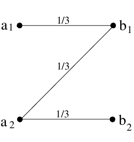
The graph G=(V,E,t)G=(V,E,t) associated with Figure 3 is shown in Figure 4. The graph has four vertices and three edges, each of them with weight 1/31/3.

Refer to caption
Figure 4: The graph associated with Figure 3.
Example 2.

For a more complicated example we consider a situation with p=2p=2 starting points and q=4q=4 ending points as in Figure 5.

Refer to caption
Figure 5: Non-intersecting Brownian motions with two starting points and four ending points, as discussed in Example 2.

The matrix of transition numbers is

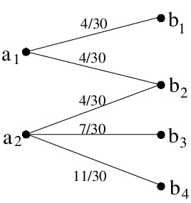
(tk,l)k=1,2,l=1,…,4=(4/304/300004/307/3011/30)\displaystyle\begin{pmatrix}t_{k,l}\end{pmatrix}_{k=1,2,\ l=1,\ldots,4}=\begin{pmatrix}4/30&4/30&0&0\\ 0&4/30&7/30&11/30\end{pmatrix} (2.8)

and the graph GG associated with (2.8) is shown in Figure 6.

Refer to caption
Figure 6: The graph associated with the transition numbers (2.8).

The constraints on the transition numbers are contained in the following obvious result that we state without proof.

Proposition 2.1.

The graph GG has the following properties:

  1. (a)

    GG has at most p+q−1p+q-1 edges. For each i=1,…,p+q−1i=1,\ldots,p+q-1, there is at most one non-vanishing transition number tk,lt_{k,l} with k+l−1=ik+l-1=i.

  2. (b)

    GG is a connected graph if and only if the number of edges is equal to p+q−1p+q-1.

  3. (c)

    GG has no cycles (and so GG is a tree if GG is connected).

In [10, 16] the special case of transition numbers

(tk,l)k=1,2,l=1,2=(1/2001/2)\left(t_{k,l}\right)_{k=1,2,\ l=1,2}=\begin{pmatrix}1/2&0\\ 0&1/2\end{pmatrix}

was considered. This example leads to a non-connected graph.

In the case of a connected graph the structure of the matrix of transition numbers (tk,l)(t_{k,l}) is easy to describe.

Proposition 2.2.

Suppose that the graph GG is connected. Then the non-zero entries of the matrix (tk,l)k,l\begin{pmatrix}t_{k,l}\end{pmatrix}_{k,l} are situated on a right-down path starting at the top left entry (1,1)(1,1) and ending at the bottom right entry (p,q)(p,q). The steps in the path are either by one unit to the right (a right step) or one unit down (a down step).

In Examples 1 and 2 we have

(×0××),(××000×××),\displaystyle\begin{pmatrix}\times&0\\ \times&\times\end{pmatrix},\qquad\begin{pmatrix}\times&\times&0&0\\ 0&\times&\times&\times\end{pmatrix},

respectively.

In this paper we consider only connected graphs, and we will make the following assumption.

Assumption 2.3.

We assume that the graph GG is connected. That is, we assume that GG has p+q−1p+q-1 edges, and for every i=1,…,p+q−1i=1,\ldots,p+q-1 there is exactly one non-vanishing transition number tk,lt_{k,l} with k+l−1=ik+l-1=i, and we define

k(i)=k,l(i)=l,if tk,l>0,andk+l−1=i.k(i)=k,\qquad l(i)=l,\qquad\text{if }t_{k,l}>0,\quad\text{and}\quad k+l-1=i.

It follows from the assumption and from (2.5) that also for large enough nn, the finite nn transition numbers have the same non-zero pattern. Thus tk,l(n)>0t_{k,l}^{(n)}>0 if and only if tk,l>0t_{k,l}>0.

In what follows we follow the convention that ii labels the edges EE of the graph, and so we identify ii with the edge

(ak⁡(i),bl⁡(i))(a_{k(i)},b_{l(i)})

of the graph.

2.2 Non-intersecting Brownian motions

We consider Brownian motions having transition probability density

P⁡(t,x,y)=12​π​t​σ2​e−12​t​σ2​(x−y)2P(t,x,y)=\frac{1}{\sqrt{2\pi t\sigma^{2}}}e^{-\frac{1}{2t\sigma^{2}}(x-y)^{2}} (2.9)

whose overall variance

σ2=Tn\sigma^{2}=\frac{T}{n} (2.10)

is proportional to 1/n1/n where nn is the number of Brownian paths. We interpret the proportionality constant T>0T>0 as a temperature variable.

In this paper we consider small temperature TT. We show that for small TT the paths at time tt have a limiting mean distribution that is characterized by a vector equilibrium problem. In the first theorem we state the existence of a limiting mean distribution.

Theorem 2.4.

Consider nn independent Brownian motions with transition probability (2.9)–(2.10) conditioned so that

  • •

    the paths are non-intersecting in the time interval (0,1)(0,1),

  • •

    nk,ln_{k,l} of the paths start at aka_{k} and end at blb_{l}, for each k=1,…,pk=1,\ldots,p and l=1,…,ql=1,\ldots,q.

Assume that as n→∞n\to\infty, the finite nn transition numbers nk,l/nn_{k,l}/n converge to tk,lt_{k,l}, and that the corresponding graph GG is connected.

Let t∈(0,1)t\in(0,1). Then there exists a T∗=T∗​(t)>0T^{*}=T^{*}(t)>0 so that for all T∈(0,T∗)T\in(0,T^{*}) the limiting mean distribution of the positions of the paths at time tt exists, and is supported on the union of p+q−1p+q-1 disjoint intervals ⋃i=1p+q−1[αi,βi]\bigcup_{i=1}^{p+q-1}[\alpha_{i},\beta_{i}] with a density ρi\rho_{i} on the iith interval.

The vector of measures (μ1,…,μp+q−1)(\mu_{1},\ldots,\mu_{p+q-1}) where d​μi​(x)=ρi​(x)​d​xd\mu_{i}(x)=\rho_{i}(x)dx for i=1,…,p+q−1i=1,\ldots,p+q-1 is the minimizer of a vector equilibrium problem that will be described in the next subsection.

The proof of Theorem 2.4 will be based on a Deift-Zhou steepest descent analysis of the Riemann-Hilbert problem in Section 2.5. The details of the steepest descent analysis will be described in Sections 5–7, and the proof of Theorem 2.4 will then be given in Section 8.

Remark 2.5.

The special case where p=1p=1, q=2q=2 and m1=m2=n/2m_{1}=m_{2}=n/2 was studied in [3, 5, 6]. In [5] the energy functional (2.15) is given for this special case, but it was not used in the further analysis. Instead the results in [5] were stated and proved in terms of an algebraic curve (Pastur’s equation).

Remark 2.6.

As already mentioned, for the case p=1p=1 and q≥2q\geq 2 the non-intersecting Brownian motions are distributed like the eigenvalues of the Gaussian unitary ensemble with external source.

There are more general random matrix ensembles with external source, which however do not have an equivalent interpretation in terms of non-intersecting paths. The case of a quartic potential was studied in [25]. An analogue of Theorem 2.4 is valid in this case as well, provided that a suitable analogue of the temperature TT is sufficiently small.

Note that Theorem 2.4 gives only a result for TT sufficiently small, but it does not specify how small TT should be. We expect that the theorem remains valid for all temperatures TT that are such that at time tt we have the maximal number of groups of paths. At a critical temperature Tcrit​(t)T_{\textrm{crit}}(t) we expect that two (or maybe more) neighboring intervals [αi,βi][\alpha_{i},\beta_{i}] and [αi+1,βi+1][\alpha_{i+1},\beta_{i+1}] merge and a Pearcey phase transition occurs. However we were unable to prove this.

2.3 Equilibrium problem

The logarithmic energy of a measure μ\mu on ℝ\mathbb{R} is defined as usual by

I⁡(μ)=∬log⁡1|x−y|​𝑑μ​(x)​𝑑μ​(y).I(\mu)=\iint\log\frac{1}{|x-y|}\,d\mu(x)\,d\mu(y). (2.11)

The mutual energy of two measures μ\mu, ν\nu is defined by

I⁡(μ,ν)=∬log⁡1|x−y|​𝑑μ​(x)​𝑑ν​(y).I(\mu,\nu)=\iint\log\frac{1}{|x-y|}\,d\mu(x)\,d\nu(y). (2.12)

We write for i=1,…,p+q−1i=1,\ldots,p+q-1,

xi​(t)=(1−t)​ak⁡(i)+t​bl⁡(i),0<t<1x_{i}(t)=(1-t)a_{k(i)}+tb_{l(i)},\qquad 0<t<1 (2.13)

and given t∈(0,1)t\in(0,1) we define the quadratic functions

Vi​(x)=12​t​(1−t)​(x−xi​(t))2,x∈ℝ,V_{i}(x)=\frac{1}{2t(1-t)}(x-x_{i}(t))^{2},\qquad x\in\mathbb{R}, (2.14)

for i=1,…,p+q−1i=1,\ldots,p+q-1. These functions will play the role of external fields in the vector equilibrium problem that is relevant for our problem.

Definition 2.7.

Fix t∈(0,1)t\in(0,1) and let T>0T>0. Consider the energy functional

E⁡(μ1,…,μp+q−1)=∑i,j=1p+q−1ai,j​I​(μi,μj)+1T​∑i=1p+q−1∫Vi​(x)​d​μi​(x),E(\mu_{1},\ldots,\mu_{p+q-1})=\sum_{i,j=1}^{p+q-1}a_{i,j}I(\mu_{i},\mu_{j})+\frac{1}{T}\sum_{i=1}^{p+q-1}\int V_{i}(x)\,d\mu_{i}(x), (2.15)

where ViV_{i} is defined in (2.14), and the interaction matrix A=(ai,j)A=(a_{i,j}) has entries

ai,j={1 if ​i=j,12 if ​i≠j​ and ​k​(i)=k⁡(j)​ or ​l​(i)=l⁡(j),0 otherwise.a_{i,j}=\left\{\begin{array}[]{ll}1&\textrm{ if }i=j,\\[5.0pt] \frac{1}{2}&\textrm{ if }i\neq j\textrm{ and }k(i)=k(j)\textrm{ or }l(i)=l(j),\\[5.0pt] 0&\textrm{ otherwise.}\end{array}\right. (2.16)

Then the vector equilibrium problem consists in minimizing the energy functional (2.15) over all vectors of positive measures (μ1,…,μp+q−1)(\mu_{1},\ldots,\mu_{p+q-1}) supported on the real line for which

∫dμi=tk⁡(i),l⁡(i),for i=1,…,p+q−1.\int d\mu_{i}=t_{k(i),l(i)},\qquad\text{for }i=1,\ldots,p+q-1. (2.17)

One may understand the energy minimization problem in Definition 2.7 as follows. To each of the edges of the graph G=(V,E,t)G=(V,E,t) we associate a measure μi\mu_{i}, i=1,…,p+q−1i=1,\ldots,p+q-1, of total mass equal to the weight tk⁡(i),l⁡(i)t_{k(i),l(i)} of that edge. This measure represents a distribution of charged particles on the real line that repel each other due to the diagonal term

ai,i​I​(μi,μi)=I⁡(μi,μi)a_{i,i}I(\mu_{i},\mu_{i})=I(\mu_{i},\mu_{i})

in (2.15). For the particles of different measures μi\mu_{i}, μj\mu_{j}, i≠ji\neq j, there are two possibilities. The first case is when the (i,j)(i,j) entry of (2.16) equals 1/21/2. This happens if the edges corresponding to ii and jj are adjacent in the graph GG. Then there is repulsion between the measures μi\mu_{i} and μj\mu_{j} but with a strength that is only half as strong as the repulsion for each individual measure. The second case is when the (i,j)(i,j) entry of (2.16) equals zero. In that case there is no direct interaction between the measures μi\mu_{i} and μj\mu_{j}.

The last term of (2.15) is a sum of external field terms due to the action of the external field 1T​Vi​(x)\frac{1}{T}V_{i}(x) on the measure μi\mu_{i}. The energy minimizer (μ1,…,μp+q−1)(\mu_{1},\ldots,\mu_{p+q-1}) in Definition 2.7 then corresponds to the equilibrium distribution of charged particles under the energy functional (2.15).

Proposition 2.8.

The interaction matrix AA is positive definite.

Proof.

It is easy to check that the interaction matrix AA is equal to

A=12​BT​BA=\frac{1}{2}B^{T}\,B (2.18)

where BB is the incidence matrix of the graph GG. That is, we choose a numbering k=1,…,p+qk=1,\ldots,p+q of the vertices, and then we have

B=(bk,i)k=1,…,p+q,i=1,…,p+q−1B=(b_{k,i})_{k=1,\ldots,p+q,\,i=1,\ldots,p+q-1}

where bk,i=1b_{k,i}=1 if vertex kk is incident to edge ii, and 00 otherwise.

From (2.18) we get that AA is positive semi-definite, and for any column vector 𝐱\mathbf{x} of length p+q−1p+q-1 we have

𝐱T​A​𝐱=12​‖B​𝐱‖2≥0.\mathbf{x}^{T}A\mathbf{x}=\frac{1}{2}\|B\mathbf{x}\|^{2}\geq 0. (2.19)

Now assume that B​𝐱=𝟎B\mathbf{x}=\mathbf{0}. Consider a leaf of GG, i.e., a vertex which is incident to exactly one edge. Then BB has exactly one zero in the row corresponding to this vertex, and from B​𝐱=𝟎B\mathbf{x}=\mathbf{0} it follows that the component of 𝐱\mathbf{x} corresponding to the edge that is incident to the leaf vanishes. Since GG is a tree (see Proposition 2.1(c)) we can then gradually undress GG by peeling off leafs one by one and we conclude in this way that all components of 𝐱\mathbf{x} are equal to 00. Thus 𝐱=𝟎\mathbf{x}=\mathbf{0} if B​𝐱=𝟎B\mathbf{x}=\mathbf{0}, which implies in view of (2.19) that AA is positive definite. ∎

Corollary 2.9.

The vector equilibrium problem of Definition 2.7 has a unique solution (μ1,…,μp+q−1)(\mu_{1},\ldots,\mu_{p+q-1}) and each measure μi\mu_{i} is compactly supported.

Proof.

The interaction matrix is positive definite by Proposition 2.8. The external fields ViV_{i} in the energy functional (2.15) have enough increase at ±∞\pm\infty so that standard arguments of potential theory as in [11, 27, 30] can be used to establish the existence and uniqueness of the minimizer as well as the fact that each measure μi\mu_{i} is supported on a compact set. ∎

Our next theorem describes the structure of the solution of the vector equilibrium problem for small TT.

Theorem 2.10.

Fix t∈(0,1)t\in(0,1), and let (tk,l)(t_{k,l}) be a matrix of transition numbers. Then there exists T∗>0T^{*}>0 (the same T∗T^{*} that makes Theorem 2.4 work) so that for every T∈(0,T∗)T\in(0,T^{*}) the following holds.

  • (a)

    Each μi\mu_{i} is supported on an interval

    supp(μi)=[αi,βi],i=1,…,p+q−1.\mathrm{supp}(\mu_{i})=[\alpha_{i},\beta_{i}],\qquad i=1,\ldots,p+q-1.

    The intervals [αi,βi][\alpha_{i},\beta_{i}] are pairwise disjoint and satisfy

    βi+1<αi,i=1,…,p+q−2.\beta_{i+1}<\alpha_{i},\qquad i=1,\ldots,p+q-2. (2.20)
  • (b)

    The measure μi\mu_{i} has a density ρi\rho_{i} with respect to Lebesgue measure which is real analytic and positive in the open interval (αi,βi)(\alpha_{i},\beta_{i}) and vanishes like a square root at the endpoints of [αi,βi][\alpha_{i},\beta_{i}], i.e., there exist non-zero constants ρi(1)\rho_{i}^{(1)} and ρi(2)\rho_{i}^{(2)} such that

    ρi​(x)=ρi(1)​x−αi+O⁡((x−αi)3/2)\displaystyle\rho_{i}(x)=\rho_{i}^{(1)}\sqrt{x-\alpha_{i}}+O((x-\alpha_{i})^{3/2})  as ​x↓αi,\displaystyle\quad\textrm{ as }x\downarrow\alpha_{i}, (2.21)
    ρi​(x)=ρi(2)​βi−x+O⁡((βi−x)3/2)\displaystyle\rho_{i}(x)=\rho_{i}^{(2)}\sqrt{\beta_{i}-x}+O((\beta_{i}-x)^{3/2})  as ​x↑βi.\displaystyle\quad\textrm{ as }x\uparrow\beta_{i}. (2.22)

The proof of Theorem 2.10 will be given in Section 3.1.

2.4 Special cases

In Subsections 2.4.1–2.4.3, our main Theorem 2.4 will be illustrated for some special cases.

2.4.1 The case p=1p=1: Angelesco-type interaction

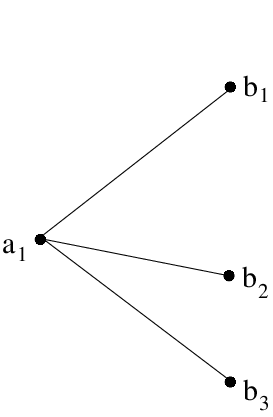
For the case p=1p=1 of one starting point, and an arbitrary number qq of ending points, the graph GG has a single vertex a1a_{1} on the left which is connected to each of the vertices b1,…,bqb_{1},\ldots,b_{q} on the right. For example, if q=3q=3 the graph has the form shown in Figure 7.
Refer to caption
Figure 7: A graph GG with p=1p=1 starting points and q=3q=3 ending points.

The energy functional (2.15)–(2.16) is then equal to

E⁡(μ1,…,μp+q−1):=∑i=1p+q−1I⁡(μi)+12​∑i≠jI⁡(μi,μj)+1T​∑i=1p+q−1∫Vi​(x)​d​μi​(x).E(\mu_{1},\ldots,\mu_{p+q-1}):=\sum_{i=1}^{p+q-1}I(\mu_{i})+\frac{1}{2}\sum_{i\neq j}I(\mu_{i},\mu_{j})+\frac{1}{T}\sum_{i=1}^{p+q-1}\int V_{i}(x)\,d\mu_{i}(x). (2.23)

The functional (2.23) is exactly the one familiar from the theory of Angelesco systems [21]. All off-diagonal entries in the interaction matrix AA in (2.16) are equal to 1/21/2. For the example in Figure 7 the interaction matrix is

A=(11/21/21/211/21/21/21).A=\begin{pmatrix}1&1/2&1/2\\ 1/2&1&1/2\\ 1/2&1/2&1\\ \end{pmatrix}. (2.24)

2.4.2 The ‘zigzag’ case: nearest neighbor interaction

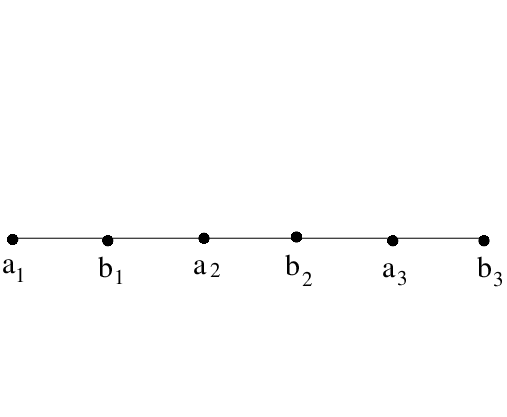
Next we consider the case where p=qp=q and the corresponding lattice path follows a zigzag line. The graph GG is then just a chain of vertices: see Figure 8.
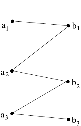
Refer to caption
Refer to caption
Figure 8: For p=q=3p=q=3, Figure 8 shows a graph GG which has zigzag form. Figure 8 shows the same graph written as a chain.

The energy functional (2.15) now takes the form

E⁡(μ1,…,μp+q−1):=∑i=1p+q−1I⁡(μi)+∑i=1p+q−2I⁡(μi,μi+1)+1T​∑i=1p+q−1∫Vi​(x)​d​μi​(x).E(\mu_{1},\ldots,\mu_{p+q-1}):=\sum_{i=1}^{p+q-1}I(\mu_{i})+\sum_{i=1}^{p+q-2}I(\mu_{i},\mu_{i+1})+\frac{1}{T}\sum_{i=1}^{p+q-1}\int V_{i}(x)\,d\mu_{i}(x). (2.25)

We see that the interaction matrix of (2.25) is tridiagonal with diagonal entries equal to 11, and entries on the first sub- and superdiagonal equal to 1/21/2. For the example in Figure 8 the interaction matrix equals

A=(11/20001/211/20001/211/20001/211/20001/21).A=\begin{pmatrix}1&1/2&0&0&0\\ 1/2&1&1/2&0&0\\ 0&1/2&1&1/2&0\\ 0&0&1/2&1&1/2\\ 0&0&0&1/2&1\\ \end{pmatrix}. (2.26)

Note that the tridiagonal structure of the interaction matrix means that there is only nearest neighbor interaction. The neighboring measures repel each other, since all signs in the interaction matrix are positive.

In a Nikishin system the interaction matrix is also tridiagonal, but the off-diagonal entries are −1/2-1/2 instead of 1/21/2, see [21].

2.4.3 The general case: block nearest neighbor interaction with Angelesco-type blocks

Finally we consider the graph GG in Figure 6. In this case the interaction matrix equals

A=(11/20001/211/20001/211/21/2001/211/2001/21/21).A=\begin{pmatrix}1&1/2&0&0&0\\ 1/2&1&1/2&0&0\\ 0&1/2&1&1/2&1/2\\ 0&0&1/2&1&1/2\\ 0&0&1/2&1/2&1\end{pmatrix}. (2.27)

Note that this interaction matrix is a mixture of the nearest neighbor and Angelesco interaction matrices. More precisely one could say that (2.27) has ‘block’ nearest neighbor interaction, where each of the blocks in turn has an Angelesco-type interaction, and with subsequent blocks intersecting in exactly one entry. For the matrix in (2.27) these building blocks are

(11/21/21),(11/21/21),(11/21/21/211/21/21/21).\begin{pmatrix}1&1/2\\ 1/2&1\end{pmatrix},\quad\begin{pmatrix}1&1/2\\ 1/2&1\end{pmatrix},\quad\begin{pmatrix}1&1/2&1/2\\ 1/2&1&1/2\\ 1/2&1/2&1\end{pmatrix}.

2.4.4 Comparison with [21]

A graph-based vector equilibrium problem was also considered in the work of Gonchar, Rakhmanov, and Sorokin [21]. The rule for building the interaction matrix from a graph GG is similar to the one in this paper. The vector equilibrium problem is also labeled by the edges of a graph, which in [21], however, is a directed rooted tree. The off-diagonal entries of the interaction matrix are non-zero if the corresponding two edges have a common vertex. The entry is 1/21/2 if the two edges have a common initial vertex, and −1/2-1/2 if the final vertex of one edge agrees with the initial vector of the other.

In our case, we only have 1/21/2 since the latter situation cannot happen.

2.5 About the proof of Theorem 2.4

The proof of Theorem 2.4 uses the connection of non-intersecting Brownian motions with prescribed starting and ending points with a determinantal point process and an associated Riemann-Hilbert problem. We recall this connection.

2.5.1 Determinantal point process

The positions at time t∈(0,1)t\in(0,1) of nn non-intersecting Brownian motions, starting at distinct aja_{j}, j=1,…,nj=1,\ldots,n, and ending at distinct positions bjb_{j}, j=1,…,nj=1,\ldots,n, have the joint probability density function

1Z​det(P⁡(t,ai,xj))i,j=1n⋅det(P⁡(1−t,xi,bj))i,j=1n,\frac{1}{Z}\det\left(P(t,a_{i},x_{j})\right)_{i,j=1}^{n}\cdot\det\left(P(1-t,x_{i},b_{j})\right)_{i,j=1}^{n},

with the transition probability density PP defined in (2.9) and with ZZ a normalization constant. This is a consequence of a theorem of Karlin and McGregor [23]. (For applications of the discrete version of the Karlin-McGregor theorem see e.g. [22].) In the confluent limit where nkn_{k} of the starting positions come together at aka_{k}, k=1,…,pk=1,\ldots,p, and mlm_{l} of the ending positions come together at blb_{l} for l=1,…,ql=1,\ldots,q, the joint p.d.f. for the positions of the paths at time tt can be written as

𝒫⁡(x1,…,xn)=1Z~​det(fi​(xj))i,j=1n⋅det(gi​(xj))i,j=1n,\mathcal{P}(x_{1},\ldots,x_{n})=\frac{1}{\tilde{Z}}\det\left(f_{i}(x_{j})\right)_{i,j=1}^{n}\cdot\det\left(g_{i}(x_{j})\right)_{i,j=1}^{n}, (2.28)

for certain functions fif_{i}, gig_{i}, that are built out of the p+qp+q functions

w1,k​(x)\displaystyle w_{1,k}(x) =e−12​t​σ2​(x−ak)2,k=1,…,p,\displaystyle=e^{-\frac{1}{2t\sigma^{2}}(x-a_{k})^{2}},\quad k=1,\ldots,p, (2.29)
w2,l​(x)\displaystyle w_{2,l}(x) =e−12​(1−t)​σ2​(x−bl)2,l=1,…,q,\displaystyle=e^{-\frac{1}{2(1-t)\sigma^{2}}(x-b_{l})^{2}},\quad l=1,\ldots,q, (2.30)

see e.g. [9].

The p.d.f. (2.28) defines a determinantal point process (in fact a biorthogonal ensemble, see [7]) with a correlation kernel K⁡(x,y)K(x,y) that is such that

𝒫⁡(x1,…,xn)=1n!​det(K⁡(xi,xj))i,j=1n\mathcal{P}(x_{1},\ldots,x_{n})=\frac{1}{n!}\det\left(K(x_{i},x_{j})\right)_{i,j=1}^{n} (2.31)

and for each m=1,…,nm=1,\ldots,n,

∫⋯∫𝒫(x1,…,xn)dxm+1⋯dxn=(n−m)!n!det(K(xi,xj))i,j=1m.\int\cdots\int\mathcal{P}(x_{1},\ldots,x_{n})\,dx_{m+1}\cdots dx_{n}=\frac{(n-m)!}{n!}\det\left(K(x_{i},x_{j})\right)_{i,j=1}^{m}. (2.32)

In particular for m=1m=1, we have that

1n​K​(x,x)\frac{1}{n}K(x,x)

is the mean density of paths.

2.5.2 Riemann-Hilbert problem

The kernel KK can be described in terms of the following Riemann-Hilbert problem (RH problem) introduced in [9].

RH problem 2.11.

The RH problem consists in finding a matrix-valued function Y:ℂ∖ℝ→ℂ(p+q)×(p+q)Y:\mathbb{C}\setminus\mathbb{R}\to\mathbb{C}^{(p+q)\times(p+q)} such that

  • (1)

    YY is analytic in ℂ∖ℝ\mathbb{C}\setminus\mathbb{R};

  • (2)

    For x∈ℝx\in\mathbb{R}, the limiting values

    Y+​(x)=limz→x,Im​z>0Y⁡(z),Y−​(x)=limz→x,Im​z<0Y⁡(z)Y_{+}(x)=\lim_{z\to x,\,\mathrm{Im}\,z>0}Y(z),\qquad Y_{-}(x)=\lim_{z\to x,\,\mathrm{Im}\,z<0}Y(z)

    exist and satisfy

    Y+​(x)=Y−​(x)​(IpW⁡(x)0Iq),Y_{+}(x)=Y_{-}(x)\begin{pmatrix}I_{p}&W(x)\\ 0&I_{q}\end{pmatrix}, (2.33)

    where IkI_{k} denotes the identity matrix of size kk, and where W⁡(x)W(x) denotes the rank-one matrix (outer product of two vectors)

    W⁡(x)=(w1,1​(x)w1,p​(x))​(w2,1​(x)⋯w2,q​(x))W(x)=\begin{pmatrix}w_{1,1}(x)\\ \vdots\\ w_{1,p}(x)\end{pmatrix}\begin{pmatrix}w_{2,1}(x)&\cdots&w_{2,q}(x)\end{pmatrix} (2.34)

    with w1,k​(x)w_{1,k}(x), k=1,…,pk=1,\ldots,p, and w2,l​(x)w_{2,l}(x), l=1,…,ql=1,\ldots,q given by (2.29) and (2.30).

  • (3)

    As z→∞z\to\infty, we have that

    Y⁡(z)=(Ip+q+O⁡(1/z))​diag⁡(zn1,…,znp,z−m1,…,z−mq).Y(z)=(I_{p+q}+O(1/z))\diag\left(z^{n_{1}},\ldots,z^{n_{p}},z^{-m_{1}},\ldots,z^{-m_{q}}\right). (2.35)

The RH problem has a unique solution that can be described in terms of multiple Hermite polynomials. This is shown in [9], generalizing results in [19, 32]. According to [9] the correlation kernel is expressed in terms of the solution to the RH problem as

K⁡(x,y)=12​π​i​(x−y)​(0⋯0w2,1​(y)…w2,q​(y))​Y+−1​(y)​Y+​(x)​(w1,1​(x)w1,p​(x)00).K(x,y)=\frac{1}{2\pi i(x-y)}\begin{pmatrix}0&\cdots&0&w_{2,1}(y)&\ldots&w_{2,q}(y)\end{pmatrix}Y_{+}^{-1}(y)Y_{+}(x)\begin{pmatrix}w_{1,1}(x)\\ \vdots\\ w_{1,p}(x)\\ 0\\ \vdots\\ 0\end{pmatrix}. (2.36)

It is also worth noticing that if Y1,1​(z)Y_{1,1}(z) denotes the top leftmost pp by pp block of the RH matrix Y⁡(z)Y(z), then the determinant of Y1,1​(z)Y_{1,1}(z) equals the average characteristic polynomial

detY1,1​(z)=𝔼⁡[∏j=1n(z−xj)],\det Y_{1,1}(z)=\mathbb{E}\left[\prod_{j=1}^{n}(z-x_{j})\right],

where the expectation 𝔼\mathbb{E} is taken according to the joint probability density (2.28). This was shown in [4] for the case p=1p=1 and in [15] for the case of general pp and qq.

2.5.3 Asymptotic analysis

We analyze the RH problem 2.11 in the limit described in Theorem 2.4. That is, we take σ2=T/n\sigma^{2}=T/n and we let nk→∞n_{k}\to\infty, ml→∞m_{l}\to\infty, so that

nk,ln→tk,las ​n→∞.\frac{n_{k,l}}{n}\to t_{k,l}\qquad\text{as }n\to\infty.

If, for each nn, we denote the correlation kernel (2.36) by KnK_{n}, then the limiting density of paths is

ρ⁡(x)=limn→∞1n​Kn​(x,x),x∈ℝ.\rho(x)=\lim_{n\to\infty}\frac{1}{n}K_{n}(x,x),\qquad x\in\mathbb{R}. (2.37)

The proof of Theorem 2.4 will be based on a steepest descent analysis of the RH problem 2.11. As a byproduct of this analysis we can also show that the local scaling limits of the limiting distribution of the Brownian motions are those familiar from random matrix theory, i.e., they are described in terms of the sine kernel in the bulk and the Airy kernel at the edge. We will not discuss this any further and refer to the papers [5, 6, 10, 28] for a more detailed analysis in a similar context.

2.6 Outline of the rest of the paper

The rest of this paper is organized as follows. In Section 3 we establish general properties of the equilibrium problem, in particular leading to the proof of Theorem 2.10. In Section 4 we define the ξ\xi-functions, λ\lambda-functions and the associated Riemann surface. These functions are used in Section 5 to normalize the RH problem at infinity. In Section 6 we apply Gaussian elimination to the RH problem by opening global lenses, thereby making the RH problem locally of size 2×22\times 2. This construction is fully systematic and may have interest in its own right. The remaining steps of the RH steepest descent analysis are described in Section 7. Finally, in Section 8 we prove the main Theorem 2.4.

3 Properties of the equilibrium measures

In this section we study the vector equilibrium problem of Definition 2.7. In particular we prove Theorem 2.10.

3.1 Proof of Theorem 2.10

The main difficulty is in the proof of part (a) of Theorem 2.10. For this we use the following lemma. Recall that t∈(0,1)t\in(0,1) is fixed.

Lemma 3.1.

For every ε>0\varepsilon>0 and τ>0\tau>0, there exists Tε>0T_{\varepsilon}>0 so that for every T∈(0,Tε)T\in(0,T_{\varepsilon}) the following holds.

If (μ1,…,μp+q−1)(\mu_{1},\ldots,\mu_{p+q-1}) is the minimizer for the energy functional (2.15) under the normalization (2.17) with

mini⁡tk⁡(i),l⁡(i)≥τ>0,\min_{i}t_{k(i),l(i)}\geq\tau>0, (3.1)

then the support of μi\mu_{i} is contained in [xi​(t)−ε,xi​(t)+ε][x_{i}(t)-\varepsilon,x_{i}(t)+\varepsilon] for every i=1,…,p+q−1i=1,\ldots,p+q-1.

Proof.

We are going to prove the following upper and lower bounds for the quantity

E∗:=E⁡(μ1,…,μp+q−1)E^{*}:=E(\mu_{1},\ldots,\mu_{p+q-1})

(which depends on the chosen normalization (2.17)).

  1. (a)

    There exist constants C1>0C_{1}>0 and C2,δC_{2,\delta} such that for every δ>0\delta>0 and T>0T>0 we have

    E∗≤C2,δ+C1​δ2T.E^{*}\leq C_{2,\delta}+C_{1}\frac{\delta^{2}}{T}. (3.2)

    The constant C1C_{1} is independent of δ\delta and TT, and C2,δC_{2,\delta} is independent of TT.

  2. (b)

    There exist positive constants C3C_{3}, and C4C_{4}, such that for every T∈(0,1]T\in(0,1] and every i=1,…,p+q−1i=1,\ldots,p+q-1, we have

    E∗≥−C3+C4T​(x−xi​(t))2,for ​x∈supp⁡(μi).E^{*}\geq-C_{3}+\frac{C_{4}}{T}(x-x_{i}(t))^{2},\qquad\text{for }x\in\mathrm{supp}(\mu_{i}). (3.3)

In addition, all constants C1C_{1}, C2,δC_{2,\delta}, C3C_{3} and C4C_{4} can be taken independently of the normalization (2.17), and only C4C_{4} depends on τ\tau.

Proof of (a):

We may assume that δ>0\delta>0 is sufficiently small so that

mini⁡(xi​(t)−xi+1​(t))≥2​δ.\min_{i}\left(x_{i}(t)-x_{i+1}(t)\right)\geq 2\delta.

Then the intervals [xi​(t)−δ,xi​(t)+δ][x_{i}(t)-\delta,x_{i}(t)+\delta] are mutually disjoint.

We fix transition numbers tk⁡(i),l⁡(i)≥0t_{k(i),l(i)}\geq 0 so that ∑itk⁡(i),l⁡(i)=1\sum_{i}t_{k(i),l(i)}=1. On each of the intervals [xi​(t)−δ,xi​(t)+δ][x_{i}(t)-\delta,x_{i}(t)+\delta] we choose a measure λi\lambda_{i} of finite energy with total mass 11 (for example, an appropriately rescaled and centered semi-circle law will do) and we put νi=tk⁡(i),l⁡(i)​λi\nu_{i}=t_{k(i),l(i)}\lambda_{i}. We choose the measures νi\nu_{i} independent of TT and so

∑i,j=1p+q−1ai,j​I​(νi,νj)\sum_{i,j=1}^{p+q-1}a_{i,j}I(\nu_{i},\nu_{j}) (3.4)

does not depend on TT. The sum (3.4) depends continuously on the numbers tk⁡(i),l⁡(i)t_{k(i),l(i)} and so

C2,δ=max∑i,j=1p+q−1ai,jI(νi,νj)C_{2,\delta}=\max\sum_{i,j=1}^{p+q-1}a_{i,j}I(\nu_{i},\nu_{j}) (3.5)

exists, where the maximum is taken over all choices tk⁡(i),l⁡(i)≥0t_{k(i),l(i)}\geq 0 with ∑itk⁡(i),l⁡(i)=1\sum_{i}t_{k(i),l(i)}=1.

Since Vi​(x)≤δ22​t​(1−t)V_{i}(x)\leq\frac{\delta^{2}}{2t(1-t)} on [xi​(t)−δ,xi​(t)+δ][x_{i}(t)-\delta,x_{i}(t)+\delta], we also have

∫Vi​(x)​d​νi​(x)≤δ22​t​(1−t)\int V_{i}(x)d\nu_{i}(x)\leq\frac{\delta^{2}}{2t(1-t)}

and

∑i=1p+q−1∫Vi​(x)​d​νi​(x)≤C1​δ2\sum_{i=1}^{p+q-1}\int V_{i}(x)\,d\nu_{i}(x)\leq C_{1}\delta^{2} (3.6)

with a constant C1C_{1} that is independent of TT and δ\delta, and also of the tk⁡(i),l⁡(i)t_{k(i),l(i)}. Then part (a) follows from (3.5), (3.6), and the fact that

E∗≤E⁡(ν1,…,νp+q−1)=∑i,j=1p+q−1ai,j​I​(νi,νj)+1T​∑i=1p+q−1∫Vi​(x)​d​νi​(x).E^{*}\leq E(\nu_{1},\ldots,\nu_{p+q-1})=\sum_{i,j=1}^{p+q-1}a_{i,j}I(\nu_{i},\nu_{j})+\frac{1}{T}\sum_{i=1}^{p+q-1}\int V_{i}(x)d\nu_{i}(x).
Proof of (b):

For each ii we take a measure νi\nu_{i} of total mass ‖νi‖=‖μi‖\|\nu_{i}\|=\|\mu_{i}\| and satisfying for some constant K≥1K\geq 1,

νi≤Kμi,for i=1,…,p+q−1.\nu_{i}\leq K\mu_{i},\qquad\text{for }i=1,\ldots,p+q-1. (3.7)

Then (1−λ)​μi+λ​νi(1-\lambda)\mu_{i}+\lambda\nu_{i} is a positive measure for every λ∈[−1/K,1]\lambda\in[-1/K,1], and so

E∗≤E⁡((1−λ)​μ1+λ​ν1,…,(1−λ)​μp+q−1+λ​νp+q−1)E^{*}\leq E\left((1-\lambda)\mu_{1}+\lambda\nu_{1},\ldots,(1-\lambda)\mu_{p+q-1}+\lambda\nu_{p+q-1}\right) (3.8)

for every λ∈[−1/K,1]\lambda\in[-1/K,1], with equality for λ=0\lambda=0. Thus the λ\lambda-derivative of the right-hand side of (3.8) vanishes for λ=0\lambda=0, which leads to

E∗=∑i,j=1p+q−1ai,j​I​(μi,νj)+12​T​∑i=1p+q−1∫Vi​(x)​(d​μi​(x)+d​νi​(x)).E^{*}=\sum_{i,j=1}^{p+q-1}a_{i,j}I(\mu_{i},\nu_{j})+\frac{1}{2T}\sum_{i=1}^{p+q-1}\int V_{i}(x)\,\left(d\mu_{i}(x)+d\nu_{i}(x)\right). (3.9)

From the elementary inequality |x−y|≤x2+1​y2+1|x-y|\leq\sqrt{x^{2}+1}\sqrt{y^{2}+1} it follows that

I⁡(μi,νj)\displaystyle I(\mu_{i},\nu_{j}) =∬log⁡1|x−y|​d​μi​(x)​d​νj​(y)\displaystyle=\iint\log\frac{1}{|x-y|}d\mu_{i}(x)d\nu_{j}(y)
≥−12∬log(x2+1)dμi(x)dνj(y)−12∬log(y2+1)dμi(x)dνj(y)\displaystyle\geq-\frac{1}{2}\iint\log(x^{2}+1)d\mu_{i}(x)d\nu_{j}(y)-\frac{1}{2}\iint\log(y^{2}+1)d\mu_{i}(x)d\nu_{j}(y)
≥−12∫log(x2+1)(dμi(x)+dνj(x))\displaystyle\geq-\frac{1}{2}\int\log(x^{2}+1)\left(d\mu_{i}(x)+d\nu_{j}(x)\right)

where for the last inequality we used the facts that log⁡(x2+1)≥0\log(x^{2}+1)\geq 0 and ‖νj‖≤1\|\nu_{j}\|\leq 1, ‖μi‖≤1\|\mu_{i}\|\leq 1. Since all ai,j≥0a_{i,j}\geq 0 it then follows from (3.9) that

E∗\displaystyle E^{*} ≥−12∑i,j=1p+q−1ai,j∫log(x2+1)(dμi(x)+dνj(x))+12​T∑i=1p+q−1∫Vi(x)(dμi(x)+dνi(x))\displaystyle\geq-\frac{1}{2}\sum_{i,j=1}^{p+q-1}a_{i,j}\int\log(x^{2}+1)\left(d\mu_{i}(x)+d\nu_{j}(x)\right)+\frac{1}{2T}\sum_{i=1}^{p+q-1}\int V_{i}(x)\left(d\mu_{i}(x)+d\nu_{i}(x)\right)
=12​T​∑i=1p+q−1∫(Vi​(x)−T​∑j=1p+q−1ai,j​log⁡(x2+1))​(d​μi​(x)+d​νi​(x)).\displaystyle=\frac{1}{2T}\sum_{i=1}^{p+q-1}\int\left(V_{i}(x)-T\sum_{j=1}^{p+q-1}a_{i,j}\log(x^{2}+1)\right)\,(d\mu_{i}(x)+d\nu_{i}(x)). (3.10)

For i=1,…,p+q−1i=1,\ldots,p+q-1 and T≤1T\leq 1, the functions Vi​(x)−T​∑j=1p+q−1ai,j​log⁡(x2+1)V_{i}(x)-T\sum_{j=1}^{p+q-1}a_{i,j}\log(x^{2}+1) are bounded from below and assume their minimum value in a fixed compact interval (independent of ii and T≤1T\leq 1). This is clear from the explicit form (2.14) of the functions ViV_{i}, and from the fact that ∑j=1p+q−1ai,j≤p+q2\sum_{j=1}^{p+q-1}a_{i,j}\leq\frac{p+q}{2} for each ii. Thus

Vi​(x)−T​∑j=1p+q−1ai,j​log⁡(x2+1)≥12​Vi​(x)−C0​T≥−C0​T,x∈ℝ,V_{i}(x)-T\sum_{j=1}^{p+q-1}a_{i,j}\log(x^{2}+1)\geq\frac{1}{2}V_{i}(x)-C_{0}T\geq-C_{0}T,\qquad x\in\mathbb{R},

for some constant C0>0C_{0}>0 independent of T≤1T\leq 1 and ii.

Using this in (3.10) we find that for each i=1,…,p+q−1i=1,\ldots,p+q-1,

E∗≥−C3+14​T​∫Vi​(x)​d​νi​(x),E^{*}\geq-C_{3}+\frac{1}{4T}\int V_{i}(x)\,d\nu_{i}(x), (3.11)

where C3>0C_{3}>0 is a constant independent of ii and T≤1T\leq 1. The inequality (3.11) (with the same constant C3C_{3}) holds for all measures νi\nu_{i} with ‖νi‖=tk⁡(i),l⁡(i)\|\nu_{i}\|=t_{k(i),l(i)} and satisfying (3.7) for some KK. For every xx in the support of μi\mu_{i}, we can approximate the point mass ‖μi‖​δx\|\mu_{i}\|\,\delta_{x} by such νi\nu_{i}. It thus follows from (3.11) that

E∗≥−C3+14​T​Vi​(x)​tk⁡(i),l⁡(i),for ​x∈supp⁡(μi).E^{*}\geq-C_{3}+\frac{1}{4T}V_{i}(x)\,t_{k(i),l(i)},\qquad\textrm{for }x\in\mathrm{supp}(\mu_{i}).

If tk⁡(i),l⁡(i)≥τt_{k(i),l(i)}\geq\tau as in (3.1), then we obtain (3.3) with

C4=14⋅12​t​(1−t)⋅τ.C_{4}=\frac{1}{4}\cdot\frac{1}{2t(1-t)}\cdot\tau.
Conclusion of the proof:

Combining (3.2) and (3.3) we find that there exist positive constants C5=C1/C4C_{5}=C_{1}/C_{4} and C6,δ=(C2,δ+C3)/C4C_{6,\delta}=(C_{2,\delta}+C_{3})/C_{4} so that

(x−xi​(t))2≤C5​δ2+C6,δ​T,for ​x∈supp⁡(μi),(x-x_{i}(t))^{2}\leq C_{5}\delta^{2}+C_{6,\delta}T,\qquad\text{for }x\in\mathrm{supp}(\mu_{i}),

for every i=1,…,p+q−1i=1,\ldots,p+q-1, T≤1T\leq 1 and δ>0\delta>0.

Let ε>0\varepsilon>0 be given. Choose first δ>0\delta>0 so that C5​δ2≤12​ε2C_{5}\delta^{2}\leq\frac{1}{2}\varepsilon^{2} and then choose Tε∈(0,1]T_{\varepsilon}\in(0,1] so that C6,δ​Tε≤12​ε2C_{6,\delta}T_{\varepsilon}\leq\frac{1}{2}\varepsilon^{2}. Then for every i=1,…,p+q−1i=1,\ldots,p+q-1 and T≤TεT\leq T_{\varepsilon},

(x−xi​(t))2≤ε2,for ​x∈supp⁡(μi),(x-x_{i}(t))^{2}\leq\varepsilon^{2},\qquad\text{for }x\in\mathrm{supp}(\mu_{i}),

and Lemma 3.1 follows. ∎

Having Lemma 3.1 the proof of Theorem 2.10 is rather straightforward.

Proof.

(Proof of Theorem 2.10)

(a) Let ε>0\varepsilon>0 be such that the intervals [xi​(t)−ε,xi​(t)+ε][x_{i}(t)-\varepsilon,x_{i}(t)+\varepsilon], i=1,…,p+q−1i=1,\ldots,p+q-1, are disjoint. From Lemma 3.1 we know that there exists Tϵ>0T_{\epsilon}>0 so that for T<TεT<T_{\varepsilon} the support of μi\mu_{i} is contained in [xi​(t)−ε,xi​(t)+ε][x_{i}(t)-\varepsilon,x_{i}(t)+\varepsilon].

Take i=1,…,p+q−1i=1,\ldots,p+q-1, and fix the other measures μj\mu_{j}, j≠ij\neq i. From (2.12), (2.15) we see that the measure μi\mu_{i} is the equilibrium measure in an effective external field

∑j≠iai,j​∫log⁡1|x−y|​d​μj​(y)+1T​Vi​(x),\sum_{j\neq i}a_{i,j}\int\log\frac{1}{|x-y|}\,d\mu_{j}(y)+\frac{1}{T}V_{i}(x), (3.12)

and it is also the minimizer if we restrict to measures with total mass tk⁡(i),l⁡(i)t_{k(i),l(i)} that are supported on [xi​(t)−ε,xi​(t)+ε][x_{i}(t)-\varepsilon,x_{i}(t)+\varepsilon]. On this interval the external field (3.12) is strictly convex (we use that the measures μj\mu_{j} with j≠ij\neq i are supported outside [xi​(t)−ε,xi​(t)+ε][x_{i}(t)-\varepsilon,x_{i}(t)+\varepsilon]). The convexity implies that the support of μi\mu_{i} is an interval, see e.g. [30, Theorem IV 1.10].

(b) The real analyticity of the density of μi\mu_{i} in the interior of the support follows from [12], since the effective external field (3.12) is real analytic on the support of μi\mu_{i}.

The convexity of (3.12) implies that the density of μi\mu_{i} does not vanish in the interior of the support, and has square root behavior at the endpoints, see e.g. [8, Lemma 3.5]. ∎

3.2 Varying nn

In the situation of Theorem 2.4 we have for each finite nn, the number nk,ln_{k,l} of paths going from aka_{k} to blb_{l}. The finite nn transition numbers are

tk,l(n)=nk,lnt_{k,l}^{(n)}=\frac{n_{k,l}}{n}

and in the limit we have

limn→∞tk,l(n)=tk,lfor ​k=1,…,p,l=1,…,q.\lim_{n\to\infty}t_{k,l}^{(n)}=t_{k,l}\qquad\textrm{for }k=1,\ldots,p,\,l=1,\ldots,q. (3.13)

The equilibrium problem depends on the transition numbers by means of the normalizations (2.17). For a finite nn, we use the equilibrium problem for a vector of measures (μ1,…,μp+q−1)(\mu_{1},\ldots,\mu_{p+q-1}) that have total masses

∫dμi=tk⁡(i),l⁡(i)(n),for i=1,…,p+q−1\int d\mu_{i}=t_{k(i),l(i)}^{(n)},\qquad\textrm{for }i=1,\ldots,p+q-1 (3.14)

instead of (2.17). Then the minimizer (μ1(n),…,μp+q−1(n))(\mu_{1}^{(n)},\ldots,\mu_{p+q-1}^{(n)}) will also depend on nn.

Because of Theorem 2.10 and (3.13), there is a T0>0T_{0}>0, so that for every T<T0T<T_{0}, each μi(n)\mu_{i}^{(n)} is supported on an interval [αi(n),βi(n)][\alpha_{i}^{(n)},\beta_{i}^{(n)}] (depending on nn) so that parts (a) and (b) of Theorem 2.10 hold. As n→∞n\to\infty, we have that μi(n)→μi\mu_{i}^{(n)}\to\mu_{i} and

αi(n)→αi,βi(n)→βi.\alpha_{i}^{(n)}\to\alpha_{i},\qquad\beta_{i}^{(n)}\to\beta_{i}.

for every ii.

In the steepest descent analysis that follows we will fix a large enough nn. We will work with the nn-dependent measures μi(n)\mu_{i}^{(n)} and intervals [αi(n),βi(n)][\alpha_{i}^{(n)},\beta_{i}^{(n)}], but for ease of notation we will usually not write the superscript (n)(n). We trust that this will not lead to confusion. However, we will write tk,l(n)t_{k,l}^{(n)}. A property that will be used a number of times is that

n​tk,l(n)=nk,lis an integer.nt_{k,l}^{(n)}=n_{k,l}\qquad\textrm{is an integer.} (3.15)

4 Riemann surface, ξ\xi-functions, λ\lambda-functions

4.1 Variational conditions

As said before, we take a large nn and consider the vector equilibrium problem with normalization (3.14) and we assume that TT is sufficiently small so that Theorem 2.10 applies. So the measure μi\mu_{i} is supported on the interval [αi,βi][\alpha_{i},\beta_{i}].

The variational conditions associated with the vector equilibrium problem (2.15) are as follows. For each i=1,…,p+q−1i=1,\ldots,p+q-1, there is a constant Li∈ℝL_{i}\in\mathbb{R} so that

2​∑jai,j​∫log⁡1|x−y|​d​μj​(y)+1T​Vi​(x)​{=Li,x∈[αi,βi],≥Li,x∈ℝ∖[αi,βi].2\sum_{j}a_{i,j}\int\log\frac{1}{|x-y|}\,d\mu_{j}(y)+\frac{1}{T}V_{i}(x)\left\{\begin{array}[]{l}=L_{i},\quad x\in[\alpha_{i},\beta_{i}],\\ \geq L_{i},\quad x\in\mathbb{R}\setminus[\alpha_{i},\beta_{i}].\end{array}\right. (4.1)

We use FiF_{i} to denote the Cauchy transform of the measure μi\mu_{i},

Fi​(z):=∫αiβi1z−x​d​μi​(x),F_{i}(z):=\int_{\alpha_{i}}^{\beta_{i}}\frac{1}{z-x}\,d\mu_{i}(x), (4.2)

for i=1,…,p+q−1i=1,\ldots,p+q-1. The function Fi​(z)F_{i}(z) is analytic on ℂ∖[αi,βi]\mathbb{C}\setminus[\alpha_{i},\beta_{i}]. By taking the derivative of (4.1) and using the Sokhotski-Plemelj formula it follows that

−Fi,+​(x)−Fi,−​(x)−2​∑j≠iai,j​Fj​(x)+1T​Vi′​(x)=0,x∈[αi,βi].-F_{i,+}(x)-F_{i,-}(x)-2\sum_{j\neq i}a_{i,j}F_{j}(x)+\frac{1}{T}V_{i}^{\prime}(x)=0,\quad x\in[\alpha_{i},\beta_{i}]. (4.3)
Lemma 4.1.

The variational inequality (4.1) is strict for x∈[βi+1,αi)∪(βi,αi−1]x\in[\beta_{i+1},\alpha_{i})\cup(\beta_{i},\alpha_{i-1}], where we put α0=+∞\alpha_{0}=+\infty and βp+q=−∞\beta_{p+q}=-\infty.

Proof.

On both gaps (βi+1,αi)(\beta_{i+1},\alpha_{i}) and (βi,αi−1)(\beta_{i},\alpha_{i-1}), the left-hand side of (4.1) is a real analytic function of xx whose first derivative is

−2∑jai,jFj(x)+1TVi′(x)-2\sum_{j}a_{i,j}F_{j}(x)+\frac{1}{T}V_{i}^{\prime}(x) (4.4)

and whose second derivative is

2​∑jai,j​∫αiβi1(x−y)2​d​μj​(y)+1T​Vi′′​(x).2\sum_{j}a_{i,j}\int_{\alpha_{i}}^{\beta_{i}}\frac{1}{(x-y)^{2}}\,d\mu_{j}(y)+\frac{1}{T}V_{i}^{\prime\prime}(x). (4.5)

Each term in (4.5) is positive and so the left-hand side of (4.1) is strictly convex on both (βi+1,αi)(\beta_{i+1},\alpha_{i}) and (βi,αi−1)(\beta_{i},\alpha_{i-1}), which proves the lemma. ∎

4.2 Riemann surface

We construct a Riemann surface ℛ\mathcal{R} as follows, compare with [17]. The Riemann surface has p+qp+q sheets which we denote by ℛj\mathcal{R}_{j}, j=1,…,p+qj=1,\ldots,p+q. Each sheet is associated with a vertex of the graph, that is, with either a starting point aka_{k} or an ending point blb_{l}. We choose the numbering so that ℛk\mathcal{R}_{k} is associated with aka_{k} for k=1,…,pk=1,\ldots,p, and ℛp+l\mathcal{R}_{p+l} is associated with blb_{l} for l=1,…,ql=1,\ldots,q.

Recall that we use ii as a label for the edges of the graph, and we write k=k⁡(i)k=k(i) and l=l⁡(i)l=l(i) if ii labels the edge (ak,bl)(a_{k},b_{l}). Then the p+qp+q sheets are defined as

ℛk\displaystyle\mathcal{R}_{k} =ℂ¯∖⋃i:k⁡(i)=k[αi,βi],k=1,…,p,\displaystyle=\overline{\mathbb{C}}\setminus\bigcup_{i:\,k(i)=k}[\alpha_{i},\beta_{i}],\quad k=1,\ldots,p, (4.6)
ℛp+l\displaystyle\mathcal{R}_{p+l} =ℂ¯∖⋃i:l⁡(i)=l[αi,βi],l=1,…,q.\displaystyle=\overline{\mathbb{C}}\setminus\bigcup_{i:\,l(i)=l}[\alpha_{i},\beta_{i}],\quad l=1,\ldots,q. (4.7)

The sheets are connected as follows. For each i=1,…,p+q−1i=1,\ldots,p+q-1 we have that ℛk⁡(i)\mathcal{R}_{k(i)} is connected to sheet ℛp+l⁡(i)\mathcal{R}_{p+l(i)} along the interval [αi,βi][\alpha_{i},\beta_{i}] in the usual crosswise manner. See Figure 9 for a picture of the Riemann surface for the example in Figure 4. Note that the cuts [αi,βi][\alpha_{i},\beta_{i}] are always between a sheet ℛk\mathcal{R}_{k} which is among the first pp sheets and a sheet ℛp+l\mathcal{R}_{p+l} which is among the last qq sheets. The cuts strictly move to the left if we go from one sheet to the next among the first pp sheets, and similarly, among the last qq sheets.

The Riemann surface depends on nn, since the endpoints αi(n)\alpha_{i}^{(n)} and βi(n)\beta_{i}^{(n)} depend on nn. The ξ\xi- and λ\lambda-functions that we define from the Riemann surface will also depend on nn. We will not indicate the nn-dependence, as already mentioned before.

α 1 β 1 ξ 1 α 3 β 3 α 2 β 2 ξ 2 α 2 β 2 α 1 β 1 ξ 3 α 3 β 3 ξ 4
Figure 9: Four-sheeted Riemann surface for the example in Figure 4.

The Riemann surface ℛ\mathcal{R} has p+qp+q sheets and 2​(p+q−1)2(p+q-1) simple branch points. Therefore by Hurwitz’s formula (see e.g. [26]) its genus gg satisfies

2​g−2=−2​(p+q)+2​(p+q−1)=−22g-2=-2(p+q)+2(p+q-1)=-2

so that g=0g=0. The fact that the genus is zero will be helpful in the construction of the global parametrix in Section 7.2.

4.3 ξ\xi-functions

We define the ξ\xi-functions as follows. Recall that FiF_{i} is given by (4.2).

ξk​(z)\displaystyle\xi_{k}(z) =−∑i:k⁡(i)=kFi(z)+1T​t(z−ak),\displaystyle=-\sum_{i:\,k(i)=k}F_{i}(z)+\frac{1}{Tt}(z-a_{k}), k=1,…,p,\displaystyle k=1,\ldots,p, (4.8)
ξp+l​(z)\displaystyle\xi_{p+l}(z) =∑i:l⁡(i)=lFi(z)−1T⁡(1−t)(z−bl),\displaystyle=\sum_{i:\,l(i)=l}F_{i}(z)-\frac{1}{T(1-t)}(z-b_{l}), l=1,…,q.\displaystyle l=1,\ldots,q. (4.9)

We consider ξj\xi_{j} as an analytic function on the jjth sheet ℛj\mathcal{R}_{j} of the Riemann surface with a pole at infinity. Moreover, these functions define a global meromorphic function on ℛ\mathcal{R} as the following result shows.

Theorem 4.2.

Consider the function ξj​(z)\xi_{j}(z) on the jjth sheet ℛj\mathcal{R}_{j}, j=1,…,p+qj=1,\ldots,p+q. Then these functions are compatible along the cuts [αi,βi][\alpha_{i},\beta_{i}] of the Riemann surface in the sense that

{ξk⁡(i),+​(x)=ξp+l⁡(i),−​(x),ξk⁡(i),−​(x)=ξp+l⁡(i),+​(x),x∈[αi,βi],\left\{\begin{array}[]{l}\xi_{k(i),+}(x)=\xi_{p+l(i),-}(x),\\ \xi_{k(i),-}(x)=\xi_{p+l(i),+}(x),\end{array}\right.\quad x\in[\alpha_{i},\beta_{i}], (4.10)

for every i=1,…,p+q−1i=1,\ldots,p+q-1. Hence the ξj\xi_{j}-functions can be extended to a global meromorphic function ξ\xi defined on the Riemann surface ℛ\mathcal{R}.

Proof.

Fix i∈{1,…,p+q−1}i\in\{1,\ldots,p+q-1\}. On the interval [αi,βi][\alpha_{i},\beta_{i}] we have by definition (4.8)–(4.9) that

ξk⁡(i),+​(x)−ξp+l⁡(i),−​(x)=−∑j:k⁡(j)=k⁡(i)Fj,+(x)−∑j:l⁡(j)=l⁡(i)Fj,−(x)+1T​t​(1−t)(x−(1−t)ak⁡(i)−tbl⁡(i)))=−Fi,+(x)−Fi,−(x)−(∑j≠i:k⁡(j)=k⁡(i)​ or ​l​(j)=l⁡(i)Fj(x))+1TV′i(x),\xi_{k(i),+}(x)-\xi_{p+l(i),-}(x)\\ =-\sum_{j:\,k(j)=k(i)}F_{j,+}(x)-\sum_{j:\,l(j)=l(i)}F_{j,-}(x)+\frac{1}{Tt(1-t)}(x-(1-t)a_{k(i)}-tb_{l(i)}))\\ =-F_{i,+}(x)-F_{i,-}(x)-\left(\sum_{j\neq i:\,k(j)=k(i)\textrm{ or }l(j)=l(i)}F_{j}(x)\right)+\frac{1}{T}V^{\prime}_{i}(x), (4.11)

where we used the definition (2.13)–(2.14) of ViV_{i}.

If j≠ij\neq i is such that k⁡(j)=k⁡(i)k(j)=k(i) or l⁡(j)=l⁡(i)l(j)=l(i) then ai,j=1/2a_{i,j}=1/2. For all other j≠ij\neq i we have ai,j=0a_{i,j}=0. Therefore

(∑j≠i:k⁡(j)=k⁡(i)​ or ​l​(j)=l⁡(i)Fj(x))=2∑j≠iai,jFj(x).\left(\sum_{j\neq i:\,k(j)=k(i)\textrm{ or }l(j)=l(i)}F_{j}(x)\right)=2\sum_{j\neq i}a_{i,j}F_{j}(x).

Using this in (4.11) and recalling the variational equality (4.3), we see that that ξk⁡(i),+​(x)=ξp+l⁡(i),−​(x)\xi_{k(i),+}(x)=\xi_{p+l(i),-}(x) for x∈[αi,βi]x\in[\alpha_{i},\beta_{i}].

The other equality ξk⁡(i),−​(x)=ξp+l⁡(i),+​(x)\xi_{k(i),-}(x)=\xi_{p+l(i),+}(x) follows in exactly the same way. ∎

In the following two lemmas we collect some more properties of the ξ\xi-functions that will be needed in what follows.

Lemma 4.3.

The ξ\xi-functions have the following behavior as z→∞z\to\infty

ξk​(z)\displaystyle\xi_{k}(z) =1T​t(z−ak)−nkn​z+O(1z2),k=1,…,p,\displaystyle=\frac{1}{Tt}(z-a_{k})-\frac{n_{k}}{nz}+O\left(\frac{1}{z^{2}}\right),\qquad k=1,\ldots,p, (4.12)
ξp+l​(z)\displaystyle\xi_{p+l}(z) =−1T⁡(1−t)(z−bl)+mln​z+O(1z2),l=1,…,q.\displaystyle=-\frac{1}{T(1-t)}(z-b_{l})+\frac{m_{l}}{nz}+O\left(\frac{1}{z^{2}}\right),\qquad l=1,\ldots,q. (4.13)
Proof.

From (4.2) and (3.14) it follows that

Fi​(z)=∫d​μiz+O⁡(1z2)=tk⁡(i),l⁡(i)(n)z+O⁡(1z2)F_{i}(z)=\frac{\int d\mu_{i}}{z}+O\left(\frac{1}{z^{2}}\right)=\frac{t_{k(i),l(i)}^{(n)}}{z}+O\left(\frac{1}{z^{2}}\right) (4.14)

as z→∞z\to\infty. Recall that we work with nn-dependent transition numbers. Since

∑i:k⁡(i)=ktk⁡(i),l⁡(i)(n)=nkn,∑i:l⁡(i)=ltk⁡(i),l⁡(i)(n)=mln\sum_{i:\,k(i)=k}t_{k(i),l(i)}^{(n)}=\frac{n_{k}}{n},\qquad\sum_{i:\,l(i)=l}t_{k(i),l(i)}^{(n)}=\frac{m_{l}}{n}

the asymptotic behaviors (4.12) and (4.13) follow immediately from the definitions (4.8)–(4.9). ∎

Lemma 4.4.

For any i=1,…,p+q−1i=1,\ldots,p+q-1 we have

∫𝒞iξk⁡(i)​(z)​𝑑z\displaystyle\int_{\mathcal{C}_{i}}\xi_{k(i)}(z)\,dz =−2​π​i​tk⁡(i),l⁡(i)(n),\displaystyle=-2\pi{\rm i}\,t_{k(i),l(i)}^{(n)}, (4.15)
∫𝒞iξp+l⁡(i)​(z)​𝑑z\displaystyle\int_{\mathcal{C}_{i}}\xi_{p+l(i)}(z)\,dz =2​π​i​tk⁡(i),l⁡(i)(n),\displaystyle=2\pi{\rm i}\,t_{k(i),l(i)}^{(n)}, (4.16)
∫𝒞iξj​(z)​𝑑z\displaystyle\int_{\mathcal{C}_{i}}\xi_{j}(z)\,dz =0,j∉{k⁡(i),p+l⁡(i)},\displaystyle=0,\qquad\qquad j\not\in\{k(i),p+l(i)\}, (4.17)

where 𝒞i\mathcal{C}_{i} denotes a counterclockwise contour surrounding the interval [αi,βi][\alpha_{i},\beta_{i}] and not enclosing any point of the other intervals [αj,βj][\alpha_{j},\beta_{j}], j≠ij\neq i.

Proof.

From (4.2), (4.14) and the definition of 𝒞i\mathcal{C}_{i} it follows that

∫𝒞iFi​(z)​𝑑z=2​π​i​tk⁡(i),l⁡(i)(n)\int_{\mathcal{C}_{i}}F_{i}(z)\,dz=2\pi{\rm i}\,t_{k(i),l(i)}^{(n)}

and

∫𝒞iFj​(z)​𝑑z=0if ​j≠i.\int_{\mathcal{C}_{i}}F_{j}(z)\,dz=0\qquad\textrm{if }j\neq i.

The lemma then follows from the definitions (4.8)–(4.9). ∎

Remark 4.5.

Our definition of the ξ\xi-functions differs slightly from the one used in [5]. If ξ~j\tilde{\xi}_{j} denote the ξ\xi-functions in [5] then we have

ξj(z)=ξ~j(z)−zT⁡(1−t),j=1,…,p+q.\xi_{j}(z)=\tilde{\xi}_{j}(z)-\frac{z}{T(1-t)},\qquad j=1,\ldots,p+q.

In the present form the formulae are more symmetric.

4.4 λ\lambda-functions

We define the λj\lambda_{j}-functions as

λk​(z)\displaystyle\lambda_{k}(z) =ck+∫βikzξk​(s)​𝑑s,\displaystyle=c_{k}+\int_{\beta_{i_{k}}}^{z}\xi_{k}(s)\,ds, k=1,…,p,\displaystyle k=1,\ldots,p, (4.18)
λp+l​(z)\displaystyle\lambda_{p+l}(z) =cp+l+∫βi~lzξp+l​(s)​𝑑s,\displaystyle=c_{p+l}+\int_{\beta_{\tilde{i}_{l}}}^{z}\xi_{p+l}(s)\,ds, l=1,…,q,\displaystyle l=1,\ldots,q, (4.19)

where

ik:=min⁡{i∣k⁡(i)=k},andi~l:=min⁡{i∣l⁡(i)=l},i_{k}:=\min\{i\mid k(i)=k\},\quad\text{and}\quad\tilde{i}_{l}:=\min\{i\mid l(i)=l\},

and where the path of integration in the integrals (4.18) and (4.19) lies in ℂ∖(−∞,βik)\mathbb{C}\setminus(-\infty,\beta_{i_{k}}) and ℂ∖(−∞,βi~l)\mathbb{C}\setminus(-\infty,\beta_{\tilde{i}_{l}}), respectively. The functions λk​(z)\lambda_{k}(z) and λp+l​(z)\lambda_{p+l}(z) are defined with a branch cut along the intervals (−∞,βik](-\infty,\beta_{i_{k}}] and (−∞,βi~l](-\infty,\beta_{\tilde{i}_{l}}], respectively.

We choose the constants cjc_{j} in in the following way.

Lemma 4.6.

We can (and do) choose the constants cjc_{j} in (4.18)–(4.19) in such a way that

Re⁡(λk⁡(i),+​(βi))=Re⁡(λp+l⁡(i),+​(βi)),\mathrm{Re}\,(\lambda_{k(i),+}(\beta_{i}))=\mathrm{Re}\,(\lambda_{p+l(i),+}(\beta_{i})), (4.20)

for every i=1,…,p+q−1i=1,\ldots,p+q-1.

Proof.

We use the fact that the graph G=(V,E,t)G=(V,E,t) is a tree. We can iteratively ‘undress’ this tree as follows. We start with G1=GG_{1}=G. Next we choose a leaf vertex vv and set

G2=G1∖v,G_{2}=G_{1}\setminus v,

i.e., G2G_{2} is the tree obtained by removing the leaf and its corresponding edge from the tree G1G_{1}. We iteratively repeat this procedure and obtain in this way a chain of nested trees

G=G1⊃G2⊃⋯⊃G|V|,G=G_{1}\supset G_{2}\supset\cdots\supset G_{|V|}, (4.21)

where each GiG_{i} is obtained from Gi−1G_{i-1} by removing one leaf. Obviously the last non-empty tree G|V|G_{|V|} in this chain consists of a single vertex vjv_{j}.

We freely choose the corresponding constant cjc_{j}. Next we use induction on k=|V|−1,…,2,1k=|V|-1,\ldots,2,1, to fill in all the remaining constants cjc_{j} so that each time (4.20) is satisfied. This is possible since Gi−1∖GiG_{i-1}\setminus G_{i} consists of a single vertex vjv_{j}, which is a leaf of Gi−1G_{i-1}, and hence we have exactly one condition (4.20) to fix the integration constant cjc_{j} of this leaf. Thus we see that the conditions (4.20) can indeed be imposed on the constants cjc_{j} in (4.18)–(4.19). ∎

Properties of the λ\lambda-functions that we will need are stated in the following lemmas. The first is a reformulation of the variational conditions (4.1).

Lemma 4.7.

We have for i=1,…,p+q−1i=1,\ldots,p+q-1,

Re⁡(λk⁡(i),±​(x)−λp+l⁡(i),±​(x))​{=0,x∈[αi,βi],≥0,x∈ℝ∖[αi,βi].\mathrm{Re}\,(\lambda_{k(i),\pm}(x)-\lambda_{p+l(i),\pm}(x))\left\{\begin{array}[]{l}=0,\quad x\in[\alpha_{i},\beta_{i}],\\ \geq 0,\quad x\in\mathbb{R}\setminus[\alpha_{i},\beta_{i}].\end{array}\right. (4.22)

Strict inequality in (4.22) holds for x∈[βi+1,αi)∪(βi,αi−1]x\in[\beta_{i+1},\alpha_{i})\cup(\beta_{i},\alpha_{i-1}] (where α0=+∞\alpha_{0}=+\infty and βp+q=−∞\beta_{p+q}=-\infty).

Proof.

Observe that by (4.8)–(4.9) and (4.18)–(4.19) we have that

λk​(z)\displaystyle\lambda_{k}(z) =∑i:k⁡(i)=k∫log1z−xdμi(x)+12​T​t(z−ak)2+c~k,\displaystyle=\sum_{i:\,k(i)=k}\int\log\frac{1}{z-x}\,d\mu_{i}(x)+\frac{1}{2Tt}(z-a_{k})^{2}+\tilde{c}_{k}, (4.23)
λp+l​(z)\displaystyle\lambda_{p+l}(z) =−∑i:l⁡(i)=l∫log1z−xdμi(x)−12​T​(1−t)(z−bl)2+c~p+l,\displaystyle=-\sum_{i:\,l(i)=l}\int\log\frac{1}{z-x}\,d\mu_{i}(x)-\frac{1}{2T(1-t)}(z-b_{l})^{2}+\tilde{c}_{p+l}, (4.24)

for certain real constants c~j\tilde{c}_{j}, j=1,…,p+qj=1,\ldots,p+q. Therefore, for i=1,…,p+q−1i=1,\ldots,p+q-1,

Re⁡(λk⁡(i)​(z)−λp+l⁡(i)​(z))=2∫log1|z−x|dμi(x)+∑j≠i:k⁡(j)=k⁡(i)​ or ​l​(j)=l⁡(i)∫log1|z−x|dμj(x)+1T​Re​Vi​(z)+12​T​(ak⁡(i)−bl⁡(i))2+c~k⁡(i)−c~p+l⁡(i),\mathrm{Re}\,(\lambda_{k(i)}(z)-\lambda_{p+l(i)}(z))\\ =2\int\log\frac{1}{|z-x|}\,d\mu_{i}(x)+\sum_{j\neq i:\,k(j)=k(i)\textrm{ or }l(j)=l(i)}\int\log\frac{1}{|z-x|}\,d\mu_{j}(x)\\ +\frac{1}{T}\mathrm{Re}\,V_{i}(z)+\frac{1}{2T}(a_{k(i)}-b_{l(i)})^{2}+\tilde{c}_{k(i)}-\tilde{c}_{p+l(i)}, (4.25)

where we used the definition (2.14) of ViV_{i}. Then by the variational conditions (4.1) we have

Re⁡(λk⁡(i),±​(x)−λp+l⁡(i),±​(x))≥Li+12​T​(ak⁡(i)−bl⁡(i))2+c~k⁡(i)−c~p+l⁡(i)\mathrm{Re}\,(\lambda_{k(i),\pm}(x)-\lambda_{p+l(i),\pm}(x))\geq L_{i}+\frac{1}{2T}(a_{k(i)}-b_{l(i)})^{2}+\tilde{c}_{k(i)}-\tilde{c}_{p+l(i)} (4.26)

for x∈ℝx\in\mathbb{R} with equality for x∈[αi,βi]x\in[\alpha_{i},\beta_{i}]. The constant in the right-hand side of (4.26) is equal to zero because the constants cjc_{j} are chosen so that (4.20) holds.

The strict inequality for x∈[βi+1,αi)∪(βi,αi−1]x\in[\beta_{i+1},\alpha_{i})\cup(\beta_{i},\alpha_{i-1}] is a consequence of Lemma 4.1. ∎

Lemma 4.8.

As z→∞z\to\infty we have that

λk​(z)\displaystyle\lambda_{k}(z) =12​T​t(z−ak)2−nknlogz+c~k+O(1z),k=1,…,p,\displaystyle=\frac{1}{2Tt}(z-a_{k})^{2}-\frac{n_{k}}{n}\log z+\tilde{c}_{k}+O\left(\frac{1}{z}\right),\quad k=1,\ldots,p, (4.27)
λp+l​(z)\displaystyle\lambda_{p+l}(z) =−12​T​(1−t)(z−bl)2+mlnlogz+c~p+l+O(1z),l=1,…,q.\displaystyle=-\frac{1}{2T(1-t)}(z-b_{l})^{2}+\frac{m_{l}}{n}\log z+\tilde{c}_{p+l}+O\left(\frac{1}{z}\right),\quad l=1,\ldots,q. (4.28)
Proof.

This follows from the definitions (4.18) and (4.19) and the asymptotic behavior (4.12) and (4.13) of the ξ\xi-functions. ∎

The next lemma will be a consequence of Lemma 4.4.

Lemma 4.9.

For k=1,…,pk=1,\ldots,p, we have that

exp(n(λk,+(x)−λk,−(x)))=1,for x∈ℝ∖⋃i:k⁡(i)=k[αi,βi].\exp(n(\lambda_{k,+}(x)-\lambda_{k,-}(x)))=1,\qquad\textrm{for }x\in\mathbb{R}\setminus\bigcup_{i:\,k(i)=k}[\alpha_{i},\beta_{i}]. (4.29)

For l=1,…,ql=1,\ldots,q, we have that

exp(n(λp+l,+(x)−λp+l,−(x)))=1,for x∈ℝ∖⋃i:l⁡(i)=l[αi,βi].\exp(n(\lambda_{p+l,+}(x)-\lambda_{p+l,-}(x)))=1,\qquad\textrm{for }x\in\mathbb{R}\setminus\bigcup_{i:\,l(i)=l}[\alpha_{i},\beta_{i}]. (4.30)
Proof.

Fix k=1,…,pk=1,\ldots,p and let x∈ℝ∖⋃i:k⁡(i)=k[αi,βi]x\in\mathbb{R}\setminus\bigcup_{i:\,k(i)=k}[\alpha_{i},\beta_{i}]. By definition of λk\lambda_{k} and by contour deformation we have that

λk,+​(x)−λk,−​(x)=∫𝒞ξk​(z)​𝑑z\lambda_{k,+}(x)-\lambda_{k,-}(x)=\int_{\mathcal{C}}\xi_{k}(z)\,dz

where 𝒞\mathcal{C} is some closed contour surrounding some of the intervals [αi,βi][\alpha_{i},\beta_{i}]. From Lemma 4.4 it follows that each of the enclosed intervals gives a contribution to the integral of the form ±2​π​i​tk,l(n)\pm 2\pi{\rm i}\,t_{k,l}^{(n)}. Since each tk,l(n)t_{k,l}^{(n)} is a rational number with denominator nn, indeed tk,l(n)=nk,l/nt_{k,l}^{(n)}=n_{k,l}/n, we conclude that n⁡(λk,+​(x)−λk,−​(x))n(\lambda_{k,+}(x)-\lambda_{k,-}(x)) is a multiple of 2​π​i2\pi{\rm i}, and so we obtain (4.29).

The proof of (4.30) is similar. ∎

Lemma 4.9 will be important for the steepest descent analysis in Section 5.

5 First transformation of the RH problem: Normalization at infinity

In the following sections we describe the steepest descent analysis Y↦X↦T↦S↦RY\mapsto X\mapsto T\mapsto S\mapsto R of the RH problem 2.11. Throughout the steepest descent analysis the following simple lemma will be repeatedly used.

Lemma 5.1.

Assume that the matrix function Y⁡(z)Y(z) satisfies the jump condition Y+​(x)=Y−​(x)​J​(x)Y_{+}(x)=Y_{-}(x)J(x) for x∈ℝx\in\mathbb{R}. Let A⁡(z)A(z) and B⁡(z)B(z) be matrix functions with A⁡(z)A(z) entire and B⁡(z)B(z) analytic in ℂ∖ℝ\mathbb{C}\setminus\mathbb{R}. Then

X⁡(z):=A⁡(z)​Y​(z)​B​(z)X(z):=A(z)Y(z)B(z)

satisfies the jump condition

X+​(x)=X−​(x)​(B−−1​(x)​J​(x)​B+​(x)).X_{+}(x)=X_{-}(x)\left(B^{-1}_{-}(x)J(x)B_{+}(x)\right).

The point will be to choose appropriate transformation matrices A⁡(z)A(z) and B⁡(z)B(z) in order to bring the RH problem 2.11 to a simple form.

Let YY be the solution to the original RH problem 2.11. The first transformation Y↦XY\mapsto X serves to normalize the RH problem at infinity. To this end we define X=X⁡(z)X=X(z) as

X⁡(z)=L−n​Y​(z)​D​(z)n,X(z)=L^{-n}Y(z)D(z)^{n}, (5.1)

where we define the diagonal matrices

D(z)=diag((exp(λk(z)−12​T​t(z−ak)2))k=1p,OPEN(exp⁡(λp+l​(z)+12​T​(1−t)​(z−bl)2))l=1q),D(z)=\diag\left(\left(\exp\left(\lambda_{k}(z)-\frac{1}{2Tt}(z-a_{k})^{2}\right)\right)_{k=1}^{p},\right.\\ \left.\left(\exp\left(\lambda_{p+l}(z)+\frac{1}{2T(1-t)}(z-b_{l})^{2}\right)\right)_{l=1}^{q}\right), (5.2)

and

L=diag⁡(exp⁡(c~1),…,exp⁡(c~p+q)),L=\diag(\exp(\tilde{c}_{1}),\ldots,\exp(\tilde{c}_{p+q})), (5.3)

where the constants c~j\tilde{c}_{j} are as in (4.27)–(4.28). From Lemma 5.1 it follows by straightforward calculations that X=X⁡(z)X=X(z) satisfies the following RH problem.

RH problem 5.2.
  • (1)

    XX is analytic in ℂ∖ℝ\mathbb{C}\setminus\mathbb{R};

  • (2)

    For x∈ℝx\in\mathbb{R}, we have that

    X+​(x)=X−​(x)​(J1,1​(x)J1,2​(x)0J2,2​(x))X_{+}(x)=X_{-}(x)\begin{pmatrix}J_{1,1}(x)&J_{1,2}(x)\\ 0&J_{2,2}(x)\end{pmatrix} (5.4)

    where the blocks J1,1J_{1,1}, J1,2J_{1,2} and J2,2J_{2,2} (of sizes p×pp\times p, p×qp\times q and q×qq\times q, respectively) have the following form.

    1. (a)

      J1,2J_{1,2} is a full p×qp\times q matrix with entries

      (J1,2​(x))k,l=exp⁡(n⁡(λp+l,+​(x)−λk,−​(x))),x∈ℝ.\left(J_{1,2}(x)\right)_{k,l}=\exp\left(n(\lambda_{p+l,+}(x)-\lambda_{k,-}(x))\right),\qquad x\in\mathbb{R}. (5.5)
    2. (b)

      Outside of the intervals [αi,βi][\alpha_{i},\beta_{i}], J1,1J_{1,1} and J2,2J_{2,2} are identity matrices

      J1,1​(x)=Ip,J2,2​(x)=Iq,x∈ℝ∖⋃i=1p+q−1[αi,βi].J_{1,1}(x)=I_{p},\qquad J_{2,2}(x)=I_{q},\qquad x\in\mathbb{R}\setminus\bigcup_{i=1}^{p+q-1}[\alpha_{i},\beta_{i}]. (5.6)
    3. (c)

      On the interval [αi,βi][\alpha_{i},\beta_{i}], J1,1J_{1,1} and J2,2J_{2,2} are diagonal matrices with ones on the diagonal, except for

      (J1,1​(x))k⁡(i),k⁡(i)=exp⁡(n⁡(λk⁡(i),+​(x)−λk⁡(i),−​(x))),x∈(αi,βi),\left(J_{1,1}(x)\right)_{k(i),k(i)}=\exp\left(n(\lambda_{k(i),+}(x)-\lambda_{k(i),-}(x))\right),\qquad x\in(\alpha_{i},\beta_{i}),\\ (5.7)

      and

      (J2,2​(x))l⁡(i),l⁡(i)=exp⁡(n⁡(λp+l⁡(i),+​(x)−λp+l⁡(i),−​(x))),x∈(αi,βi).\left(J_{2,2}(x)\right)_{l(i),l(i)}=\exp\left(n(\lambda_{p+l(i),+}(x)-\lambda_{p+l(i),-}(x))\right),\qquad x\in(\alpha_{i},\beta_{i}). (5.8)
  • (3)

    As z→∞z\to\infty, we have that

    X⁡(z)=Ip+q+O⁡(1/z).X(z)=I_{p+q}+O(1/z). (5.9)

Here we used Lemma 4.9 to see that the diagonal entries of (5.6), as well as most of the diagonal entries of (5.7)–(5.8) are equal to 11. On the other hand, we used the asymptotic conditions (4.27)–(4.28) and (5.1)–(5.3) to see that the RH problem for XX is normalized at infinity in the sense of (5.9).

Let us illustrate the jump matrices for the example with p=q=2p=q=2 as in Figures 4 and 9. In that case the jump conditions are written as

X+=X−​(exp⁡(n⁡(λ1,+−λ1,−))0exp⁡(n⁡(λ3,+−λ1,−))exp⁡(n⁡(λ4−λ1,−))01exp⁡(n⁡(λ3,+−λ2))exp⁡(n⁡(λ4−λ2))00exp⁡(n⁡(λ3,+−λ3,−))00001)X_{+}=X_{-}\begin{pmatrix}\exp(n(\lambda_{1,+}-\lambda_{1,-}))&0&\exp(n(\lambda_{3,+}-\lambda_{1,-}))&\exp(n(\lambda_{4}-\lambda_{1,-}))\\ 0&1&\exp(n(\lambda_{3,+}-\lambda_{2\phantom{,-}}))&\exp(n(\lambda_{4}-\lambda_{2\phantom{,-}}))\\ 0&0&\exp(n(\lambda_{3,+}-\lambda_{3,-}))&0\\ 0&0&0&1\end{pmatrix}

on the interval [α1,β1][\alpha_{1},\beta_{1}],

X+=X−​(10exp⁡(n⁡(λ3,+−λ1))exp⁡(n⁡(λ4−λ1))0exp⁡(n⁡(λ2,+−λ2,−))exp⁡(n⁡(λ3,+−λ2,−))exp⁡(n⁡(λ4−λ2,−))00exp⁡(n⁡(λ3,+−λ3,−))00001)X_{+}=X_{-}\begin{pmatrix}1&0&\exp(n(\lambda_{3,+}-\lambda_{1\phantom{,-}}))&\exp(n(\lambda_{4}-\lambda_{1\phantom{,-}}))\\ 0&\exp(n(\lambda_{2,+}-\lambda_{2,-}))&\exp(n(\lambda_{3,+}-\lambda_{2,-}))&\exp(n(\lambda_{4}-\lambda_{2,-}))\\ 0&0&\exp(n(\lambda_{3,+}-\lambda_{3,-}))&0\\ 0&0&0&1\end{pmatrix}

on the interval [α2,β2][\alpha_{2},\beta_{2}],

X+=X−​(10exp⁡(n⁡(λ3−λ1))exp⁡(n⁡(λ4,+−λ1))0exp⁡(n⁡(λ2,+−λ2,−))exp⁡(n⁡(λ3−λ2,−))exp⁡(n⁡(λ4,+−λ2,−))0010000exp⁡(n⁡(λ4,+−λ4,−)))X_{+}=X_{-}\begin{pmatrix}1&0&\exp(n(\lambda_{3}-\lambda_{1\phantom{,-}}))&\exp(n(\lambda_{4,+}-\lambda_{1\phantom{,-}}))\\ 0&\exp(n(\lambda_{2,+}-\lambda_{2,-}))&\exp(n(\lambda_{3}-\lambda_{2,-}))&\exp(n(\lambda_{4,+}-\lambda_{2,-}))\\ 0&0&1&0\\ 0&0&0&\exp(n(\lambda_{4,+}-\lambda_{4,-}))\\ \end{pmatrix}

on the interval [α3,β3][\alpha_{3},\beta_{3}], and

X+=X−​(10exp⁡(n⁡(λ3−λ1))exp⁡(n⁡(λ4−λ1))01exp⁡(n⁡(λ3−λ2))exp⁡(n⁡(λ4−λ2))00100001)X_{+}=X_{-}\begin{pmatrix}1&0&\exp(n(\lambda_{3}-\lambda_{1}))&\exp(n(\lambda_{4}-\lambda_{1}))\\ 0&1&\exp(n(\lambda_{3}-\lambda_{2}))&\exp(n(\lambda_{4}-\lambda_{2}))\\ 0&0&1&0\\ 0&0&0&1\\ \end{pmatrix}

on ℝ∖⋃i=13[αi,βi]\mathbb{R}\setminus\bigcup_{i=1}^{3}[\alpha_{i},\beta_{i}].

6 Second transformation of the RH problem: Gaussian elimination and opening of global lenses

On the interval [αi,βi][\alpha_{i},\beta_{i}] we have that λp+l⁡(i),+−λk⁡(i),−\lambda_{p+l(i),+}-\lambda_{k(i),-} is a purely imaginary constant. So the entry

(J1,2​(x))k⁡(i),l⁡(i),x∈[αi,βi]\left(J_{1,2}(x)\right)_{k(i),l(i)},\qquad x\in[\alpha_{i},\beta_{i}] (6.1)

is constant with modulus one. It would be an ideal situation if, except for (6.1), all entries of the matrix J1,2​(x)J_{1,2}(x) for x∈ℝx\in\mathbb{R}, are exponentially decaying as n→∞n\to\infty. That would happen if for every k=1,…,pk=1,\ldots,p, and l=1,…,ql=1,\ldots,q, we have

  1. (a)

    if tk,l(n)=0t_{k,l}^{(n)}=0 then

    Re​λp+l,+​(x)<Re​λk,−​(x),x∈ℝ,\mathrm{Re}\,\lambda_{p+l,+}(x)<\mathrm{Re}\,\lambda_{k,-}(x),\qquad x\in\mathbb{R},
  2. (b)

    if tk,l(n)>0t_{k,l}^{(n)}>0 then

    Re​λp+l,+​(x)<Re​λk,−​(x),x∈ℝ∖[αi,βi],\mathrm{Re}\,\lambda_{p+l,+}(x)<\mathrm{Re}\,\lambda_{k,-}(x),\qquad x\in\mathbb{R}\setminus[\alpha_{i},\beta_{i}],

    where i=k+l−1i=k+l-1.

However, this will not happen in general, and that is why we need a second transformation X↦TX\mapsto T in the steepest descent analysis of the RH problem in which a number of unwanted entries of the jump matrices are eliminated. In particular those entries of J1,2​(x)J_{1,2}(x) that could potentially be exponentially increasing as n→∞n\to\infty.

To this end we will open global lenses [3] and apply Gaussian elimination inside each of the lenses. This construction will be systematic and may have interest in its own right. The proof that appropriate lenses exist will be a consequence of the maximum principle for subharmonic functions.

The opening of global lenses can be conveniently described in terms of the right-down path in Proposition 2.2. We start at the top left entry (1,1)(1,1) of the matrix of transition numbers (tk,l(n))(t_{k,l}^{(n)}) and walk along the path until we arrive at the bottom right entry (p,q)(p,q). During this walk, we will open global lenses in an appropriate way. The precise action to perform depends on whether we are taking a vertical (down) or a horizontal (right) step along the path.

6.1 Construction of global lenses: Vertical step

First we construct the global lenses for a vertical step along the lattice path. Thus assume that i∈{1,…,p+q−2}i\in\{1,\ldots,p+q-2\} is such that

(k⁡(i),l⁡(i))\displaystyle(k(i),l(i)) =(k,l),\displaystyle=(k,l), (6.2)
(k⁡(i+1),l⁡(i+1))\displaystyle(k(i+1),l(i+1)) =(k+1,l),\displaystyle=(k+1,l), (6.3)

for certain k=1,…,p−1k=1,\ldots,p-1 and l=1,…,ql=1,\ldots,q.

From (4.27) we obtain the asymptotic behavior

λk+1​(z)−λk​(z)=\displaystyle\lambda_{k+1}(z)-\lambda_{k}(z)= 1T​t​(ak−ak+1)​z+O⁡(log⁡|z|),\displaystyle\frac{1}{Tt}(a_{k}-a_{k+1})z+O(\log|z|), (6.4)

as z→∞z\to\infty.

We also note that Re​λk\mathrm{Re}\,\lambda_{k} and Re​λk+1\mathrm{Re}\,\lambda_{k+1} are well-defined and continuous on ℂ\mathbb{C}. Indeed, we have by (4.23) that

Re​(λk​(z))\displaystyle\mathrm{Re}\,(\lambda_{k}(z)) =∑j:k⁡(j)=k∫log1|z−x|dμj(x)+12​T​tRe(z−ak)2+c~k,\displaystyle=\sum_{j:\,k(j)=k}\int\log\frac{1}{|z-x|}d\mu_{j}(x)+\frac{1}{2Tt}\mathrm{Re}\,(z-a_{k})^{2}+\tilde{c}_{k}, (6.5)
Re​(λk+1​(z))\displaystyle\mathrm{Re}\,(\lambda_{k+1}(z)) =∑j:k⁡(j)=k+1∫log1|z−x|dμj(x)+12​T​tRe(z−ak+1)2+c~k+1,\displaystyle=\sum_{j:\,k(j)=k+1}\int\log\frac{1}{|z-x|}d\mu_{j}(x)+\frac{1}{2Tt}\mathrm{Re}\,(z-a_{k+1})^{2}+\tilde{c}_{k+1}, (6.6)

for certain constants c~k\tilde{c}_{k} and c~k+1\tilde{c}_{k+1}.

The representations (6.5) and (6.6) also show the following.

Lemma 6.1.

The function z↦Re⁡(λk+1​(z)−λk​(z))z\mapsto\mathrm{Re}\,(\lambda_{k+1}(z)-\lambda_{k}(z)) is superharmonic on ℂ∖⋃j:k⁡(j)=k[αj,βj]\mathbb{C}\setminus\bigcup_{j:\,k(j)=k}[\alpha_{j},\beta_{j}], and subharmonic on ℂ∖⋃j:k⁡(j)=k+1[αj,βj]\mathbb{C}\setminus\bigcup_{j:\,k(j)=k+1}[\alpha_{j},\beta_{j}].

Proof.

It is a standard fact from potential theory that any function of the form z↦∫log⁡1|z−x|​𝑑μ​(x)z\mapsto\int\log\frac{1}{|z-x|}\,d\mu(x), with μ\mu a positive measure with compact support, is superharmonic on ℂ\mathbb{C} and harmonic on ℂ∖supp⁡(μ)\mathbb{C}\setminus\mathrm{supp}(\mu), see e.g. [30, Chapter 0]. Thus by (6.5) and (6.6) we have that z↦Re​λk+1​(z)z\mapsto\mathrm{Re}\,\lambda_{k+1}(z) is superharmonic on ℂ\mathbb{C} and harmonic on ℂ∖⋃j:k⁡(j)=k+1[αj,βj]\mathbb{C}\setminus\bigcup_{j:\,k(j)=k+1}[\alpha_{j},\beta_{j}], while z↦−Re​λk​(z)z\mapsto-\mathrm{Re}\,\lambda_{k}(z) is subharmonic on ℂ\mathbb{C} and harmonic on ℂ∖⋃j:k⁡(j)=k[αj,βj]\mathbb{C}\setminus\bigcup_{j:\,k(j)=k}[\alpha_{j},\beta_{j}]

Since the two sets ⋃j:k⁡(j)=k[αj,βj]\bigcup_{j:\,k(j)=k}[\alpha_{j},\beta_{j}] and ⋃j:k⁡(j)=k+1[αj,βj]\bigcup_{j:\,k(j)=k+1}[\alpha_{j},\beta_{j}] are disjoint, the lemma follows. ∎

We next define the open sets Ω+,Ω−⊂ℂ\Omega_{+},\Omega_{-}\subset\mathbb{C} as follows

Ω+\displaystyle\Omega_{+} :={z∈ℂ∣Re⁡(λk+1​(z)−λk​(z))>0}\displaystyle:=\{z\in\mathbb{C}\mid\mathrm{Re}\,(\lambda_{k+1}(z)-\lambda_{k}(z))>0\} (6.7)
Ω−\displaystyle\Omega_{-} :={z∈ℂ∣Re⁡(λk+1​(z)−λk​(z))<0}.\displaystyle:=\{z\in\mathbb{C}\mid\mathrm{Re}\,(\lambda_{k+1}(z)-\lambda_{k}(z))<0\}. (6.8)

We also denote

Ω+,∞\displaystyle\Omega_{+,\infty} :={z∈Ω+∣∃ a connected path in Ω+ from z to ∞}\displaystyle:=\{z\in\Omega_{+}\mid\exists\textrm{ a connected path in $\Omega_{+}$ from $z$ to $\infty$}\} (6.9)
Ω−,∞\displaystyle\Omega_{-,\infty} :={z∈Ω−∣∃ a connected path in Ω− from z to ∞}.\displaystyle:=\{z\in\Omega_{-}\mid\exists\textrm{ a connected path in $\Omega_{-}$ from $z$ to $\infty$}\}. (6.10)

In other words, Ω+,∞\Omega_{+,\infty} is the union of the unbounded connected components of Ω+\Omega_{+}, and similarly for Ω−,∞\Omega_{-,\infty}.

The open sets Ω+,∞\Omega_{+,\infty}, Ω−,∞\Omega_{-,\infty} satisfy the following properties.

Lemma 6.2.
  1. (a)

    For each ε>0\varepsilon>0 there exists R>0R>0 so that

    {z∈ℂ∣|z|>R,−π/2+ε<argz<π/2−ε}\displaystyle\{z\in\mathbb{C}\mid|z|>R,\,-\pi/2+\varepsilon<\arg z<\pi/2-\varepsilon\} ⊂Ω+,∞,\displaystyle\subset\Omega_{+,\infty}, (6.11)

    and

    {z∈ℂ∣|z|>R,π/2+ε<argz<3π/2−ε}\displaystyle\{z\in\mathbb{C}\mid|z|>R,\,\pi/2+\varepsilon<\arg z<3\pi/2-\varepsilon\} ⊂Ω−,∞.\displaystyle\subset\Omega_{-,\infty}. (6.12)

    In particular, Ω+,∞\Omega_{+,\infty} lies to the right of Ω−,∞\Omega_{-,\infty}.

  2. (b)

    Both Ω+,∞\Omega_{+,\infty} and Ω−,∞\Omega_{-,\infty} are connected.

Proof.

Part (a) follows from (6.4) and the the fact that ak>ak+1a_{k}>a_{k+1}. Part (b) follows from part (a) in a similar way as in [16, Proof of Lemma 2.4], to which we refer for further details. ∎

Lemma 6.3.

We have

αi∈Ω+,∞andβi+1∈Ω−,∞,\displaystyle\alpha_{i}\in\Omega_{+,\infty}\qquad\text{and}\qquad\beta_{i+1}\in\Omega_{-,\infty}, (6.13)

where we recall ii is related to kk as in (6.2) and (6.3).

Proof.

By applying the variational conditions (4.22) twice, first with the index ii and then with i+1i+1, we obtain

Re⁡(λk+1​(x)−λk​(x))=Re⁡(λk+1​(x)−λp+l​(x))≥0,x∈[αi,βi].\mathrm{Re}\,(\lambda_{k+1}(x)-\lambda_{k}(x))=\mathrm{Re}\,(\lambda_{k+1}(x)-\lambda_{p+l}(x))\geq 0,\quad x\in[\alpha_{i},\beta_{i}]. (6.14)

and the inequality (6.14) is strict for x=αix=\alpha_{i} because of the statement about the strict inequality in Lemma 4.7. Hence αi∈Ω+\alpha_{i}\in\Omega_{+}, and in a similar way we obtain βi+1∈Ω−\beta_{i+1}\in\Omega_{-}.

To show that αi\alpha_{i} belongs to the unbounded component of Ω+\Omega_{+} we argue as in [16, Proof of Lemma 2.4]. What we use is that ⋃j:k⁡(j)=k[αj,βj]\bigcup_{j:\,k(j)=k}[\alpha_{j},\beta_{j}] lies to the right of ⋃j:k⁡(j)=k+1[αj,βj]\bigcup_{j:\,k(j)=k+1}[\alpha_{j},\beta_{j}], and that αi\alpha_{i} is the left-most point of ⋃j:k⁡(j)=k[αj,βj]\bigcup_{j:\,k(j)=k}[\alpha_{j},\beta_{j}], and that βi+1\beta_{i+1} is the right-most point of ⋃j:k⁡(j)=k+1[αj,βj]\bigcup_{j:\,k(j)=k+1}[\alpha_{j},\beta_{j}].

The proof is by contradiction. Suppose that αi\alpha_{i} does not belong to the unbounded component of Ω+\Omega_{+}. Then the set

Ω+,αi\displaystyle\Omega_{+,\alpha_{i}} :={z∈Ω+∣∃ a connected path in Ω+ from z to αi}\displaystyle:=\{z\in\Omega_{+}\mid\exists\textrm{ a connected path in $\Omega_{+}$ from $z$ to $\alpha_{i}$}\} (6.15)

is bounded, it is symmetric with respect to the real line, and it contains αi\alpha_{i}. Also Re⁡(λk+1−λk)\mathrm{Re}\,(\lambda_{k+1}-\lambda_{k}) is zero on the boundary of Ω+,αi\Omega_{+,\alpha_{i}} and strictly positive inside of Ω+,αi\Omega_{+,\alpha_{i}} by construction. Since subharmonic functions satisfy a maximum principle, it follows that Re⁡(λk+1−λk)\mathrm{Re}\,(\lambda_{k+1}-\lambda_{k}) is not subharmonic on all of Ω+,αi\Omega_{+,\alpha_{i}}. Then by Lemma 6.1 we conclude that Ω+,αi\Omega_{+,\alpha_{i}} has a nonempty intersection with ⋃j:k⁡(j)=k+1[αj,βj]\bigcup_{j:\,k(j)=k+1}[\alpha_{j},\beta_{j}]. Any point of intersection lies strictly to the left of βi+1\beta_{i+1}, since βi+1∈Ω−\beta_{i+1}\in\Omega_{-} and βi+1\beta_{i+1} is the right-most point of ⋃j:k⁡(j)=k+1[αj,βj]\bigcup_{j:\,k(j)=k+1}[\alpha_{j},\beta_{j}]. Then, because of symmetry in the real axis, it follows that Ω+,αi\Omega_{+,\alpha_{i}} surrounds the point βi+1\beta_{i+1}. The set

Ω−,βi+1\displaystyle\Omega_{-,\beta_{i+1}} :={z∈Ω−∣∃ a connected path in Ω− from z to βi+1}\displaystyle:=\{z\in\Omega_{-}\mid\exists\textrm{ a connected path in $\Omega_{-}$ from $z$ to $\beta_{i+1}$}\} (6.16)

is then bounded, and it does not intersect with ⋃j:k⁡(j)=k[αj,βj]\bigcup_{j:\,k(j)=k}[\alpha_{j},\beta_{j}]. By Lemma 6.1, we then have that Re⁡(λk+1−λk)\mathrm{Re}\,(\lambda_{k+1}-\lambda_{k}) is superharmonic on Ω−,βi+1\Omega_{-,\beta_{i+1}}. However, Re⁡(λk+1−λk)\mathrm{Re}\,(\lambda_{k+1}-\lambda_{k}) is zero on the boundary, and strictly negative inside of Ω−,βi+1\Omega_{-,\beta_{i+1}}, which gives a contradiction with the minimum principle for superharmonic functions.

Thus αi\alpha_{i} belongs to the unbounded component of Ω+\Omega_{+}, and similarly βi+1\beta_{i+1} belongs to the unbounded component of Ω−\Omega_{-}. ∎

Let X0>0X_{0}>0 be such that

Re⁡(λk′​(x)−λp+l′​(x))>0,\mathrm{Re}\,(\lambda_{k^{\prime}}(x)-\lambda_{p+l^{\prime}}(x))>0,

for all x∈(−∞,−X0)∪(X0,∞)x\in(-\infty,-X_{0})\cup(X_{0},\infty) and all k′=1,…,pk^{\prime}=1,\ldots,p, l′=1,…,ql^{\prime}=1,\ldots,q. The existence of such a constant X0X_{0} follows from (4.27)–(4.28).

The next result is an immediate consequence of Lemma 6.3.

Theorem 6.4.

There exist two simple closed contours

Γ+,i⊂Ω+,∞andΓ−,i⊂Ω−,∞\Gamma_{+,i}\subset\Omega_{+,\infty}\qquad\textrm{and}\qquad\Gamma_{-,i}\subset\Omega_{-,\infty}

such that

  • (a)

    Γ+,i\Gamma_{+,i} surrounds the interval [αi,β1][\alpha_{i},\beta_{1}].

  • (b)

    Γ−,i\Gamma_{-,i} surrounds the interval [αp+q−1,βi+1][\alpha_{p+q-1},\beta_{i+1}].

  • (c)

    both Γ−,i\Gamma_{-,i} and Γ+,i\Gamma_{+,i} intersect the interval (βi+1,αi)(\beta_{i+1},\alpha_{i}) in exactly one point, which we denote by xix_{i}, yiy_{i}, respectively. We have xi<yix_{i}<y_{i}.

  • (d)

    both Γ−,i\Gamma_{-,i} and Γ+,i\Gamma_{+,i} have one extra intersection point with the real axis, which lies inside the interval (−∞,−X0)(-\infty,-X_{0}), (X0,∞)(X_{0},\infty), respectively.

As in [3], the contours Γ+,i\Gamma_{+,i} and Γ−,i\Gamma_{-,i} will be called global lenses.

Remark 6.5.

Instead of taking closed contours, one might also take Γ+,i\Gamma_{+,i} and Γ−,i\Gamma_{-,i} to be unbounded, tending to infinity in the right and left half of the complex plane, respectively, and both intersecting the real line in exactly one point in the line segment (βi+1,αi)(\beta_{i+1},\alpha_{i}). This is the construction that was used in [16].

An illustration of Theorem 6.4 is shown in Figure 10. When convenient we also define x0=X0x_{0}=X_{0}, y0=∞y_{0}=\infty, xp+q−1=−∞x_{p+q-1}=-\infty and yp+q−1=−X0y_{p+q-1}=-X_{0}.

Γ + , i Γ - , i R - X 0 α + i 1 β + i 1 x i y i α i β i X 0
Figure 10: The figure shows how to open global lenses between the two intervals [αi+1,βi+1][\alpha_{i+1},\beta_{i+1}] (left) and [αi,βi][\alpha_{i},\beta_{i}] (right).

6.2 Construction of global lenses: Horizontal step

Next we construct the global lenses for a horizontal step along the lattice path. Thus assume that i∈{1,…,p+q−2}i\in\{1,\ldots,p+q-2\} is such that

(k⁡(i),l⁡(i))\displaystyle(k(i),l(i)) =(k,l),\displaystyle=(k,l), (6.17)
(k⁡(i+1),l⁡(i+1))\displaystyle(k(i+1),l(i+1)) =(k,l+1),\displaystyle=(k,l+1), (6.18)

for certain k=1,…,pk=1,\ldots,p and l=1,…,q−1l=1,\ldots,q-1.

The analysis of Section 6.1 can be adapted to the present case. Let us discuss the main points. We now define the open sets Ω+\Omega_{+} and Ω−\Omega_{-} as follows

Ω+\displaystyle\Omega_{+} :={z∈ℂ∣Re⁡(λp+l​(z)−λp+l+1​(z))>0}\displaystyle:=\{z\in\mathbb{C}\mid\mathrm{Re}\,(\lambda_{p+l}(z)-\lambda_{p+l+1}(z))>0\} (6.19)
Ω−\displaystyle\Omega_{-} :={z∈ℂ∣Re⁡(λp+l​(z)−λp+l+1​(z))<0}.\displaystyle:=\{z\in\mathbb{C}\mid\mathrm{Re}\,(\lambda_{p+l}(z)-\lambda_{p+l+1}(z))<0\}. (6.20)

The unbounded regions Ω+,∞,Ω−,∞⊂ℂ\Omega_{+,\infty},\Omega_{-,\infty}\subset\mathbb{C} are again defined as in (6.9)–(6.10). Then Lemma 6.2 remains valid.

Using the above definitions, Lemma 6.3 and Theorem 6.4 both remain valid as well. Thus we can construct the global lenses Γ+,i\Gamma_{+,i} and Γ−,i\Gamma_{-,i} in exactly the same way as before.

6.3 Gaussian elimination step

Now we will show how to apply Gaussian elimination inside the global lenses. First, it might be worthwhile to recall the basic idea of Gaussian elimination in our present context, see e.g. [20]. Let

J=𝐮𝐯T=(u1up)​(v1…vq)J=\mathbf{u}\mathbf{v}^{T}=\begin{pmatrix}u_{1}\\ \vdots\\ u_{p}\end{pmatrix}\begin{pmatrix}v_{1}&\ldots&v_{q}\end{pmatrix} (6.21)

be a rank-one matrix of size pp by qq. Assume that one multiplies JJ on the left with the matrix

Ip−uk+1uk​𝐞k+1​𝐞kT.I_{p}-\frac{u_{k+1}}{u_{k}}\mathbf{e}_{k+1}\mathbf{e}^{T}_{k}. (6.22)

Here and below we use 𝐞k\mathbf{e}_{k} to denote the column vector with all entries equal to zero, except for the kkth entry which equals 1. The length of 𝐞k\mathbf{e}_{k} will be clear from the context. Note that the outer product 𝐞k+1​𝐞kT\mathbf{e}_{k+1}\mathbf{e}_{k}^{T} in (6.22) is the matrix with all zero entries except for the (k+1,k)(k+1,k) entry which equals one.

The multiplication with (6.22) on the left is equivalent to applying an elementary row operation to the rows of JJ, where to row k+1k+1 one adds −uk+1uk-\frac{u_{k+1}}{u_{k}} times row kk. This row operation is such that the entries of row k+1k+1 of JJ are eliminated.

Similarly, assume that one multiplies JJ on the right with the matrix

Iq−vl+1vl​𝐞l​𝐞l+1T.I_{q}-\frac{v_{l+1}}{v_{l}}\mathbf{e}_{l}\mathbf{e}^{T}_{l+1}. (6.23)

This is equivalent to applying an elementary column operation to the columns of JJ, where to column l+1l+1 one adds −vl+1vl-\frac{v_{l+1}}{v_{l}} times column ll. This column operation is such that the entries of column l+1l+1 of JJ are eliminated.

Let us see how we can apply these ideas in the present context. The role of the rank-one matrix (6.21) of size pp by qq will be played by the top right submatrix J1,2​(x)J_{1,2}(x) of the jump matrix (5.4), cf. (5.5). The mechanism to multiply the jump matrix on the left or on the right with a transformation matrix of the form (6.22)–(6.23) is to define a new RH matrix T⁡(z)=X⁡(z)​B​(z)T(z)=X(z)B(z) for a suitable transformation matrix B⁡(z)B(z) and subsequently apply Lemma 5.1.

Now we are ready to describe the Gaussian elimination in detail. This will be the next transformation X↦TX\mapsto T in the steepest descent analysis of the RH problem.

Algorithm 6.6.

(The transformation X↦TX\mapsto T)

  1. 1.

    (Initialization.) We initialize T⁡(z):=X⁡(z)T(z):=X(z).

  2. 2.

    (Forward sweep.) For each i=1,…,p+q−2i=1,\ldots,p+q-2 we open the global lens Γ−,i\Gamma_{-,i} in Theorem 6.4 and we update, in case of a vertical step (6.2)–(6.3),

    T⁡(z)={T⁡(z)​(Ip+q+exp⁡(n⁡(λk+1​(z)−λk​(z)))​𝐞k​𝐞k+1T), inside the lens ​Γ−,iT⁡(z), elsewhere,T(z)=\left\{\begin{array}[]{ll}T(z)\left(I_{p+q}+\exp(n(\lambda_{k+1}(z)-\lambda_{k}(z)))\mathbf{e}_{k}\mathbf{e}^{T}_{k+1}\right),&\textrm{ inside the lens }\Gamma_{-,i}\\ T(z),&\textrm{ elsewhere},\end{array}\right.

    and in case of a horizontal step (6.17)–(6.18),

    T⁡(z)={T⁡(z)​(Ip+q−exp⁡(n⁡(λp+l​(z)−λp+l+1​(z)))​𝐞p+l+1​𝐞p+lT), inside ​Γ−,iT⁡(z), elsewhere.T(z)=\left\{\begin{array}[]{ll}T(z)\left(I_{p+q}-\exp(n(\lambda_{p+l}(z)-\lambda_{p+l+1}(z)))\mathbf{e}_{p+l+1}\mathbf{e}^{T}_{p+l}\right),&\textrm{ inside }\Gamma_{-,i}\\ T(z),&\textrm{ elsewhere}.\end{array}\right.
  3. 3.

    (Backward sweep.) For each i=p+q−2,…,2,1i=p+q-2,\ldots,2,1 we open the global lens Γ+,i\Gamma_{+,i} in Theorem 6.4 and we update, in case of a vertical step (6.2)–(6.3),

    T⁡(z)={T⁡(z)​(Ip+q+exp⁡(n⁡(λk​(z)−λk+1​(z)))​𝐞k+1​𝐞kT), inside the lens ​Γ+,iT⁡(z), elsewhere,T(z)=\left\{\begin{array}[]{ll}T(z)\left(I_{p+q}+\exp(n(\lambda_{k}(z)-\lambda_{k+1}(z)))\mathbf{e}_{k+1}\mathbf{e}^{T}_{k}\right),&\textrm{ inside the lens }\Gamma_{+,i}\\ T(z),&\textrm{ elsewhere},\end{array}\right.

    and in case of a horizontal step (6.17)–(6.18),

    T⁡(z)={T⁡(z)​(Ip+q−exp⁡(n⁡(λp+l+1​(z)−λp+l​(z)))​𝐞p+l​𝐞p+l+1T), inside ​Γ+,iT⁡(z), elsewhere.T(z)=\left\{\begin{array}[]{ll}T(z)\left(I_{p+q}-\exp(n(\lambda_{p+l+1}(z)-\lambda_{p+l}(z)))\mathbf{e}_{p+l}\mathbf{e}^{T}_{p+l+1}\right),&\textrm{ inside }\Gamma_{+,i}\\ T(z),&\textrm{ elsewhere}.\end{array}\right.

Incidently, we note that the forward and backward sweeps in the above algorithm commute. But one is not allowed to change the order in which the index ii varies inside the sweeps.

It is easy to see that Algorithm 6.6 does not change the jump matrix in (5.4) except for its top right submatrix J1,2​(x)J_{1,2}(x). To see what happens with the latter, we have to distinguish between different regions of the complex plane.

First assume that xx belongs to one of the intervals (yj,xj−1)⊃[αj,βj](y_{j},x_{j-1})\supset[\alpha_{j},\beta_{j}], j=1,…,p+q−1j=1,\ldots,p+q-1. (Recall that yp+q−1=−X0y_{p+q-1}=-X_{0} and x0=X0x_{0}=X_{0}.) From Theorem 6.4 we see that xx lies inside the global lens Γ−,i\Gamma_{-,i} precisely when i=1,…,j−1i=1,\ldots,j-1. Hence the ‘relevant’ indices in the forward sweep in Algorithm 6.6 are i=1,…,j−1i=1,\ldots,j-1. During the corresponding operations, the entries in rows 1,2,…,k⁡(j)−11,2,\ldots,k(j)-1 and columns 1,2,…,l⁡(j)−11,2,\ldots,l(j)-1 of the matrix J1,2​(x)J_{1,2}(x) are cancelled by Gaussian elimination.

On the other hand, Theorem 6.4 shows that xx lies inside the global lens Γ+,i\Gamma_{+,i} precisely when i=p+q−2,p+q−3,…,ji=p+q-2,p+q-3,\ldots,j. Hence the relevant indices in the backward sweep in Algorithm 6.6 are i=p+q−2,p+q−3,…,ji=p+q-2,p+q-3,\ldots,j. During the corresponding operations, the entries in rows p,p−1,…,k⁡(j)+1p,p-1,\ldots,k(j)+1 and columns q,q−1,…,l⁡(j)+1q,q-1,\ldots,l(j)+1 of J1,2​(x)J_{1,2}(x) are cancelled by Gaussian elimination.

It follows that at the end of the two sweeps in Algorithm 6.6, all the entries of the rank-one matrix J1,2​(x)J_{1,2}(x) are eliminated, except for the (k⁡(j),l⁡(j))(k(j),l(j)) entry which equals

exp⁡(n⁡(λp+l⁡(j),+​(x)−λk⁡(j),−​(x))).\exp(n(\lambda_{p+l(j),+}(x)-\lambda_{k(j),-}(x))).

Recall that in the above description, we assumed that x∈(yj,xj−1)⊃[aj,bj]x\in(y_{j},x_{j-1})\supset[a_{j},b_{j}]. Next, let us assume that xx belongs to one of the gaps (xj,yj)(x_{j},y_{j}) for certain jj. We can then repeat the above arguments and find that at the end of Algorithm 6.6, all the entries of J1,2​(x)J_{1,2}(x) are eliminated except for two of them. In case of a vertical step (6.2)–(6.3) these are the (k⁡(j),l⁡(j))(k(j),l(j)) and (k⁡(j)+1,l⁡(j))(k(j)+1,l(j)) entries, which are given by

exp⁡(n⁡(λp+l⁡(j)​(x)−λk⁡(j)​(x))),exp⁡(n⁡(λp+l⁡(j)​(x)−λk⁡(j)+1​(x))),\exp(n(\lambda_{p+l(j)}(x)-\lambda_{k(j)}(x))),\quad\exp(n(\lambda_{p+l(j)}(x)-\lambda_{k(j)+1}(x))),

respectively. But by the variational inequality in (4.22), which is strict according to Lemma 4.1, we see that both entries are exponentially small for n→∞n\to\infty. A similar argument applies in case of a horizontal step (6.17)–(6.18).

Finally we should note that by the operations in Algorithm 6.6, the RH matrix T⁡(z)T(z) also has a jump on each of the contours Γ+,i\Gamma_{+,i} and Γ−,i\Gamma_{-,i}. For example, in case of a vertical step (6.2)–(6.3) the jump matrix on the contour Γ+,i\Gamma_{+,i} takes the form

Ip+q±exp⁡(n⁡(λk​(z)−λk+1​(z)))​𝐞k+1​𝐞kT,I_{p+q}\pm\exp(n(\lambda_{k}(z)-\lambda_{k+1}(z)))\mathbf{e}_{k+1}\mathbf{e}^{T}_{k},

see Algorithm 6.6. But by our assumption that Γ+,i⊂Ω+\Gamma_{+,i}\subset\Omega_{+} we see that this jump matrix is uniformly exponentially close to the identity matrix when n→∞n\to\infty. A similar argument holds for the jumps along the contours Γ−,i⊂Ω−\Gamma_{-,i}\subset\Omega_{-}.

Summarizing, we established that TT satisfies the following RH problem.

RH problem 6.7.
  • (1)

    TT is analytic on ℂ∖(ℝ∪⋃i=1p+q−2(Γ+,i∪Γ−,i))\mathbb{C}\setminus(\mathbb{R}\cup\bigcup_{i=1}^{p+q-2}(\Gamma_{+,i}\cup\Gamma_{-,i})).

  • (2)

    For OPENx∈ℝ∪⋃i=1p+q−2(Γ+,i∪Γ−,i))x\in\mathbb{R}\cup\bigcup_{i=1}^{p+q-2}(\Gamma_{+,i}\cup\Gamma_{-,i})) we have that

    T+​(x)=T−​(x)​JT​(x)T_{+}(x)=T_{-}(x)J_{T}(x) (6.24)

    where JT​(x)J_{T}(x) satisfies the following

    1. (a)

      For x∈(yi,xi−1)⊃[αi,βi]x\in(y_{i},x_{i-1})\supset[\alpha_{i},\beta_{i}], i=1,…,p+q−1i=1,\ldots,p+q-1, we have that JT​(x)J_{T}(x) equals the identity matrix, except for the 2×22\times 2 block lying on the intersection of rows and columns k⁡(i)k(i) and p+l⁡(i)p+l(i), which is given by

      (exp⁡(n⁡(λk⁡(i),+​(x)−λk⁡(i),−​(x)))exp⁡(n⁡(λp+l⁡(i),+​(x)−λk⁡(i),−​(x)))0exp⁡(n⁡(λp+l⁡(i),+​(x)−λp+l⁡(i),−​(x)))).\begin{pmatrix}\exp(n(\lambda_{k(i),+}(x)-\lambda_{k(i),-}(x)))&\exp(n(\lambda_{p+l(i),+}(x)-\lambda_{k(i),-}(x)))\\ 0&\exp(n(\lambda_{p+l(i),+}(x)-\lambda_{p+l(i),-}(x)))\end{pmatrix}. (6.25)
    2. (b)

      For x∈(−∞,yp+q−1)∪(⋃i(xi,yi))∪(x0,∞)x\in(-\infty,y_{p+q-1})\cup\left(\bigcup_{i}(x_{i},y_{i})\right)\cup(x_{0},\infty) we have that JT​(x)J_{T}(x) is exponentially close to the identity matrix as n→∞n\to\infty, both uniformly as well as in L2L^{2} sense.

    3. (c)

      For x∈⋃i(Γ+,i∪Γ−,i)x\in\bigcup_{i}(\Gamma_{+,i}\cup\Gamma_{-,i}), the jump matrix JTJ_{T} is also exponentially close to the identity matrix as n→∞n\to\infty in uniform sense (and therefore also in L2L^{2} since the contours Γ±,i\Gamma_{\pm,i} are compact).

  • (3)

    As z→∞z\to\infty, we have that

    T⁡(z)=Ip+q+O⁡(1/z).T(z)=I_{p+q}+O(1/z). (6.26)

Let us illustrate this RH problem for the example in Figures 4 and 9. Then we have three intervals [αi,βi][\alpha_{i},\beta_{i}], i=1,2,3i=1,2,3, and four global lenses between them: see Figure 11.

Γ - , 2 Γ + , 2 Γ - , 1 Γ + , 1 R y 3 α 3 β 3 x 2 y 2 α 2 β 2 x 1 y 1 α 1 β 1 x 0
Figure 11: The figure shows the contours in the RH problem for the matrix TT for the example of Figures 4 and 9. We have three intervals [αi,βi][\alpha_{i},\beta_{i}], i=1,2,3i=1,2,3, and four global lenses Γ±,i\Gamma_{\pm,i}, i=1,2i=1,2.

The jump conditions (6.24)–(6.25) can now be written as

T+=T−​(exp⁡(n⁡(λ1,+−λ1,−))0exp⁡(n⁡(λ3,+−λ1,−))0010000exp⁡(n⁡(λ3,+−λ3,−))00001)T_{+}=T_{-}\begin{pmatrix}\exp(n(\lambda_{1,+}-\lambda_{1,-}))&0&\exp(n(\lambda_{3,+}-\lambda_{1,-}))&0\\ 0&1&0&0\\ 0&0&\exp(n(\lambda_{3,+}-\lambda_{3,-}))&0\\ 0&0&0&1\end{pmatrix}

on the interval (y1,x0)⊃[α1,β1](y_{1},x_{0})\supset[\alpha_{1},\beta_{1}],

T+=T−​(10000exp⁡(n⁡(λ2,+−λ2,−))exp⁡(n⁡(λ3,+−λ2,−))000exp⁡(n⁡(λ3,+−λ3,−))00001)T_{+}=T_{-}\begin{pmatrix}1&0&0&0\\ 0&\exp(n(\lambda_{2,+}-\lambda_{2,-}))&\exp(n(\lambda_{3,+}-\lambda_{2,-}))&0\\ 0&0&\exp(n(\lambda_{3,+}-\lambda_{3,-}))&0\\ 0&0&0&1\end{pmatrix}

on the interval (y2,x1)⊃[α2,β2](y_{2},x_{1})\supset[\alpha_{2},\beta_{2}], and

T+=T−​(10000exp⁡(n⁡(λ2,+−λ2,−))0exp⁡(n⁡(λ4,+−λ2,−))0010000exp⁡(n⁡(λ4,+−λ4,−)))T_{+}=T_{-}\begin{pmatrix}1&0&0&0\\ 0&\exp(n(\lambda_{2,+}-\lambda_{2,-}))&0&\exp(n(\lambda_{4,+}-\lambda_{2,-}))\\ 0&0&1&0\\ 0&0&0&\exp(n(\lambda_{4,+}-\lambda_{4,-}))\\ \end{pmatrix}

on the interval (y3,x2)⊃[α3,β3](y_{3},x_{2})\supset[\alpha_{3},\beta_{3}]. The jump matrices on the remaining contours (−∞,y3)(-\infty,y_{3}), (x2,y2)(x_{2},y_{2}), (x1,y1)(x_{1},y_{1}), (x0,∞)(x_{0},\infty), Γ+,1\Gamma_{+,1}, Γ−,1\Gamma_{-,1}, Γ+,2\Gamma_{+,2} and Γ−,2\Gamma_{-,2} in Figure 11 are all exponentially close to the identity matrix as n→∞n\to\infty.

7 Final transformations of the RH problem

The jump matrices JTJ_{T} in the RH problem for TT are nontrivial only in the 2×22\times 2 block given by (6.25) on the interval [αi,βi][\alpha_{i},\beta_{i}].

7.1 Third transformation: Opening of the local lenses

In the transformation T↦ST\mapsto S of the RH problem we transform the oscillatory entries of the jump matrix (6.24)–(6.25) along each interval [αi,βi][\alpha_{i},\beta_{i}] into exponentially decaying ones. To this end we open a local lens around the interval [αi,βi]=[αi,βi][\alpha_{i},\beta_{i}]=[\alpha_{i},\beta_{i}]. Since the RH problem is locally of size 22 by 22 this can be done in the standard way [11, 13].

For each i=1,…,p+q−1i=1,\ldots,p+q-1 we open a lens around the interval [αi,βi][\alpha_{i},\beta_{i}], i=1,…,p+q−1i=1,\ldots,p+q-1 as in Figure 12 so that

Re⁡(λk⁡(i)−λp+l⁡(i))<0\mathrm{Re}\,(\lambda_{k(i)}-\lambda_{p+l(i)})<0

on the lips of the lens. It follows from an argument based on the Cauchy-Riemann equations that this is indeed possible, cf. [11]. The lenses are small (so called local lenses), and in particular they do not intersect with the global lenses Γ±,i\Gamma_{\pm,i}. We use L+,iL_{+,i} and L−,iL_{-,i} to denote the upper and lower lip of the lens, respectively.

R y i α i β i x - i 1 L + , i L - , i
Figure 12: A local lens around the interval [αi,βi][\alpha_{i},\beta_{i}].

We define the matrix function SS as follows

S⁡(z)={T⁡(z)​(Ip+q−exp⁡(n⁡(λk⁡(i)​(z)−λp+l⁡(i)​(z)))​𝐞p+l⁡(i)​𝐞k⁡(i)T), in the upper part of the lens around [αi,βi],T⁡(z)​(Ip+q+exp⁡(n⁡(λk⁡(i)​(z)−λp+l⁡(i)​(z)))​𝐞p+l⁡(i)​𝐞k⁡(i)T), in the lower part of the lens around [αi,βi],T⁡(z),outside of all the lenses.S(z)=\left\{\begin{array}[]{l}T(z)\left(I_{p+q}-\exp(n(\lambda_{k(i)}(z)-\lambda_{p+l(i)}(z)))\mathbf{e}_{p+l(i)}\mathbf{e}^{T}_{k(i)}\right),\\ \qquad\qquad\textrm{ in the upper part of the lens around $[\alpha_{i},\beta_{i}]$,}\\ T(z)\left(I_{p+q}+\exp(n(\lambda_{k(i)}(z)-\lambda_{p+l(i)}(z)))\mathbf{e}_{p+l(i)}\mathbf{e}^{T}_{k(i)}\right),\\ \qquad\qquad\textrm{ in the lower part of the lens around $[\alpha_{i},\beta_{i}]$,}\\ T(z),\qquad\textrm{outside of all the lenses}.\end{array}\right. (7.1)

Then SS satisfies the following RH problem.

RH problem 7.1.
  • (1)

    SS is analytic in ℂ∖(ℝ∪⋃i(Γ+,i∪Γ−,i)∪⋃i(L+,i∪L−,i))\mathbb{C}\setminus\left(\mathbb{R}\cup\bigcup_{i}(\Gamma_{+,i}\cup\Gamma_{-,i})\cup\bigcup_{i}(L_{+,i}\cup L_{-,i})\right);

  • (2)

    For x∈ℝ∪⋃i(Γ+,i∪Γ−,i)∪⋃i(L+,i∪L−,i)x\in\mathbb{R}\cup\bigcup_{i}(\Gamma_{+,i}\cup\Gamma_{-,i})\cup\bigcup_{i}(L_{+,i}\cup L_{-,i}) we have that

    S+​(x)=S−​(x)​JS​(x)S_{+}(x)=S_{-}(x)J_{S}(x) (7.2)

    where JS​(x)J_{S}(x) satisfies the following

    1. (a)

      For x∈[yi,xi−1]∪L+,i∪L−,ix\in[y_{i},x_{i-1}]\cup L_{+,i}\cup L_{-,i} we have that JS​(x)J_{S}(x) is the identity matrix except for the 2×22\times 2 block on the intersection of rows and columns k⁡(i)k(i) and p+l⁡(i)p+l(i), which is given by

      (01−10),for ​x∈[αi,βi],\begin{pmatrix}0&1\\ -1&0\end{pmatrix},\qquad\text{for }x\in[\alpha_{i},\beta_{i}], (7.3)
      (10exp⁡(n⁡(λk⁡(i)−λp+l⁡(i)))1),for ​x∈L±,i,\begin{pmatrix}1&0\\ \exp(n(\lambda_{k(i)}-\lambda_{p+l(i)}))&1\end{pmatrix},\qquad\text{for }x\in L_{\pm,i}, (7.4)

      and by

      (exp⁡(n⁡(λk⁡(i),+​(x)−λk⁡(i),−​(x)))exp⁡(n⁡(λp+l⁡(i),+​(x)−λk⁡(i),−​(x)))0exp⁡(n⁡(λp+l⁡(i),+​(x)−λp+l⁡(i),−​(x)))),\begin{pmatrix}\exp(n(\lambda_{k(i),+}(x)-\lambda_{k(i),-}(x)))&\exp(n(\lambda_{p+l(i),+}(x)-\lambda_{k(i),-}(x)))\\ 0&\exp(n(\lambda_{p+l(i),+}(x)-\lambda_{p+l(i),-}(x)))\end{pmatrix}, (7.5)

      for x∈[yi,αi]∪[βi,xi−1]x\in[y_{i},\alpha_{i}]\cup[\beta_{i},x_{i-1}].

    2. (b)

      On the other parts of the contour we have JS​(x)=JT​(x)J_{S}(x)=J_{T}(x) and JS​(x)J_{S}(x) is exponentially close to the identity matrix as n→∞n\to\infty, both uniformly and in the L2L^{2} sense.

  • (3)

    As z→∞z\to\infty, we have that

    S⁡(z)=Ip+q+O⁡(1/z).S(z)=I_{p+q}+O(1/z). (7.6)

From standard arguments based on the Cauchy-Riemann conditions [11] it follows that the local lenses LiL_{i} can be chosen so that the jumps on LiL_{i} in (7.4) are uniformly exponentially close to the identity matrix, away for a neighborhood of the endpoints αi\alpha_{i}, βi\beta_{i}.

7.2 Global parametrix

In this subsection we build a global parametrix P(∞)​(z)P^{(\infty)}(z), which will be a good approximation to the RH problem away from the endpoints αi\alpha_{i}, βi\beta_{i}, i=1,…,p+q−1i=1,\ldots,p+q-1. The construction will be quite similar to the one in [10].

We will construct the matrix function P(∞)​(z)P^{(\infty)}(z) such that it satisfies the following RH problem, obtained from RH problem 7.1 by ignoring all exponentially small entries of the jump matrices.

RH problem 7.2.
  • (1)

    P(∞)​(z)P^{(\infty)}(z) is analytic in ℂ∖⋃i=1p+q−1[αi,βi]\mathbb{C}\setminus\bigcup_{i=1}^{p+q-1}[\alpha_{i},\beta_{i}];

  • (2)

    For x∈⋃i(αi,βi)x\in\bigcup_{i}(\alpha_{i},\beta_{i}), we have that

    P+(∞)​(x)=P−(∞)​(x)​JP(∞)​(x)P^{(\infty)}_{+}(x)=P^{(\infty)}_{-}(x)J_{P^{(\infty)}}(x) (7.7)

    where the jump matrix JP(∞)​(x)J_{P^{(\infty)}}(x) equals

    JP(∞)​(x)=(Ik⁡(i)−100000001000Ip+l⁡(i)−1−k⁡(i)000−10000000Iq−l⁡(i)),J_{P^{(\infty)}}(x)=\begin{pmatrix}I_{k(i)-1}&0&0&0&0\\ 0&0&0&1&0\\ 0&0&I_{p+l(i)-1-k(i)}&0&0\\ 0&-1&0&0&0\\ 0&0&0&0&I_{q-l(i)}\end{pmatrix}, (7.8)

    for x∈(αi,βi)x\in(\alpha_{i},\beta_{i}).

  • (3)

    As z→∞z\to\infty, we have that

    P(∞)​(z)=Ip+q+O⁡(1/z).P^{(\infty)}(z)=I_{p+q}+O(1/z).

To solve this RH problem, we will use the fact that the Riemann surface ℛ\mathcal{R} in Section 4.2 has genus zero. From general algebraic geometry [26], this implies the existence of a rational parametrization

ξ=ξ⁡(v),z=z⁡(v)\displaystyle\xi=\xi(v),\qquad z=z(v) (7.9)

where vv runs through the extended complex plane ℂ¯\overline{\mathbb{C}} (Riemann sphere).

The vv-plane is then partitioned into p+qp+q disjoint open sets Ωj\Omega_{j}, j=1,…,p+qj=1,\ldots,p+q, where Ωj\Omega_{j} is defined as the inverse image under (7.9) of the jjth sheet ℛj\mathcal{R}_{j} of the Riemann surface. Correspondingly we have p+qp+q inverse functions vj​(z)v_{j}(z) of (7.9) such that

vj:ℛj→Ωj,j=1,…,p+q,v_{j}:\mathcal{R}_{j}\to\Omega_{j},\quad j=1,\ldots,p+q, (7.10)

is a bijection. We use vj​(∞)v_{j}(\infty) to denote the image under this map of the point at infinity of the jjth sheet ℛj\mathcal{R}_{j}, j=1,…,p+qj=1,\ldots,p+q. Hence vj​(∞)∈Ωjv_{j}(\infty)\in\Omega_{j}.

For i=1,…,p+q−1i=1,\ldots,p+q-1, the common boundary of Ωk⁡(i)\Omega_{k(i)} and Ωp+l⁡(i)\Omega_{p+l(i)} in the vv-plane, is an analytic curve 𝒞i\mathcal{C}_{i} with a natural partition

𝒞i=𝒞+,i∪𝒞−,i,\mathcal{C}_{i}=\mathcal{C}_{+,i}\cup\mathcal{C}_{-,i}, (7.11)

where 𝒞+,i\mathcal{C}_{+,i} is the image of the upper side of the cut [αi,βi][\alpha_{i},\beta_{i}] under the mapping vkiv_{k_{i}}, and 𝒞−,i\mathcal{C}_{-,i} is the image of the lower side. The two parts 𝒞±,i\mathcal{C}_{\pm,i} meet at two points γi(1)\gamma^{(1)}_{i} and γi(2)\gamma^{(2)}_{i}, which are the images of the endpoints αi\alpha_{i} and βi\beta_{i} of the cut [αi,βi][\alpha_{i},\beta_{i}], respectively.

Define the polynomial

g⁡(v)=∏i=1p+q−1((v−γi(1))​(v−γi(2))),g(v)=\prod_{i=1}^{p+q-1}\left((v-\gamma^{(1)}_{i})(v-\gamma^{(2)}_{i})\right), (7.12)

and its square root

g⁡(v)\sqrt{g(v)}

which is defined as an analytic function in the vv-plane, with a cut along the disjoint union of arcs ⋃i𝒞+,i\bigcup_{i}\mathcal{C}_{+,i}. We assume g⁡(v)∼vp+q−1\sqrt{g(v)}\sim v^{p+q-1} as v→∞v\to\infty.

We then construct a global parametrix P(∞)​(z)P^{(\infty)}(z) as in [10]. We define for z∈ℂ∖⋃i[αi,βi]z\in\mathbb{C}\setminus\bigcup_{i}[\alpha_{i},\beta_{i}],

P(∞)​(z)=(fi​(vj​(z)))i,j=1p+q,fi​(v)=li​(v)g⁡(v),P^{(\infty)}(z)=\begin{pmatrix}\displaystyle f_{i}(v_{j}(z))\end{pmatrix}_{i,j=1}^{p+q},\qquad f_{i}(v)=\frac{l_{i}(v)}{\sqrt{g(v)}}, (7.13)

where lil_{i} is the Lagrange interpolation polynomial for the points v1​(∞),…​vp+q​(∞)v_{1}(\infty),\ldots v_{p+q}(\infty). That is, lil_{i} is a polynomial of degree p+q−1p+q-1 so that

fi(vj(∞))=δi,j,j=1,…,p+q.f_{i}(v_{j}(\infty))=\delta_{i,j},\qquad j=1,\ldots,p+q.

The fact that P(∞)​(z)P^{(\infty)}(z) in (7.13) satisfies conditions (1) and (3) in RH problem 7.2 is immediate. For the jump condition (2) we need to show that

fi​(vk⁡(i),+​(x))=−fi​(vp+l⁡(i),−​(x))fi​(vp+l⁡(i),+​(x))=fi​(vk⁡(i),−​(x)),}x∈[αi,βi].\displaystyle\left.\begin{array}[]{l}f_{i}(v_{k(i),+}(x))=-f_{i}(v_{p+l(i),-}(x))\\ f_{i}(v_{p+l(i),+}(x))=f_{i}(v_{k(i),-}(x)),\end{array}\right\}\quad x\in[\alpha_{i},\beta_{i}].

These relations reduce to

fi,+​(v)\displaystyle f_{i,+}(v) OPEN=−fi,−​(v)),for ​v∈𝒞+,i,\displaystyle=-f_{i,-}(v)),\qquad\textrm{for }v\in\mathcal{C}_{+,i}, (7.16)
fi,+​(v)\displaystyle f_{i,+}(v) =fi,−​(v), for ​v∈𝒞−,i\displaystyle=f_{i,-}(v),\qquad\textrm{ for }v\in\mathcal{C}_{-,i} (7.17)

and these jumps follow from (7.13), since we have chosen the square root in g⁡(v)\sqrt{g(v)} with a cut along the union of arcs ⋃i𝒞+,i\bigcup_{i}\mathcal{C}_{+,i}.

7.3 Local parametrices around the endpoints: Airy parametrices

In a small disk around the endpoints αi\alpha_{i} and βi\beta_{i} of the interval [αi,βi][\alpha_{i},\beta_{i}] we construct a local parametrix P(Airy)​(z)P^{(\textrm{Airy})}(z) involving Airy functions. Since the RH problem is locally of size 2×22\times 2 and the equilibrium measures all vanish as a square root, this can be done in the standard way [11]. We omit the details.

7.4 Final transformation of the RH problem

Using the global parametrix P(∞)P^{(\infty)} of Section 7.2 and the local parametrices P(Airy)P^{(\textrm{Airy})} of Section 7.3 we define the final transformation S↦RS\mapsto R of the RH problem by

R⁡(z)={S⁡(z)​(P(Airy))−1​(z),in the disks around ​αi,βi,i=1,…,p+q−1,S⁡(z)​(P(∞))−1​(z),elsewhere.R(z)=\left\{\begin{array}[]{ll}S(z)(P^{(\textrm{Airy})})^{-1}(z),&\quad\textrm{in the disks around }\alpha_{i},\beta_{i},\ i=1,\ldots,p+q-1,\\ S(z)(P^{(\infty)})^{-1}(z),&\quad\textrm{elsewhere}.\end{array}\right. (7.18)

From the construction of the parametrices it then follows that RR satisfies the following RH problem.

RH problem 7.3.
  • (1)

    R⁡(z)R(z) is analytic in ℂ∖ΣR\mathbb{C}\setminus\Sigma_{R} where ΣR\Sigma_{R} is the contour shown in Figure 13.

  • (2)

    RR has jumps R+=R−​JRR_{+}=R_{-}J_{R} on ΣR\Sigma_{R}, where

    JR​(z)\displaystyle J_{R}(z) =Ip+q+O⁡(1/n),on the boundaries of the disks,\displaystyle=I_{p+q}+O(1/n),\qquad\text{on the boundaries of the disks},
    JR​(z)\displaystyle J_{R}(z) =Ip+q+O⁡(e−c​n​(|z|+1)),on the other parts of ΣR,\displaystyle=I_{p+q}+O(e^{-cn(|z|+1)}),\qquad\text{on the other parts of $\Sigma_{R}$},

    for some constant c>0c>0.

  • (3)

    R⁡(z)=Ip+q+O⁡(1/z)R(z)=I_{p+q}+O(1/z) as z→∞z\to\infty.

Γ - , 2 Γ + , 2 Γ - , 1 Γ + , 1 R α 3 β 3 α 2 β 2 α 1 β 1
Figure 13: The figure shows the contours in the RH problem for the final matrix R⁡(z)R(z) for the example of Figures 4 and 9.

As n→∞n\to\infty, the jump matrix JRJ_{R} tends to the identity matrix both in L∞​(ΣR)L^{\infty}(\Sigma_{R}) and in L2​(ΣR)L^{2}(\Sigma_{R}). Then as in [11, 13, 14] we may conclude that

R⁡(z)=Ip+q+O⁡(1n⁡(|z|+1))R(z)=I_{p+q}+O\left(\frac{1}{n(|z|+1)}\right) (7.19)

as n→∞n\to\infty, uniformly for zz in the complex plane. This completes the RH steepest descent analysis.

8 Proof of Theorem 2.4

Now we are ready to prove the main Theorem 2.4 by unfolding the transformations of the RH steepest descent analysis. Compare with the proofs in the earlier papers [5, 6, 10].

For a finite nn we define the function ρ(n)\rho^{(n)} as

ρ(n)​(x)\displaystyle\rho^{(n)}(x) =1πImξk⁡(i),+(n)(x),x∈[αi(n),βi(n)],i=1,…,p+q−1,\displaystyle=\frac{1}{\pi}\mathrm{Im}\,\xi^{(n)}_{k(i),+}(x),\qquad x\in[\alpha_{i}^{(n)},\beta_{i}^{(n)}],\quad i=1,\ldots,p+q-1, (8.1)
ρ(n)​(x)\displaystyle\rho^{(n)}(x) =0,x∈ℝ∖⋃i=1p+q−1[αi(n),βi(n)].\displaystyle=0,\qquad\qquad\qquad\qquad x\in\mathbb{R}\setminus\bigcup_{i=1}^{p+q-1}[\alpha_{i}^{(n)},\beta_{i}^{(n)}]. (8.2)

Here we write ξk⁡(i),+(n)​(x)\xi^{(n)}_{k(i),+}(x) and αi(n)\alpha_{i}^{(n)}, βi(n)\beta_{i}^{(n)} to emphasize the nn-dependence.

We recall that

Im​ξk⁡(i),+(n)=−Im​ξk⁡(i),−(n)=−Im​ξp+l⁡(i),+(n)=Im​ξp+l⁡(i),−(n)\mathrm{Im}\,\xi^{(n)}_{k(i),+}=-\mathrm{Im}\,\xi^{(n)}_{k(i),-}=-\mathrm{Im}\,\xi^{(n)}_{p+l(i),+}=\mathrm{Im}\,\xi^{(n)}_{p+l(i),-}

on the interval [αi(n),βi(n)][\alpha_{i}^{(n)},\beta_{i}^{(n)}], so one has in fact several equivalent ways of expressing (8.1).

By (4.8), (8.1) and the Stieltjes-Perron inversion formula one has that

ρ(n)​(x)=d​μi(n)​(x)d​x,x∈[αi(n),βi(n)].\rho^{(n)}(x)=\frac{d\mu_{i}^{(n)}(x)}{dx},\qquad x\in[\alpha_{i}^{(n)},\beta_{i}^{(n)}].

As n→∞n\to\infty, we have that αi(n)→αi\alpha_{i}^{(n)}\to\alpha_{i}, βi(n)→βi\beta_{i}^{(n)}\to\beta_{i} and

limn→∞ρ(n)​(x)=ρi​(x),x∈(αi,βi),\lim_{n\to\infty}\rho^{(n)}(x)=\rho_{i}(x),\qquad x\in(\alpha_{i},\beta_{i}), (8.3)

where

ρi​(x)=d​μi​(x)d​x,x∈[αi,βi]\rho_{i}(x)=\frac{d\mu_{i}(x)}{dx},\qquad x\in[\alpha_{i},\beta_{i}]

is the density of the iith component μi\mu_{i} of the minimizer (μ1,…,μp+q−1)(\mu_{1},\ldots,\mu_{p+q-1}) of the vector equilibrium problem with transition numbers (tk,l)(t_{k,l}).

Now we show that the ρi\rho_{i} give indeed the limiting distribution of the non-intersecting Brownian motions. To this end we will use (2.37). We start with the expression for the correlation kernel (2.36), which we restate here for convenience

Kn​(x,y)=12​π​i​(x−y)​(0⋯0w2,1​(y)⋯w2,q​(y))​Y+−1​(y)​Y+​(x)​(w1,1​(x)w1,p​(x)00).K_{n}(x,y)=\frac{1}{2\pi{\rm i}(x-y)}\begin{pmatrix}0&\cdots&0&w_{2,1}(y)&\cdots&w_{2,q}(y)\end{pmatrix}Y_{+}^{-1}(y)Y_{+}(x)\begin{pmatrix}w_{1,1}(x)\\ \vdots\\ w_{1,p}(x)\\ 0\\ \vdots\\ 0\end{pmatrix}.

From the first transformation Y↦XY\mapsto X in (5.1)–(5.3) we get (we do not explicitly write the nn-dependence in the λ\lambda-functions)

Kn​(x,y)=12​π​i​(x−y)​(0⋯0en​λp+1,+​(y)⋯en​λp+q,+​(y))​X+−1​(y)​X+​(x)​(e−n​λ1,+​(x)e−n​λp,+​(x)00).K_{n}(x,y)=\frac{1}{2\pi{\rm i}(x-y)}\begin{pmatrix}0&\cdots&0&e^{n\lambda_{p+1,+}(y)}&\cdots&e^{n\lambda_{p+q,+}(y)}\end{pmatrix}X_{+}^{-1}(y)X_{+}(x)\begin{pmatrix}e^{-n\lambda_{1,+}(x)}\\ \vdots\\ e^{-n\lambda_{p,+}(x)}\\ 0\\ \vdots\\ 0\end{pmatrix}.

From the second transformation X↦TX\mapsto T we obtain for x,y∈(αi(n),βi(n))x,y\in(\alpha_{i}^{(n)},\beta_{i}^{(n)}),

Kn​(x,y)=12​π​i​(x−y)​(en​λp+l⁡(i),+​(y)​𝐞p+l⁡(i)T)​T+−1​(y)​T+​(x)​(e−n​λk⁡(i),+​(x)​𝐞k⁡(i)).K_{n}(x,y)=\frac{1}{2\pi{\rm i}(x-y)}\left(e^{n\lambda_{p+l(i),+}(y)}\mathbf{e}_{p+l(i)}^{T}\right)T_{+}^{-1}(y)T_{+}(x)\left(e^{-n\lambda_{k(i),+}(x)}\mathbf{e}_{k(i)}\right).

From the third transformation T↦ST\mapsto S in (7.1) we get

Kn​(x,y)=12​π​i​(x−y)​(−en​λk⁡(i),+​(y)​𝐞k⁡(i)T+en​λp+l⁡(i),+​(y)​𝐞p+l⁡(i)T)×S+−1​(y)​S+​(x)​(e−n​λk⁡(i),+​(x)​𝐞k⁡(i)+e−n​λp+l⁡(i),+​(x)​𝐞p+l⁡(i)),K_{n}(x,y)=\frac{1}{2\pi{\rm i}(x-y)}\left(-e^{n\lambda_{k(i),+}(y)}\mathbf{e}_{k(i)}^{T}+e^{n\lambda_{p+l(i),+}(y)}\mathbf{e}_{p+l(i)}^{T}\right)\\ \times S_{+}^{-1}(y)S_{+}(x)\left(e^{-n\lambda_{k(i),+}(x)}\mathbf{e}_{k(i)}+e^{-n\lambda_{p+l(i),+}(x)}\mathbf{e}_{p+l(i)}\right), (8.4)

for x,y∈(αi(n),βi(n))x,y\in(\alpha_{i}^{(n)},\beta_{i}^{(n)}). Defining the function hnh_{n} by

hn​(x):=−Re⁡(λk⁡(i),+​(x))=−Re⁡(λp+l⁡(i),+​(x)),x∈[αi(n),βi(n)],h_{n}(x):=-\mathrm{Re}\,(\lambda_{k(i),+}(x))=-\mathrm{Re}\,(\lambda_{p+l(i),+}(x)),\quad x\in[\alpha_{i}^{(n)},\beta_{i}^{(n)}], (8.5)

we see that (8.4) can be rewritten as

Kn​(x,y)=en⁡(hn​(x)−hn​(y))2​π​i​(x−y)​(−en​iIm​(λk⁡(i),+​(y))​𝐞k⁡(i)T+e−n​iIm​(λk⁡(i),+​(y))​𝐞p+l⁡(i)T)×S+−1​(y)​S+​(x)​(e−n​iIm​(λk⁡(i),+​(x))​𝐞k⁡(i)+en​iIm​(λk⁡(i),+​(x))​𝐞p+l⁡(i)),K_{n}(x,y)=\frac{e^{n(h_{n}(x)-h_{n}(y))}}{2\pi{\rm i}(x-y)}\left(-e^{n{\rm i}\mathrm{Im}\,(\lambda_{k(i),+}(y))}\mathbf{e}_{k(i)}^{T}+e^{-n{\rm i}\mathrm{Im}\,(\lambda_{k(i),+}(y))}\mathbf{e}_{p+l(i)}^{T}\right)\\ \times S_{+}^{-1}(y)S_{+}(x)\left(e^{-n{\rm i}\mathrm{Im}\,(\lambda_{k(i),+}(x))}\mathbf{e}_{k(i)}+e^{n{\rm i}\mathrm{Im}\,(\lambda_{k(i),+}(x))}\mathbf{e}_{p+l(i)}\right), (8.6)

for x,y∈(αi(n),βi(n))x,y\in(\alpha_{i}^{(n)},\beta_{i}^{(n)}).

Now from (7.19) it follows by standard arguments (e.g. [5, Section 9]) that

S−1​(y)​S​(x)=I+O⁡(x−y),as ​y→xS^{-1}(y)S(x)=I+O(x-y),\quad\textrm{as }y\to x

uniformly in nn. Hence (8.6) takes the form

Kn​(x,y)=en⁡(hn​(x)−hn​(y))​(sin⁡(n​Im​(λk⁡(i),+​(x)−λk⁡(i),+​(y)))π⁡(x−y)+O⁡(1)),K_{n}(x,y)=e^{n(h_{n}(x)-h_{n}(y))}\left(\frac{\sin(n\mathrm{Im}\,(\lambda_{k(i),+}(x)-\lambda_{k(i),+}(y)))}{\pi(x-y)}+O(1)\right), (8.7)

for x,y∈(αi,βi)x,y\in(\alpha_{i},\beta_{i}), where the O⁡(1)O(1) term holds uniformly in nn. Then by letting y→xy\to x and using l’Hôpital’s rule we find

Kn​(x,x)=nπ​(Im⁡(ξk⁡(i),+(n)​(x)))+O⁡(1),K_{n}(x,x)=\frac{n}{\pi}(\mathrm{Im}\,(\xi^{(n)}_{k(i),+}(x)))+O(1),

for x∈(αi,βi)x\in(\alpha_{i},\beta_{i}), or equivalently

Kn​(x,x)=n​ρn​(x)+O⁡(1),K_{n}(x,x)=n\rho^{n}(x)+O(1),

by virtue of (8.1). It follows from (8.3) that

limn→∞1n​Kn​(x,x)=ρi​(x),x∈(αi,βi).\lim_{n\to\infty}\frac{1}{n}K_{n}(x,x)=\rho_{i}(x),\qquad x\in(\alpha_{i},\beta_{i}). (8.8)

In a similar way one can prove that

limn→∞1n​Kn​(x,x)=0,x∈ℝ∖⋃i[αi,βi].\lim_{n\to\infty}\frac{1}{n}K_{n}(x,x)=0,\quad x\in\mathbb{R}\setminus\bigcup_{i}[\alpha_{i},\beta_{i}]. (8.9)

This completes the proof of Theorem 2.4.

References

  • [1] M. Adler, P.L. Ferrari, and P. van Moerbeke, Airy processes with wanderers and new universality classes, preprint math-pr/0811.1863.
  • [2] A.I. Aptekarev, Multiple orthogonal polynomials, J. Comput. Appl. Math. 99 (1998), 423–-447.
  • [3] A.I. Aptekarev, P.M. Bleher, and A.B.J. Kuijlaars, Large nn limit of Gaussian random matrices with external source, part II, Comm. Math. Phys. 259 (2005), 367–389.
  • [4] P.M. Bleher and A.B.J. Kuijlaars, Random matrices with external source and multiple orthogonal polynomials, Int. Math. Res. Not. 2004, no. 3 (2004), 109–-129.
  • [5] P.M. Bleher and A.B.J. Kuijlaars, Large nn limit of Gaussian random matrices with external source, part I, Comm. Math. Phys. 252 (2004), 43–76.
  • [6] P.M. Bleher and A.B.J. Kuijlaars, Large nn limit of Gaussian random matrices with external source, part III: double scaling limit, Comm. Math. Phys. 270 (2007), 481–517.
  • [7] A. Borodin, Borthogonal ensembles, Nucl. Phys. B536 (1999), 704–732.
  • [8] T. Claeys and A.B.J. Kuijlaars, Universality of the double scaling limit in random matrix models, Comm. Pure Appl. Math. 59 (2006), 1573–1603.
  • [9] E. Daems and A.B.J. Kuijlaars, Multiple orthogonal polynomials of mixed type and non-intersecting Brownian motions, J. Approx. Theory 146 (2007), 91–114.
  • [10] E. Daems, A.B.J. Kuijlaars, and W. Veys, Asymptotics of non-intersecting Brownian motions and a 4×44\times 4 Riemann-Hilbert problem, J. Approx. Theory. 153 (2008), 225–256.
  • [11] P. Deift, Orthogonal Polynomials and Random Matrices: a Riemann-Hilbert approach. Courant Lecture Notes in Mathematics Vol. 3, Amer. Math. Soc., Providence R.I. 1999.
  • [12] P. Deift, T. Kriecherbauer, and K.T-R McLaughlin, New results on the equilibrium measure for logarithmic potentials in the presence of an external field, J. Approx. Theory 95 (1998), 388–475.
  • [13] P. Deift, T. Kriecherbauer, K.T-R McLaughlin, S. Venakides, and X. Zhou, Uniform asymptotics for polynomials orthogonal with respect to varying exponential weights and applications to universality questions in random matrix theory, Comm. Pure Appl. Math. 52 (1999), 1335–1425.
  • [14] P. Deift, T. Kriecherbauer, K.T-R McLaughlin, S. Venakides, and X. Zhou, Strong asymptotics of orthogonal polynomials with respect to exponential weights, Comm. Pure Appl. Math. 52 (1999), 1491–1552.
  • [15] S. Delvaux, Average characteristic polynomials for multiple orthogonal polynomial ensembles, preprint math.CA/0907.0156.
  • [16] S. Delvaux and A.B.J. Kuijlaars, A phase transition for non-intersecting Brownian motions, and the Painlevé II equation, preprint math.CV/08091000. To appear in Int. Math. Res. Not.
  • [17] M. Duits and A.B.J. Kuijlaars, Universality in the two matrix model: A Riemann-Hilbert steepest descent analysis, Comm. Pure Appl. Math. 62 (2009), 1076–1153.
  • [18] F.J. Dyson, A Brownian-motion model for the eigenvalues of a random matrix, J. Math. Phys. 3 (1962), 1191–1198.
  • [19] A.S. Fokas, A.R. Its, and A.V. Kitaev, The isomonodromy approach to matrix models in 2D quantum gravity, Commun. Math. Phys. 147 (1992), 395–430.
  • [20] G.H. Golub and C.F. Van Loan, Matrix Computations, The Johns Hopkins University Press, third edition, 1996.
  • [21] A.A. Gonchar, E.A. Rakhmanov, and V.N. Sorokin, Hermite-Padé approximants for systems of Markov-type functions, Sbornik Mathematics 188 (1997), 671–696.
  • [22] K. Johansson, Random matrices and determinantal processes, in: Mathematical Statistical Physics: Lecture Notes of the Les Houches Summer School 2005 (Bovier et al., eds.), Elsevier, 2006, pp. 1-–55.
  • [23] S. Karlin and J. McGregor, Coincidence probabilities, Pacific J. Math., 9 (1959), 1141–1164.
  • [24] A.M. Khorunzhy, B.A. Khoruzhenko, L.A. Pastur, and M.V. Shcherbina, The large nn-limit in statistical mechanics and the spectral theory of disordered systems. In: Phase transitions and critical phenomena, 15 (C. Domb and J. L. Lebowitz eds), Academic Press, London, 1992, pp. 73–239.
  • [25] K. T.-R. McLaughlin, Asymptotic analysis of random matrices with external source and a family of algebraic curves, Nonlinearity 20 (2007), 1547–1571.
  • [26] R. Miranda, Algebraic Curves and Riemann Surfaces, American Mathematical Society, Providence, RI, 1995.
  • [27] E. M. Nikishin and V. N. Sorokin, Rational Approximations and Orthogonality, Amer. Math. Soc., Providence, RI, 1991.
  • [28] N. Orantin, Gaussian matrix model in an external field and non-intersecting Brownian motions, preprint math-ph/0803.0705.
  • [29] L. Pastur, The spectrum of random matrices (Russian), Teoret. Mat. Fiz. 10 (1972), 102–112.
  • [30] E.B. Saff and V. Totik, Logarithmic Potentials with External Field, Springer-Verlag, Berlin, 1997.
  • [31] V. Totik, Weighted approximation with varying weight, Lecture Notes in Mathematics 1569, Springer-Verlag, Berlin, 1994.
  • [32] W. Van Assche, J.S. Geronimo, and A.B.J. Kuijlaars, Riemann-Hilbert problems for multiple orthogonal polynomials, Special Functions 2000: Current Perspectives and Future Directions (J. Bustoz et al., eds.), Kluwer, Dordrecht, 2001, pp. 23–59.