Band Gap Optimization of Two-Dimensional Photonic Crystals Using Semidefinite Programming and Subspace Methods
Abstract
In this paper, we consider the optimal design of photonic crystal band structures for two-dimensional square lattices. The mathematical formulation of the band gap optimization problem leads to an infinite-dimensional Hermitian eigenvalue optimization problem parametrized by the dielectric material and the wave vector. To make the problem tractable, the original eigenvalue problem is discretized using the finite element method into a series of finite-dimensional eigenvalue problems for multiple values of the wave vector parameter. The resulting optimization problem is large-scale and non-convex, with low regularity and non-differentiable objective. By restricting to appropriate eigenspaces, we reduce the large-scale non-convex optimization problem via reparametrization to a sequence of small-scale convex semidefinite programs (SDPs) for which modern SDP solvers can be efficiently applied. Numerical results are presented for both transverse magnetic (TM) and transverse electric (TE) polarizations at several frequency bands. The optimized structures exhibit patterns which go far beyond typical physical intuition on periodic media design.
1 Introduction
The propagation of waves in periodic media has attracted considerable interest in recent years. This interest stems from the possibility of creating periodic structures that exhibit band gaps in their spectrum, i.e., frequency regions in which the wave propagation is prohibited. Band gaps occur in many wave propagation phenomena including electromagnetic, acoustic and elastic waves. Periodic structures exhibiting electromagnetic wave band gaps, or photonic crystals, have proven very important as device components for integrated optics including frequency filters [11], waveguides [10], switches [20], and optical buffers [27].
The optimal conditions for the appearance of gaps were first studied for one-dimensional crystals by Lord Rayleigh in [18]. In a one-dimensional periodic structure, one can widen the band gap by increasing the contrast in the refractive index and difference in width between the materials. Furthermore, it is possible to create band gaps for any particular frequency by changing the periodicity length of the crystal. Unfortunately, however, in two or three dimensions one can only suggest rules of thumb for the existence of a band gap in a periodic structure, since no rigorous criteria have yet been determined. This made the design of two- or three-dimensional crystals a trial and error process, being far from optimal. Indeed, the possibility of two- and three-dimensionally periodic crystals with corresponding two- and three-dimensional band gaps was not suggested until 100 years after Rayleigh’s discovery of photonic band gap in one dimension, by Yablonovitch [25] and John [14] in 1987.
From a mathematical viewpoint, the calculation of the band gap reduces to the solution of an infinite-dimensional Hermitian eigenvalue problem which is parametrized by the dielectric function and the wave vector. In the design setting, however, one wishes to know the answer to the question: which periodic structures, composed of arbitrary arrangements of two or more different materials, produce the largest band gaps around a certain frequency? This question can be rigorously addressed by formulating an optimization problem for the parameters that represent the material properties and geometry of the periodic structure. The resulting problem is infinite-dimensional with an infinite number of constraints. After appropriate discretization in space and consideration of a finite set of wave vectors, one obtains a large-scale finite-dimensional eigenvalue problem which is non-convex and is known to be non-differentiable when eigenvalue multiplicities exist. The current state-of-the-art work done on this problem falls into two broad categories. The first kind tries to find the “optimal” band structure by parameter studies – based on prescribed inclusion shapes (e.g., circular or hexagonal inclusions) [9] or fixed topology [26]. The second kind attempts to use formal topology optimization techniques [19, 7, 4, 15]. Both approaches typically use gradient-based optimization methods. While these methods are attractive and have been quite successful in practice, the optimization processes employed explicitly compute the sensitivities of eigenvalues with respect to the dielectric function, which are local subgradients for such non-differentiable problem. As a result, gradient-based solution methods often suffer from the lack of regularity of the underlying problem when eigenvalue multiplicities are present, as they typically are at or near the solution.
In this paper we propose a new approach based on semidefinite programming (SDP) and subspace methods for the optimal design of photonic band structure. In the last two decades, SDP has emerged as the most important class of models in convex optimization; see [1, 2, 16, 22, 24]. SDP encompasses a huge array of convex problems as special cases, and is computationally tractable (usually comparable to least-square problems of comparable dimensions). There are three distinct properties that make SDP very suitable for the band gap optimization problem. First, the underlying differential operator is Hermitian and positive semidefinite. Second, the objective and associated constraints involve bounds on eigenvalues of matrices. And third, as explained below, we can approximate the original non-convex optimization problem by a semidefinite program for which SDP can be well applied, thanks to its efficiency and robustness of handling this type of spectral objective and constraints.
In our approach, we first reformulate the original problem of maximizing the band gap between two consecutive eigenvalues as an optimization problem in which we optimize the gap in eigenvalues between two orthogonal subspaces. The first eigenspace consists of eigenfunctions corresponding to eigenvalues below the band gap, whereas the second eigenspace consists of eigenfunctions whose eigenvalues are above the band gap. In this way, the eigenvalues are no longer present in our formulation; however, like the original problem, the exactly reformulated optimization problem is large-scale. To reduce the problem size, we truncate the high-dimensional subspaces to only a few eigenfunctions below and above the band gap [5, 17], thereby obtaining a new small-scale yet non-convex optimization problem. Finally, we keep the subspaces fixed at a given decision parameter vector and use a reparametrization of the decision variables to obtain a convex semidefinite optimization problem for which SDP solution methods can be effectively applied. We apply this approach to optimize band gaps in two-dimensional photonic crystals for either the transverse magnetic (TM) or the transverse electric (TE) polarizations.
The rest of the paper is organized as follows. In Section 2 we introduce the governing differential equations and the mathematical formulation of the band gap optimization problem. We then discuss the discretization process and present the subspace restriction approach. In Section 3 we introduce the semidefinite programming formulation of the band structure optimization, and lay out the optimization steps involved in solving the problem. Numerical results are presented in Section 4 for both the TE and TM polarizations in square lattices. Finally, in Section 5 we conclude with several remarks on anticipated future research directions.
2 The Band Gap Optimization Problem
2.1 Governing Equations
Our primary concern is the propagation of electromagnetic linear waves in periodic media, and the design of such periodic structures, or photonic crystals, to create optimal band gaps in their spectrum. The propagation of electromagnetic waves in photonic crystals is governed by Maxwell’s equations. The solutions to these equations are in general very complex functions of space and time. Due to linearity however, it is possible to separate the time dependence from the spatial dependence by expanding the solution in terms of harmonic modes – any time-varying solution can always be reconstructed by a linear combination of these harmonic modes using Fourier analysis. By considering only harmonic solutions, the problem is considerably simplified since it reduces to a series of eigenvalue problems for the spatially varying part of the solutions (eigenfunctions) and the corresponding frequencies (eigenvalues).
In the absence of sources and assuming a monochromatic wave, i.e., with magnetic field , and electric field , Maxwell’s equations can be written in the following form:
where is the speed of light, and is the dielectric function. In two dimensions, there are two possible polarizations of the magnetic and electric fields. In TE (transverse electric) polarization, the electric field is confined to the plane of wave propagation and the magnetic field is perpendicular to this plane. In contrast, in TM (transverse magnetic) polarization, the magnetic field is confined to the plane of wave propagation and the electric field is perpendicular to this plane. In such cases, the Maxwell’s equations can be reduced to scalar eigenvalue problems
| (1) |
| (2) |
Note that the reciprocal of the dielectric function is present in the differential operator for the TE case, whereas the dielectric function is present in the right-hand side for the TM case.
For two-dimensional square lattices the dielectric function satisfies , where are the crystal lattice vectors11 1 For a square lattice, denotes the vectors spanned by , where and are the unit basis vectors and is the periodicity length of the crystal [13].. By applying the Bloch-Floquet theory [3, 12] for periodic eigenvalue problems we obtain that
where and satisfy
| (3) |
| (4) |
respectively. Thus, the effect of considering periodicity is reduced to replacing the indefinite periodic domain by the unit cell and by in the original equation, where is a wave vector in the first Brillouin zone . Note that the unit cell and the Brillouin zone depend on the lattice type (e.g., square or triangular lattices) as well as the crystal lattice vectors . If we further take into consideration the symmetry group of the square lattice [23], we only need to consider all possible wavevectors on the irreducible Brillouin zone, or (under certain conditions) its boundary [13]. Figure 1 shows an example of the unit cell and the Brillouin zone for a square lattice.

For notational convenience, we write the above equations in the following operator form
| (5) |
where, for the TE case, , , and
| (6) |
whereas, for the TM case, , , and
| (7) |
Here denotes the identity operator. We denote by the -th pair of eigenfunction and eigenvalue of (5) and assume that these eigenpairs are numbered in ascending order: .
2.2 The Optimization Problem
The objective in photonic crystal design is to maximize the band gap between two consecutive frequency modes. Due to the lack of fundamental length scale in Maxwell’s equations, it can be shown that the magnitude of the band gap scales by a factor of when the crystal is expanded by a factor of . Therefore, it is more meaningful to maximize the gap-midgap ratio instead of the absolute band gap [13]. The gap-midgap ratio between and is defined as
where represents the irreducible Brillouin zone boundary; see Figure 1 for example.
A typical characterization of the dielectric function is the distribution of two different materials. Suppose that we are given two distinct materials with dielectric constants and where . We wish to find arrangements of the materials within the unit cell which result in maximal gap-midgap ratio. To this end, we decompose the unit cell into disjoint subcells , such that and for . Here we take this subcell grid to be the same as the finite element triangulation of the unit cell as we are going to discretize the continuous eigenvalue problem by the finite element method. Our dielectric function takes a unique value between and on each subcell, namely, on and . However, due to the symmetry of square lattice, we only need to define the dielectric function over part of the unit cell ( of the unit cell). Hence, in general, the dielectric function is discretized into a finite dimensional vector (with ) which resides in the following admissible region:
This region consists of piecewise-constant functions whose value on every subcell varies between and . Moreover, to render this problem computationally tractable, we replace the irreducible Brillouin zone boundary by a finite subset
where are wave vectors chosen along the irreducible Brillouin zone boundary. As a result, the band gap optimization problem that maximizes the gap-midgap ratio between and can be stated as follows:
| (8) |
In this problem a subtle difference between TE and TM polarizations lies in the operators of the eigenvalue problem: and take the form of either (6) for the TE case or (7) for the TM case. In either case, note that the eigenvalue problems embedded in (8) must be addressed as part of any computational strategy for the overall solution of (8).
2.3 Discretization of the Eigenvalue Problem
We consider here the finite element method to discretize the continuous eigenvalue problem (5). This produces the following discrete eigenvalue problem
| (9) |
where is a Hermitian stiffness matrix and is a symmetric positive definite mass matrix. These matrices are sparse and typically very large (). We consider the approximate eigenvalues in ascending order: .
It is important to note that the dependence of the above matrices on the design parameter vector is different for the TE and TM polarizations. In the TE case, depends on and does not, whereas in the TM case depends on and does not. More specifically, since is a piecewise-constant function on , the -dependent matrices can be expressed as
| (10) |
where the matrices and are independent of . We note that is linear with respect to , , while is linear with respect to , . The affine expansion (10) is a direct consequence of the fact that we use piecewise-constant approximation for the dielectric function . (In the TE case, we will shortly change our decision variables to , , so as to render affine in the variables .)
After discretizing the eigenvalue problem (5) by the finite element method, we obtain the following band gap optimization problem:
| (11) |
Unfortunately, this optimization problem is non-convex; furthermore it suffers from lack of regularity at the optimum. The reason for this is that the eigenvalues and are typically not smooth functions of at points of multiplicity, and multiple eigenvalues at the optimum are typical of structures with symmetry. As a consequence, the gradient of the objective function with respect to is not well-defined at points of eigenvalue multiplicity, and thus gradient-based descent methods often run into serious numerical difficulties and convergence problems.
3 Band Structure Optimization
In this section we describe our approach to solve the band gap optimization problem based on a subspace method and semidefinite programming (SDP). In our approach, we first reformulate the original problem as an optimization problem in which we aim to maximize the band gap obtained by restriction of the operator to two orthogonal subspaces. The first subspace consists of eigenfunctions associated to eigenvalues below the band gap, and the second subspace consists of eigenfunctions whose eigenvalues are above the band gap. In this way, the eigenvalues are no longer explicitly present in the formulation, and eigenvalue multiplicity no longer leads to lack of regularity. The reformulated optimization problem is exact but non-convex and large-scale. To reduce the problem size, we truncate the high-dimensional subspaces to only a few eigenfunctions below and above the band gap [5, 17], thereby obtaining a new small-scale yet non-convex optimization problem. Finally, we keep the subspaces fixed at a given decision parameter vector to obtain a convex semidefinite optimization problem for which SDP solution methods can be efficiently applied.
3.1 Reformulation of the Band Gap Optimization Problem using Subspaces
We first define two additional decision variables:
and then rewrite the original problem (11) as
| (12) |
Next, we introduce the following matrices:
where and consist of the first eigenvectors and the remaining eigenvectors, respectively, of the eigenvalue problem:
We will also denote the subspaces spanned by the eigenvectors of and as and , respectively.
The first three sets of constraints in (12) can be represented exactly as
where “” is the Löwner partial ordering on symmetric matrices, i.e., if and only if is positive semidefinite. We therefore obtain the following equivalent optimization problem:
| (13) |
Although the reformulation is exact, there is however a subtle difference in the interpretation of and : can be viewed as maximizing the gap-midgap ratio between the two eigenvalues and ; whereas can be viewed as maximizing the gap-midgap ratio between the two subspaces and . The latter viewpoint allows us to develop an efficient subspace approximation method for solving the band gap optimization problem as discussed below.
3.2 Subspace Approximation and Reduction
Let us assume that we are given a parameter vector . We then introduce the associated matrices
where and consist of the first eigenvectors and the remaining eigenvectors, respectively, of the eigenvalue problem
Under the presumption that and are reasonable approximations of and for near , we replace with and with to obtain
| (14) |
Note in that the subspaces and are approximations of the subspaces and and are no longer functions of the decision variable vector .
Note also that the semidefinite inclusions in are large-scale, i.e., the rank of either the first or second inclusion is at least , for each , and will typically be quite large. In order to reduce the size of the inclusions, we reduce the dimensions of the subspaces by considering only the “important” eigenvectors among , namely those eigenvectors whose eigenvalues lie below but nearest to and those eigenvectors whose eigenvalues lie above but nearest to , for small values of , , typically chosen in the range between and , for each . This yields reduced matrices
Substituting in place of and in place of in the formulation yields the following reduced optimization formulation:
| (15) |
In this way the formulation seeks to model only the anticipated “active” eigenvalue constraints, in exact extension of active-set methods in nonlinear optimization. The integers are determined indirectly through user-defined parameters , and , where we retain only those eigenvectors whose eigenvalues are within beneath or whose eigenvalues are within above . This translates to choosing as the smallest integers that satisfy
The dimensions of the resulting subspaces and are typically very small (). Furthermore, the subspaces are well-spanned by including all relevant eigenvectors corresponding to those eigenvalues with multiplicity at or near the current min/max values.
We observe that has significantly smaller semidefinite inclusions than if the full subspaces were used. Also, the subspaces are kept fixed at in order to reduce the nonlinearity of the underlying problem. Furthermore, we show below that for the TE and TM polarizations that can be easily re-formulated as a linear fractional semidefinite program, and hence is solvable using modern interior-point methods.
3.3 Fractional SDP Formulations for TE and TM Polarizations
We now show that by a simple change of variables for each of the TE and TM polarizations, problem can be converted to a linear fractional semidefinite program and hence can be further converted to a linear semidefinite program.
TE polarization.
We introduce the following new decision variable notation for convenience:
and set and . We also amend our notation to write various functional dependencies on instead of such as , etc. Utilizing (10), we re-write for the TE polarization as
| (16) |
We note that the objective function is a linear fractional expression and the constraint functions are linear functions of the variables . Therefore is a linear fractional SDP. Using a standard homogenization [6, 8], a linear fractional SDP can be converted to a linear SDP.22 2 Indeed, for notational simplicity consider a linear fractional optimization problem of the form subject to , , where for all feasible and , are convex cones. Then this problem is equivalent to the problem subject to , , , , under the elementary transformations and , see [6, 8].
TM polarization.
We introduce slightly different decision variable notation for convenience:
and set and . Similar to the TE case, we amend our notation to write various functional dependencies on instead of such as , etc. Noting that
utilizing (10), and multiplying the semidefinite inclusions of (15) by and , respectively, we re-write for the TM polarization as
| (17) |
Here again the objective function is a linear fractional form and the constraint functions are linear functions of the variables . Therefore is a linear fractional SDP with format similar to that of .
Since both and are linear fractional semidefinite programs, they can be solved very efficiently by using modern interior point methods. Here we use the SDPT3 software [21] for this task.
3.4 Main Algorithm
We summarize our numerical approach for solving the band gap optimization problem of the TE polarization in the following table. Essentially the same algorithm (with the modifications described in the previous section) is used to solve the band gap optimization problem of the TM polarization.
| Implementation Steps |
|---|
| Step 1. Start with an initial guess and an error tolerance , and set . |
| Step 2. For each wave vector , do: |
| Determine the subspace dimensions and . |
| Compute the matrices and . |
| Step 3. Form the semidefinite program . |
| Step 4. Solve for an optimal solution . |
| Step 5. If , stop and return the optimal solution . |
| Else update and go to Step 2. |
4 Results and Discussions
4.1 Model Setup
We consider a two-dimensional photonic crystal confined in the computational domain of a unit cell of the square lattice, and with square domain . The domain is decomposed into a uniform quadrilateral (in particular, we use square elements for the square lattice) grid of dimensions , which yields a mesh size of and linear square elements.
The dielectric function is composed of two materials with dielectric constants (air) and (GaAs). As mentioned earlier in Section 2.2, the symmetry of the lattice can be exploited to further reduce the dielectric function to be defined in only of the computation domain. The number of decision variables relating the dielectric material (, ) is thus reduced to . Figure 2 shows an illustration of a coarse mesh () and dielectric function for the square lattice to aid visualization; note that the actual computational mesh () is finer than this one. The shaded cells represent those modeled by , and the rest are obtained through symmetry. Furthermore, in this case, the irreducible Brillouin zone is the triangle shown in Figure 1, with -points taken along the boundary of this region (). Band diagrams plotted in the figures below show the eigenvalues moving along the boundary of , from to X to M and back to .

4.2 Choices of Parameters
4.2.1 Initial configuration
Because the underlying optimization problem may have many local optima, the performance of our method can be sensitive to the choice of the initial values of the decision variables , which in turn depend on the initial configuration . Indeed, different initial configurations do lead to different local optima as shown in Figure 3 for the second TE band gap and in Figure 4 for the fourth TM band gap. Therefore, the choice of the initial configuration is important. We examine here two different types of initial configurations: photonic crystals exhibiting band gaps at the low frequency spectrum and random distribution.
The well-known photonic crystals (e.g., dielectric rods in air – Figure 4(a), air holes in dielectric material, orthogonal dielectric veins – Figure 3(d)) exhibit band-gap structures at the low frequency spectrum. Such a distribution seems to be a sensible choice for the initial configuration as it resembles various known optimal structures [4]. When these well-known photonic crystals are used as the initial configuration, our method easily produces the band-gap structures at the low frequency mode (typically, the first three TE and TM modes). On the other hand, maximizing the band gap at the high frequency mode (typically, above the first three TE and TM modes) tends to produce more complicated structures which are very different from the known photonic crystals mentioned above. As a result, when these photonic crystals are used as the initial configurations for maximizing the band gap at the high frequency mode, the obtained results are less satisfactory.
Random initial configurations such as Figures 3(a) and 4(d)) have very high spatial variation and may thus be suitable for maximizing the band gap at the high frequency mode. Indeed, we observe that random distributions often yield larger band gaps (better results) than the known photonic crystals for the high frequency modes. Of course, the random initialization does not eliminate the possibility of multiple local optima intrinsic to the physical problem. In view of this effect, we use multiple random distributions to initialize our method. In particular, we start our main algorithm with a number of uniformly random distributions as initial configurations to obtain the optimal structures in our numerical results discussed below.


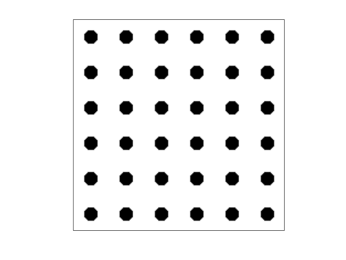
4.2.2 Subspace dimensions
The dimensions of the subspaces and are determined indirectly by the parameters and . A good choice of (and ) is one that returns (and ), and at the same time includes the “important” eigenvectors to enhance convergence to an optimum. In our numerical experiments, we choose which in turn leads to the resulting subspace dimensions and in the range of . Moreover, we find that choosing larger values of and (e.g., ), which in turn increases and and hence increases computational cost, does not yield fewer iterations than choosing .
4.3 Computational Cost
With all the programs implemented in MATLAB and the computation performed on a Linux PC with Dual Core AMD Opteron 270, GHz, a successful run of the algorithm can typically be done in – minutes including – outer iterations, i.e., passes of Steps 2-5 of the main algorithm in Table 1. An example of the computational cost and outer iterations for different band gap optimization is shown in Table 2 as a general illustration of our computational experience.
We point out that these numbers merely represent one set of possibilities; variations in the numerical results are likely to occur with different random initial configurations. Nevertheless, the computation cost does serve as an indication of the general level of difficulty of finding a solution in each problem. In general, lower eigenvalue band gap optimization problems are easier to solve (at least to local optima). Moreover, the table illustrates that TM problems usually solve faster and require fewer outer iterations. This latter observation is consistent with the result reported in [15], and is possibly due to the high non-convexity of the original TE optimization problem.
| Execution time (min) | ||||||||||
|---|---|---|---|---|---|---|---|---|---|---|
| Outer Iterations | ||||||||||
| Execution time (min) | ||||||||||
| Outer Iterations |
Before ending this section, we point out some possible ways to improve the computational cost of our procedure. For the eigenvalue calculation, it is probably helpful to apply a more efficient eigensolver (we used MATLAB’s eigs function in the current implementation). Another promising approach is to explore mesh adaptivity and incorporate non-uniform meshing for the representation of the dielectric function, as well as the eigenvalue calculation. As further discussed in Section 5, it should be possible to significantly reduce the number of decision variables and computation cost with this approach.
4.4 Optimal Structures
We start the optimization procedure with a random distribution of the dielectric, such as the one shown in Figure 5(a). The corresponding band structures of the TE and TM fields are shown in Figure 5(b). In Figure 6, we present an example of the evolution of the crystal structure as the optimization process progresses. (The light color indicates the low dielectric constant and the dark color denotes the high dielectric constant.) As illustrated in Figure 7, the gap-midgap ratio starts from a negative value () corresponding to the random configuration (Figure 7(a)) and increases up to corresponding to the optimal configuration (Figure 7(f)) at which time the optimization process terminates successfully. Another example of the optimization evolution for TE polarization is shown in Figure 8 and Figure 9, in which the gap-midgap ratio increases from to .


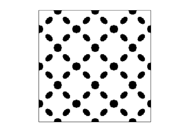
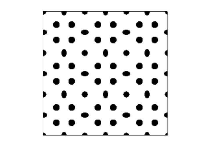
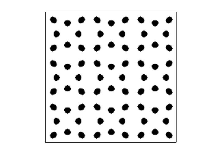
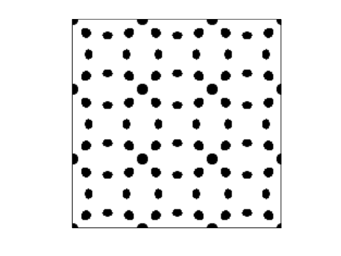
In Figures 10 through 19, we present only plots of the final optimized crystal structures and the corresponding band structures for the through optimized band gaps for TE and TM polarizations. We see that the optimized TM band gaps are exhibited in isolated high- structures, while the optimized TE band gaps appear in connected high- structures. This observation has also been pointed out in [13] (p) “the TM band gaps are favored in a lattice of isolated high- regions, and TE band gaps are favored in a connected lattice”, and observed in [15] previously. For both TE and TM polarizations, the crystal structures become more and more complicated as we progress to higher bands. It would be very difficult to create such structures using physical intuition alone. The largest gap-midgap ratio for the TM case is between the seventh and eighth frequency bands, while the largest ratio for the TE case is , also between the seventh and eighth bands. The results presented here are not guaranteed to be globally optimal, as pointed out in Section 4.2.1. While most crystal structures in the TM cases appear similar to those presented in [15], we have shown quite different TE structures. A qualitative comparison between the two results in the background indicates larger band gaps (both in absolute value and in the gap-midgap ratio) in our results.


5 Conclusions and Future Work
We have introduced a novel approach, based on reduced eigenspaces and semidefinite programming, for the optimization of band gaps of two-dimensional photonic crystals on square lattices. Our numerical results convincingly show that the proposed method is very effective in producing a variety of structures with large band gaps at various frequency levels in the spectrum.
Since our computational techniques make essential use of the finite element method, we anticipate that notions of mesh adaptivity can be easily incorporated into our approach, and thus its computational efficiency will be improved even further. For example, one can start with a relatively coarse mesh and converge to a near-optimal solution, and then judiciously refine the finite element mesh (e.g., refining elements at the interface of dielectric materials) using the current optimal solution at the coarser mesh as the new initial configuration. We intend to explore this approach and report the details and results in a forthcoming paper.
The main strengths of our proposed approach to solve eigenvalue gap optimization problem is the fact that SDP-based methods do not require explicit computation of (sub-)gradients of the objective function (which are ill-defined in the case of eigenvalue multiplicities), hence maintaining the regularity of the formulation. The approach proposed in this paper can also be readily extended to deal with more general problems, such as the optimization of photonic crystals in combined TE and TM fields, optimizing multiple band gaps, dealing with other types of lattices (e.g. triangular), as well as modeling and optimizing the design of three-dimensional photonic crystals.
Acknowledgments. We are grateful to Professor Steven Johnson of the Mathematics Department of MIT for numerous discussions on this research. We thank Professor Lim Kian Meng of National University of Singapore for advising and supporting of H. Men.
References
- [1] F. Alizadeh. Interior point methods in semidefinite programming with applications to combinatorial optimization. SIAM Journal on Optimization, 5(1):13–51, 1995.
- [2] F. Alizadeh, J. P. A. Haeberly, and M. L. Overton. Primal-dual interior-point methods for semidefinite programming: convergence rates, stability and numerical results. SIAM Journal on Optimization, 8(3):746–768, 1998.
- [3] F. Bloch. Über die quantenmechanik der elektronen in kristallgittern. Zeitschrift für Physik A Hadrons and Nuclei, 52(7):555–600, 1929.
- [4] M. Burger, S. J. Osher, and E. Yablonovitch. Inverse problem techniques for the design of photonic crystals. IEICE Trans. Electron. E, 87:258–265.
- [5] E. Cances, C. LeBris, N. C. Nguyen, Y. Maday, A. T. Patera, and G. S. H. Pau. Feasibility and competitiveness of a reduced basis approach for rapid electronic structure calculations in quantum chemistry. In Proceedings of the Workshop for High-dimensional Partial Differential Equations in Science and Engineering (Montreal), volume 41, pages 15–57, 2007.
- [6] A. Charnes and W. W. Cooper. Programming with linear functionals. Naval Research Logistics Quarterly, 9, 1962.
- [7] S. J. Cox and D. C. Dobson. Band structure optimization of two-dimensional photonic crystals in H-polarization. Journal of Computational Physics, 158(2):214–224, 2000.
- [8] B. D. Craven and B. Mond. The dual of a fractional linear program. Journal of Mathematical Analysis and Applications, 42(3):507–512, 1973.
- [9] M. Doosje, B. J. Hoenders, and J. Knoester. Photonic bandgap optimization in inverted fcc photonic crystals. Journal of the Optical Society of America B, 17(4):600–606, 2000.
- [10] S. Fan, J. D. Joannopoulos, J. N. Winn, A. Devenyi, J. C. Chen, and R. D. Meade. Guided and defect modes in periodic dielectric waveguides. Journal of the Optical Society of America B, 12(7):1267–1272, 1995.
- [11] S. Fan, P. Villeneuve, J. Joannopoulos, and H. Haus. Channel drop filters in photonic crystals. Optics Express, 3(1):4–11, 1998.
- [12] G. Floquet. Sur les equations differentielles lineaires a coefficients periodiques. Ann. Ecole Norm. Ser, 2(12):47–89, 1883.
- [13] J. D. Joannopoulos, S. G. Johnson, J. N. Winn, and R. D. Meade. Photonic crystals: molding the flow of light. Princeton university press, 2008.
- [14] S. John. Strong localization of photons in certain disordered dielectric superlattices. Physical Review Letters, 58(23):2486–2489, 1987.
- [15] C. Y. Kao, S. Osher, and E. Yablonovitch. Maximizing band gaps in two-dimensional photonic crystals by using level set methods. Applied Physics B: Lasers and Optics, 81(2):235–244, 2005.
- [16] Y. Nesterov and A. Nemirovskii. Interior-point polynomial algorithms in convex programming. SIAM studies in applied mathematics, 13, 1994.
- [17] G. S. H. Pau. Reduced-basis method for band structure calculations. Physical Review E (Statistical, Nonlinear, and Soft Matter Physics), 76(4):046704, 2007.
- [18] L. Rayleigh. On the maintenance of vibrations by forces of double frequency, and on the propagation of waves through a medium endowed with a periodic structure. Phil. Mag, 24(147):145–159, 1887.
- [19] O. Sigmund and J. S. Jensen. Systematic design of phononic band-gap materials and structures by topology optimization. Philosophical Transactions: Mathematical, Physical and Engineering Sciences, pages 1001–1019, 2003.
- [20] M. Soljacic, S. G. Johnson, M. Ibanescu, Y. Fink, and J. D. Joannopoulos. Optimal bistable switching in nonlinear photonic crystals. Physical Review E, 66:055601, 2002.
- [21] R. H. Tütüncü, K. C. Toh, and M. J. Todd. Solving semidefinite-quadratic-linear programs using SDPT3. Mathematical Programming, 95(2):189–217, 2003.
- [22] L. Vandenberghe and S. Boyd. Semidefinite programming. SIAM review, 38(1):49–95, 1996.
- [23] H. Weyl. Symmetry. Princeton Univ. Press, 1952.
- [24] H. Wolkowicz, R. Saigal, and L. Vandenberghe. Handbook of semidefinite programming: theory, algorithms, and applications. Kluwer Academic Publishers, 2000.
- [25] E. Yablonovitch. Inhibited spontaneous emission in solid-state physics and electronics. Physical Review Letters, 58(20):2059–2062, 1987.
- [26] X. L. Yang, L. Z. Cai, Y. R. Wang, C. S. Feng, G. Y. Dong, X. X. Shen, X. F. Meng, and Y. Hu. Optimization of band gap of photonic crystals fabricated by holographic lithography. EPL-Europhysics Letters, 81(1):14001–14001, 2008.
- [27] M. F. Yanik and S. Fan. Stopping and storing light coherently. Phys. Rev. A, 71(1):013803, Jan 2005.