The Structure of a Low-Metallicity Giant Molecular Cloud ComplexNote: Accepted for publication in The Astrophysical Journal

For consistency among the 70, 100, and 160 $\mu$m data, we move flux densities at 70 and 160 $\mu$m from the MIPS scale (which assumes $F_{\nu}\propto\nu^{2}$ across the bandpass) to the IRAS scale (which assumes $F_{\rm\nu}\propto\nu^{-1}$). We do so by dividing the $70$ map by $0.918$ and the $160\mu$m map by $0.959$.

We subtract Milky Way foreground emission from the 100 and 160$\mu$m maps. We estimate this from Galactic H I assuming the average cirrus dust properties measured by [20]. At 100$\mu$m we use their fit directly; at 160$\mu$m we interpolate their fits assuming a typical cirrus dust temperature ($T=17.5$ K) and emissivity ($\beta=2$).

To refine the foreground subtraction, we assume that H I and infrared intensity from the SMC are correlated at a basic level. As the column density of SMC H I approaches 0, we expect the IR intensity of the SMC to also approach 0. Therefore, we adjust the zero point of the IR maps using a fit of IR intensity to $N\left(\mbox{\rm{H~I}}\right)_{\rm SMC}$ where $N(\mbox{\rm{H~I}})_{\rm SMC}<2\times 10^{21}$ cm^-2 (we subtract the fitted $y$-intercept). This leads us to add $0.3$ MJy ster^-1 at 70 $\mu$m, subtract $4.4$ MJy ster^-1 at 160$\mu$m, and subtract $0.5$ MJy ster^-1 from the IRIS 100$\mu$m map. These offsets are a natural consequence of the uncertainty in the reduction and foreground subtraction (which must remove zodiacal light, Milky Way cirrus, and any cosmic infrared background). Deviations from the average cirrus properties are particularly common, being observed near a number of galaxies by Bot et al. [18].

Based on carrying out this exercise in several different ways, we estimate the zero level of our maps to be uncertain by $0.25$ MJy ster^-1 at 70$\mu$m and $1$ MJy ster^-1 at 160$\mu$m. We take these uncertainties into account in our calculations (§III.2). To minimize their impact we only consider lines of sight with intensities well above the background, by which we mean $I_{70}>0.5$ MJy ster^-1 and $I_{160}>2$ MJy ster^-1 after the foreground subtraction (i.e., twice the uncertainty in the background).

In the rest of this paper we will combine the data described above in several ways. Two of these combinations lead to maps combining data with different resolutions. We comment on these here and the reader may wish to refer back to this section while reading the paper.

First, we subtract a foreground component measured at $14\arcmin$ resolution from IR maps with $4.3\arcmin$ and $\sim 36\arcsec$ (160$\mu$m) resolution. Any small scale variation in the Milky Way cirrus will therefore be left in our maps. This is only a concern in the diffuse region of the Wing (and so only in §IV.1). In N83 itself most lines of sight exhibit FIR intensities $\gtrsim 10$ times higher than the foreground, so variations in the foreground are not a concern.

Second, when estimating the distribution of H₂ in N83, we derive the total amount of hydrogen ($\mbox{\rm{H~I}}+\mbox{\rm H${}_{2}$}$) along a line of sight and then subtract the measured H I column density. The total amount of hydrogen is based on FIR dust emission, measured at $36\arcsec$ resolution (or $55\arcsec$ resolution when we compare to the SEST CO $J=1\rightarrow 0$ map). The H I column density is measured at $98\arcsec$ resolution. We assume it to be smooth on smaller scales, an assumption born out to some degree by the reasonable correlation that we find between H₂ and CO. Nonetheless, the detailed distribution of H₂ on scales less than $98\arcsec$ ($\sim 29$ pc) is somewhat uncertain.

In assuming that $I_{\rm 100}/I_{\rm 160}$ traces $T_{\rm dust}$ or its more sophisticated analogs [26, 33, e.g.,], we follow several recent studies of the Magellanic Clouds [16, 59, 8, 42]. Schnee et al. [86], Schnee et al. [84], Schnee et al. [85] have demonstrated that a similar approach reproduces optical and near-IR extinction in Galactic molecular clouds, though with some systematic uncertainties.

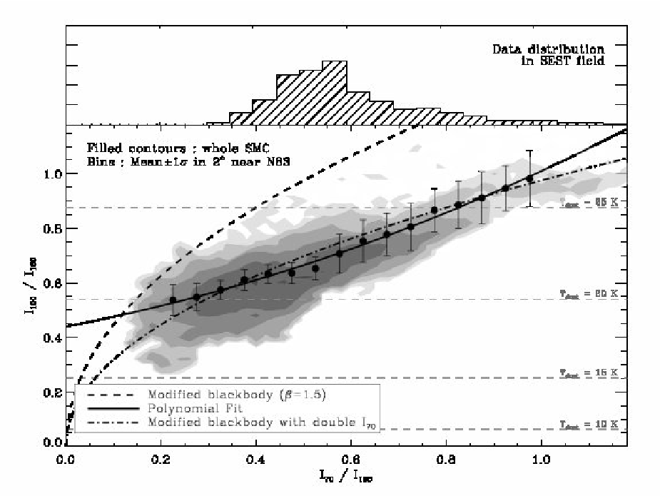
Figure 2 motivates our use of $I_{\rm 70}/I_{\rm 160}$ ($x$-axis) to predict $I_{\rm 100}/I_{\rm 160}$ ($y$-axis). Gray contours show the distribution of data for the whole SMC. Bins (filled circles) show data from a $2\arcdeg$ square field centered on N83 (i.e., Figure 1). Both near N83 and over the whole SMC, the two colors show a reasonable correlation (rank correlation coefficient $0.7$).

Figure 2 also motivates our ad hoc treatment of the conversion between $I_{\rm 70}/I_{\rm 160}$ and $I_{\rm 100}/I_{\rm 160}$. A single modified blackbody (the dashed line shows one with $\beta=1.5$) cannot simultaneously describe the SMC at 70, 100, and 160$\mu$m. The simplest explanation is that $I_{\rm 100}/I_{\rm 160}$ traces $T_{\rm dust}$, while the 70$\mu$m band includes substantial non-equilibrium emission. We tested the possibility of using the models of Draine & Li [33], which include the effects of stochastic heating, to directly derive dust masses from $I_{70}/I_{160}$. However, the currently available “SMC” models cannot reproduce the data in Figure 2. Bot et al. [16] and Bernard et al. [8] showed that a similar case holds for the Desert et al. [28] models. The main stumbling block is reproducing the observed 60$\mu$m [28] or 70$\mu$m [33] emission.

Equation 3 is not a unique description. A simple alternative is a modified blackbody with twice the expected emission at $70\mu$m. In this case:

The aim of this paper is not to investigate the details of small grain heating in the SMC, so we move forward using our empirical fit (Equation 3). This appears as a solid line in Figure 2. It is a good match to the data near N83, where the RMS scatter in the color of individual pixels about the fit is $\approx 0.04$. In deriving uncertainties we use Equation 4 as an equally valid alternative to Equation 3.

To convert from $I_{100}/I_{160}$ to $T_{\rm dust}$ we assume that the SED along each line of sight is described by a modified blackbody with $\tau_{\lambda}\propto\lambda^{-\beta}$. At long wavelengths ($\lambda\gtrsim 100\mu$m), a blackbody spectrum with a wavelength–dependent emissivity is indeed a good description of the integrated SED of the SMC [2, 98, 59]. We take $\beta=1.5$, which is intermediate in the range of plausible values [32, e.g.,] and a reasonable description of the integrated SMC SED from $\lambda\sim 100$–$1000\mu$m. This is not strongly preferred, and so we allow $\beta$ from $1.0$ to $2.0$ in our assessment of uncertainties.

We assess the uncertainty in $\tau_{160}$ by repeatedly adding realistic noise to our 70 and 160$\mu$m data and then deriving $\tau_{160}$ under varying assumptions. For each realization, we offset the observed 70 and 160$\mu$m maps by a random amount to reflect uncertainty in the background subtraction; these offsets are drawn from normal distributions with $1\sigma=0.25$ MJy ster^-1 at 70$\mu$m and 1 MJy ster^-1 at 160$\mu$m. We add normally distributed noise to each map. This noise has amplitude equal to the measured noise (§II) and is correlated on scales of $36\arcsec$.

We derive $I_{\rm 100}/I_{\rm 160}$ for each realization using either the polynomial fit (Equation 3) or scaling the 70$\mu$m intensity (Equation 4), with equal probability of each. We add normally distributed noise to $I_{\rm 100}/I_{\rm 160}$ with $1\sigma=0.04$ (the RMS residual about Equations 3 and 4) and then derive $T_{\rm dust}$ assuming $\beta$ anywhere from 1.0 to 2.0 with equal probability.

This entire process is repeated 1,000 times. We use the distribution of Monte Carlo $\tau_{160}$s for each pixel to estimate a realistic uncertainty, finding individual measurements to be uncertain by $\approx 40\%$ ($1\sigma$). We extend the same approach through our derivation of $N\left(\mbox{\rm H${}_{2}^{\rm FIR}$}\right)$ in §IV.4. In Appendix A we discuss systematic effects that cannot be straightforwardly incorporated into this approach, two of which (blended dust populations and hidden cold dust) could impact $\tau_{\rm 160}$.

It will be useful to make an approximate assessment of the dust column in terms of $V$-band line-of-sight extinction, $A_{V}$, and reddening, $E(B-V)$. In the Solar Neighborhood, $E(B-V)=N\left({\rm H}\right)/5.8\times 10^{21}~{\rm cm}^{-2}$ [10] and $\tau_{160}=2.44\times 10^{-25}~{\rm cm}^{2}~N\left(\mbox{\rm{H~I}}\right)$ [20, studying the Galactic cirrus where we may safely assume that $N({\rm H})\approx N(\mbox{\rm{H~I}})$]. Then

Estimates of $A_{V}$ and $E(B-V)$ based on $\tau_{160}$ and Equations III.3 and 5 agree well with optical- and UV-based measurements. Caplan et al. [25] compiled $A_{V}$ for a number of SMC H II regions, including N83 and N84A/B (both of which lie within the SEST field). Towards N83 they find $A_{V}$ in the range $0.42$–$0.79$ mag (mean $0.63$ mag); towards N84A/B they found $A_{V}$ from $0.24$–$0.60$ mag (mean $0.37$ mag). Using their positions and aperture sizes, we derive $A_{V}=1.34\pm 0.36$ mag and $0.93\pm 0.26$ mag for the same regions. The optical and UV measurements are based on absorption toward sources inside the SMC. Therefore they will sample half the total line-of-sight extinction on average. Accounting for this, our FIR-based extinction estimates are in excellent agreement with optical values. We find the same good agreement for Sk 159, a B star near N83 towards which Fitzpatrick [38] and Tumlinson et al. [94] measured $E(B-V)\approx 0.05$ mag, while we estimate $E(B-V)=0.08\pm 0.03$ mag (see §IV.3).

In Figure 3, we plot $\tau_{160}$ as a function of $N(\mbox{\rm{H~I}})$ over the $2\arcdeg$ field centered on N83. Most of the data are well-described by

Equation 8 is consistent within the uncertainties with results of Bot et al. [16], who found $\tau_{\rm 160}\sim\left(1.0\pm 0.5\right)\times 10^{-26}~{\rm cm}^{2}~N(\mbox{\rm{H~I}})~\left[{\rm cm^{-2}}\right]$ for the whole Wing (after adjusting for slight differences in $T_{\rm dust}$, $\beta$, and $\lambda$). In the Solar Neighborhood, $\tau_{160}\approx 2.44\times 10^{-25}~{\rm cm}^{2}~N(\mbox{\rm{H~I}})~\left[{\rm cm^{-2}}\right]$ [20]. Comparing this to Equation 8 implies that the $DGR$ near N83 is $17^{+10}_{-6}$ times smaller than the Galactic value. This agrees within the uncertainties with the $DGR$ found for the SMC Wing by Leroy et al. [59], which is $\approx 10^{+10}_{-5}$ lower than Galactic¹¹ 1 Leroy et al. [59] made no correction for H I opacity. Doing so would improve the agreement with the present measurement..

From Equations 8 and III.3, we estimate $N({\rm H})/E(B-V)\approx 10^{+6}_{-4}\times 10^{22}$ cm^-2 mag^-1. This matches the SMC–average $N({\rm H})/E(B-V)\approx 8.7\times 10^{22}$ cm^-2 mag^-1 measured by Fitzpatrick [39] using IUE and confirmed by Tumlinson et al. [94] with FUSE.

Equation 8 and Figure 3 demonstrate that a single $DGR$ describes the region near N83 well. The notable exceptions are a small number of points with high $\tau_{\rm 160}$ relative to their H I column density. In Figure 4 we show the distribution of residuals about Equation 8. Contours indicate where our Monte Carlo uncertainty estimates yield 85, 98, and 99.9% confidence that the residuals are really greater than zero.

The neighboring panel shows the same confidence contours superimposed on an H$\alpha$ image of the region near N83 (Winkler et al., private communication). The highest residuals are associated with N83 itself. Other regions with higher-than-expected $\tau_{\rm 160}$ are also associated with concentrations of H$\alpha$ emission. H$\alpha$ emission indicates ongoing massive star formation, which in turn suggests the presence of H₂. N83 also has significant CO emission, another signpost of H₂ [69]. If a large amount of the ISM is H₂, we expect high residuals about Equation 8 even for a fixed $DGR$.

To derive H${}_{2}^{\rm FIR}$ from Equation 6 over the SEST field, we must know the $DGR$ in N83 itself. We cannot measure this directly because we do not have an independent measure of the H₂ column. We might expect $DGR$ in N83 to differ somewhat from that in the surrounding diffuse gas of the Wing: stars are more likely to form in regions with high $DGR$ and the denser environment may shelter grains from destruction by shocks or lead to grain growth [36, e.g.,]. In addition to our measurement of the diffuse ISM, we consider two pieces of evidence when adopting a $DGR$ to use in N83: observations of a nearby B star and the metallicity of the N84C H II region.

FUSE and IUE Measurements of Sk 159: From FUSE and IUE absorption measurements, $E(B-V)$, $N(\mbox{\rm H${}_{2}$})$, and $N(\mbox{\rm{H~I}})$ are known towards Sk 159, a B0.5 star near N83 (marked by a star in Figure 4). H₂ is detected but the column density is small [3, $\approx 2\times 10^{19}$ cm^-2,]. The reddening associated with the SMC is $\approx 0.05$ mag [38, 94], though somewhat uncertain. The H I column measured from absorption along the same line of sight is $2\pm 1\times 10^{21}$ cm^-2 [19], roughly half of the column inferred from 21 cm emission along the line of sight (two kinematically distinct H I components are visible in emission towards Sk 159; only one of them is seen in absorption, implying that Sk 159 sits between the two, behind the smaller one). These values imply $N({\rm H})/E(B-V)\approx 2$–$6\times 10^{22}$ cm^-2 mag^-1, or $DGR\approx 2$–$7\times 10^{-26}$ cm².

Metallicity of N84C: Russell & Dopita [83] measured the nebular metallicity of the N84C H II region, which lies within the SEST field, finding $12+\log{\rm O/H}=8.27$, $2$–$3$ times lower than the Solar Neighborhood value and among the highest for any region the SMC. Translating metallicity into a $DGR$ is not totally straightforward, because the fraction of heavy elements tied up in dust may vary with environment. For a fixed fraction of heavy elements in dust, one would expect $DGR\propto Z^{-1}$. Fits to samples of galaxies yield power law relationships ($DGR\propto Z^{\alpha}$) with indices in the range $\alpha=1$–$2$ [61, 31, e.g.,]. This would imply $N({\rm H})/E(B-V)\sim 2$–$7\times 10^{22}$ cm^-2 mag^-1 or $DGR\sim 2$–$7\times 10^{-26}$ cm².

H I and $\tau_{160}$: Equation 8 offers a lower bound on the $DGR$ — N83 is extremely unlikely to have a lower $DGR$ than the surrounding medium ($N({\rm H})/E(B-V)\approx 10\times 10^{22}$ cm^-2 mag^-1) and from absorption work we know that there is not a pervasive massive molecular component in the SMC. The magnitude of the residuals about this equation towards N83 itself also offer a weak upper bound on the quantity. If we assume $DGR$ much above $3$ times the value in Equation 8 then some lines of sight inside the SEST field will have significantly negative residuals. If the star-forming region itself is described by a single $DGR$, then it must be roughly bounded by this value, which translates to $N({\rm H})/E(B-V)\sim 3\times 10^{22}$ cm^-2 mag^-1.

Assumed $DGR$ in N83: The relatively high metallicity and the measurement towards Sk 159 are balanced against our observations of a very low $DGR$ in the nearby ISM and the requirement that $\Sigma_{\rm H2}^{\rm FIR}$ not be significantly and systematically negative. The former suggest $N({\rm H})/E(B-V)\sim 2$–$7\times 10^{22}$ cm^-2 mag^-1, while the latter yields $N({\rm H})/E(B-V)\sim 3$–$10\times 10^{22}$ cm^-2 mag^-1. In the remainder of this paper we adopt assume that in N83 itself $N({\rm H})/E(B-V)\sim 5\times 10^{22}$ cm^-2 mag^-1, which is intermediate in this range. Then

Combining Equations 6 and 9 we estimate $N(\mbox{\rm H${}_{2}^{\rm FIR}$})$ from $\tau_{160}$ and $N(\mbox{\rm{H~I}})$. From $N(\mbox{\rm H${}_{2}^{\rm FIR}$})$, we calculate the molecular gas surface density,

The right column in Figure 5 shows the resulting maps of $\Sigma_{\rm H2}^{\rm FIR}$ in N83 at the resolution of the SEST CO $2\rightarrow 1$ (top) and $1\rightarrow 0$ (bottom) data. The left column shows the CO maps. Note that the stretch on the H${}_{2}^{\rm FIR}$ images runs linearly from $\Sigma_{\rm H2}^{\rm FIR}=100$ M_⊙ pc^-2 to $500$ M_⊙ pc^-2.

Several systematic uncertainties may affect $N\left(\mbox{\rm H${}_{2}^{\rm FIR}$}\right)$ but are hard to quantify and so not reflected in our Monte Carlo estimate of the uncertainties. We consider these in Appendix A, finding no strong reason to doubt that Equation 6 yields an approximate estimate of $N(\mbox{\rm H${}_{2}$})$.

Before we consider the relationship between CO, H${}_{2}^{\rm FIR}$, and dust within N83, we briefly examine the transition from atomic (H I) to molecular (H₂) gas in the complex.

Krumholz et al. [54] recently considered the transition from H I to H₂ in galaxies. They argue that inside a complex of mixed atomic and molecular gas, the ratio of H₂ to H I along a line of sight ($R_{\rm H2}=\Sigma_{\rm H2}/\Sigma_{\rm HI}$) is mainly a function of two factors: total gas surface density ($\Sigma_{\rm HI}+\Sigma_{\rm H2}$) and metallicity. Their calculations agree well with a variety of observations, including FIR-based estimates of $\Sigma_{\rm H2}$ in the SMC at lower resolution.

Comparing H I and H₂ in the area around N83, we indeed observe a clear relationship between $R_{\rm H2}$ and the total gas surface density. We show this in Figure 6, plotting $R_{\rm H2}$ against $\Sigma_{\rm HI}+\Sigma_{\rm H2}^{\rm FIR}$ over the whole area where $\Sigma_{\rm H2}^{\rm FIR}>0$. We work at the $98\arcsec$ (29 pc) resolution of the H I map, with each point in the plot showing an independent measurement. For this analysis, we are interested in the gas associated with the star-forming complex itself (not unassociated gas in front of and behind it along the line of sight). To remove H I unassociated with N83 itself from $\Sigma_{\rm HI}$, we subtract the median $\Sigma_{\rm HI}$ measured over the area shown in Figure 1 ($53$ M_⊙ pc^-2) from the measured $\Sigma_{\rm HI}$ before plotting. This is only an issue for H I; H${}_{2}^{\rm FIR}$ does not extend beyond the N83 complex.

We overplot the relationship between $R_{\rm H2}$ and $\Sigma_{\rm HI}+\Sigma_{\rm H2}$ predicted by Krumholz et al. [54] for three metallicities: $Z=0.5$, $0.33$, and $0.125$ times solar. Our data are consistent with the shape of the Krumholz et al. [54] calculation. We find $R_{\rm H2}=1$ at $\Sigma_{\rm H2}+\Sigma_{\rm HI}=68\pm 12$ M_⊙ pc^-2, which agrees well with their calculations for $Z$ 2-3 times lower than the solar value. This is roughly the metallicity measured for the N84C H II region [83]. However, it is significantly higher than the $DGR$ that we adopt (§IV.3), which is closer to the lower value. Because Krumholz et al. [54] assume a linear scaling between dust opacity and metallicity when deriving these curves, this means that there remains some disagreement between our measurements and their results. Nonetheless, there is good qualitative agreement in the shape of the curve and the fact that in N83 $R_{\rm H2}=1$ at a significantly higher value of $\Sigma_{\rm HI}+\Sigma_{\rm H2}$ than in a solar metallicity cloud.

Figure 5 shows that the distributions of H${}_{2}^{\rm FIR}$ and CO share the same peaks and basic morphology. However, the values of $I_{\rm CO}$ in N83 are low compared to a Galactic molecular cloud, which usually show $I_{\rm CO}\sim 10$ K km s${}^{{}_{1}}$ over a large area, not merely the peaks [99, e.g.,]. By contrast, the values of $\Sigma_{\rm H2}^{\rm FIR}$ (mean $180$ M_⊙ pc^-2) are similar to the surface density of an average Galactic GMC $\sim 120$–$170$ M_⊙ pc^-2 [87, 45].

This means that CO is faint compared to H${}_{2}^{\rm FIR}$ in N83. Over the SEST field $X_{\rm CO}$ is

The left panel in Figure 7 compares H${}_{2}^{\rm FIR}$ and $I_{\rm CO}$ for individual lines of sight. We plot $\Sigma_{\rm H2}^{\rm FIR}$ as a function of $I_{\rm CO}$ over the SEST field. We regrid the data so that each point corresponds to an approximately independent measurement over a $\sim 10$ pc (CO $J=2\rightarrow 1$) or $\sim 17$ pc (CO $J=1\rightarrow 0$) wide box. Gray curves show fixed CO-to-H₂ conversion factors, starting with Galactic (lowest) and increasing by factors of 3.33.

As with Figure 5, Figure 7 shows that despite the very low ratio of CO to H${}_{2}^{\rm FIR}$, the two exhibit an overall correspondence. High $I_{\rm CO}$ coincides with high $\Sigma_{\rm H2}^{\rm FIR}$ and the reverse, so that a rank correlation coefficient of $0.7$ relates the two over the SEST field.

The relationship between $I_{\rm CO}$ and $\Sigma_{\rm H2}^{\rm FIR}$ does not go through the origin. Instead, $I_{\rm CO}=0$ corresponds to roughly $\Sigma_{\rm H2}^{\rm FIR}=50$–$150$ M_⊙ pc^-2. This suggests the presence of an envelope of H${}_{2}^{\rm FIR}$ with very little or no associated CO. Unfortunately, this result is very sensitive to the adopted $DGR$ (§IV.3 and Appendix A). If we take $DGR$ at the upper end of the plausible range, the data are consistent with no CO-free envelope although CO emission is still faint relative to $\Sigma_{\rm H2}^{\rm FIR}$ in the SEST field. If we take $DGR$ at the value derived in the nearby diffuse ISM, the surface density of the envelope is even higher $\sim 200$-$400$ M_⊙ pc^-2. Although the observation towards Sk 159 does not actually intersect the envelope in the latter case, it is very nearby and the low $N(\mbox{\rm H${}_{2}$})$ derived from absorption towards this star offers some circumstantial evidence against a very massive extended envelope.

The other notable feature of this plot is that at very high $\Sigma_{\rm H2}^{\rm FIR}$ CO intensity increases dramatically (the turn to the right at the top of the plot). We see this in both CO transitions, but the effect is more pronounced at the higher resolution of the CO $J=2\rightarrow 1$ data, suggesting that the bright CO-emitting structures are still relatively small compared to the SEST beam. The result is that the line-of-sight integrated ratio of H${}_{2}^{\rm FIR}$ to CO is lower for the regions of brightest CO emission, dropping to $\sim 15$ times the Galactic value. Care must be taken interpreting these ratios because H${}_{2}^{\rm FIR}$ and CO emission almost certainly trace different volumes (§V.4).

In §I, we highlighted the role of dust in shielding CO from dissociating radiation. This may provide a simple explanation for the upturn in CO intensity at high $\Sigma_{\rm H2}^{\rm FIR}$. Lequeux et al. [58] modeled CO emission in SMC molecular clouds. For their typical cloud ($n_{\rm H}\sim 10^{4}$ cm^-3, illuminated by a radiation field 10 times the local interstellar radiation field), they found that most CO emission comes from a relatively narrow region of the cloud centered on $A_{V}\sim 1$ mag. Outside this regime CO intensity is very weak, a scenario that qualitatively matches what we see in the left panel of Figure 7 [6, see also].

In the right panel of Figure 7 we plot CO intensity as a function of line-of-sight extinction, $A_{V}$. We estimate $A_{V}$ from $\tau_{160}$ using Equation 5. For comparison, we mark $A_{V}\sim 2$ mag, the line-of-sight extinction that roughly matches the depth from which Lequeux et al. [58] predict most CO emission to emerge (see their Figures 2 and 6). They model a slab illuminated from one side while we estimate the total extinction along the line of sight through the cloud. Therefore $A_{V}=1$ mag for them corresponds to $A_{V}\sim 2$ mag for us (though the actual geometry is likely to be much more complicated). We also plot the relationship between extinction and CO intensity measured in the Pipe Nebula (a nearby Milky Way cloud) by Lombardi et al. [62, see their Figure 22]. We convert $A_{K}$ into $A_{V}$ using their adopted $A_{V}=A_{K}/0.112$. They measure a scatter of roughly $2$ K km s^-1 about this relation.

In agreement with Lequeux et al. [58], we find that lines of sight with bright CO emission occur almost exclusively above $A_{V}\sim 2$ mag. Our maps lack the dynamic range in $A_{V}$ to test whether $I_{\rm CO}$ is indeed more or less independent of extinction well above this threshold [62, 75, as in the Milky Way,]. In fact, Figure 3a of Lequeux et al. [58] seems a close match to what we observe: a shallow slope that steepens sharply around $A_{V}$ of 2 mag (for us). The radiation field that they assume, $10$ times the Galactic value is a rough match to what one would infer comparing $T_{\rm dust}$ in N83 (median $\sim 23$ K, max $\sim 28$ K) to that of Galactic cirrus (17.5 K) — median $\sim 5$, maximum $\sim 15$³³ 3 For our adopted $\beta=1.5$, the magnitude of the radiation field heating the dust is roughly $\propto T^{5.5}$. — especially when one recalls that this is integrated over the whole line of sight rather than tracing the radiation field incident on the cloud surface.

N83 shows somewhat less CO at a given extinction than the Pipe Nebula. This is also in agreement with the models by Lequeux et al. [58], which predict that CO from Milky Way clouds emerges from a broader range of $A_{V}$ and lower values of $A_{V}$ than in the SMC. They attribute the difference to lower rates of photodissociation and it certainly seems likely that the radiation field incident on the H₂ in N83 is much more intense than in the relatively quiescent Pipe.

Small differences should not overshadow the similarities between the CO-extinction relation in the Milky Way and that in the SMC. Compared to the left panel in Figure 7, the right panel actually shows a striking similarity between Galactic and SMC clouds. We derive a CO-H₂ conversion that differs with the Milky Way by a factor of $\sim 30$, while the relationship between extinction and CO is only slightly offset. Figure 7 supports the hypothesis that shielding, rather than the distribution of H₂, determines the location of bright CO emission. Here “shielding” refers to a combination of dust and self-shielding. Both processes are important to setting the location at which most C is tied up in CO [102, e.g.,] and the effective shielding from both sources will be weaker in the SMC than in the Galaxy due to the decreased metallicity.

Extinction may also be critical to a cloud’s ability to form stars. McKee [66] proposed that ionization by an external radiation field plays an important role in setting cloud structure because it determines the degree of magnetic support. He predicted that clouds forming low-mass stars in equilibrium will self-regulate to achieve integrated line-of-sight extinctions $A_{V}\approx 4$–$8$ mag. These extinctions are higher than the $A_{V}\sim 2$–$3$ mag that we find towards the CO peaks N83 or the average extinction over the region, $A_{V}\sim 1.5$ mag. We can safely conclude that the N83 region as a whole does not resemble the equilibrium low-mass star forming cloud described by McKee [66]. If these equilibrium structures do exist in this region, they must be compact relative to our $10$ pc beam. Bolatto et al. [13] find that the dynamics of CO emission in the SMC also appear to disagree with the predictions of McKee [66] but present several important caveats to the comparison. The most important of these here is that McKee [66] explicitly consider clouds forming only low-mass stars, while N83 is quite obviously actively producing high mass stars.

We emphasize that this comparison between CO and $A_{V}$ is fairly robust. It does not depend on our choice of $DGR$, only on the adopted FIR emissivity ($\tau_{\rm FIR}/A_{V}$) and reddening law. The most likely biases in the emissivity (e.g., coagulation of small grains) will lower $A_{V}$, bringing our results into even closer agreement with those in the Milky Way.

CO line emission also offers kinematic information. This is the basis of the virial mass method commonly used to estimate the masses of molecular clouds and derive CO-to-H₂ conversion factors [81, 100, 5, e.g.], including in N83 [12, 52, 13]. The potential pitfall of this approach may be seen from §V.3: if CO emission is confined to regions with extinction above a certain threshold and these regions represent only a fraction of the whole cloud, then velocity dispersion and size measured from CO observations will only be lower than their true values. Mass outside the region of CO emission may exert pressure on the surface of the “CO cloud,” but it is not straightforward to estimate the total mass of a cloud from observing kinematics from only part of it. As a result, in a low-metallicity cloud like N83, we expect virial masses from CO observations to be smaller than H${}_{2}^{\rm FIR}$ (even over matched areas) because the latter also traces the outer (CO-free) part of the cloud, which exists in front of and behind the CO-emitting region even over matched lines of sight.

In N83, we have the advantage of an independent measurement of H${}_{2}^{\rm FIR}$ and observing the CO emission over a range of scales. Here we test whether these observations can be reconciled using a simple model in which CO emission comes from only the inner part of a larger H₂ cloud (as appears to be the case in N83). We consider a spherical cloud with a radially declining density, such that $\rho\propto r^{-\alpha}$, and a radius $R$ beyond which $\rho=0$, i.e., the model usually adopted (with $\alpha=1$) to calculate cloud virial masses [87]⁴⁴ 4 We cap the density at its maximum value over the inner $3\%$ of the cloud to avoid divergence.. We assume that the dynamical mass estimated from CO line data traces the mass of a fraction of this cloud, out to radius $r_{\rm frac}$. The ratio of dynamical mass to H${}_{2}^{\rm FIR}$ over a matched area, $M_{\rm vir}/M_{\rm H2}^{\rm FIR}$ is then a function of $\alpha$ and the ratio of the true radius of the cloud to the radius of the area being considered, $r_{\rm frac}/R$. The top left panel of Figure 8 shows this ratio for models with $\alpha$ from 0 to 2.0.

To compare our observations to this model, we measure the line width and radius of CO emission over a series of scales in N83. We consider intensity contours in position-position-velocity space, beginning with the bright northwestern region and including progressively more of the cloud (but always including that region, see Figure 8). We estimate the radius and line width of each region from the area (for the radius) and second moment (for the line width). To account for the finite resolution of SEST, the radius of each cloud is adjusted by

For each contour, we measure $M_{\rm vir}/M_{\rm H2}^{\rm FIR}$. We compare this ratio as a function of $R$ to a range of density profiles and cloud radii. The resulting distribution of reduced $\chi^{2}$ is shown in the bottom left panel of Figure 8. Our measurements, along with the best-fit model are shown in the bottom right panel of the same figure.

The best-fit model has $\rho\propto r^{-0.6}$ and $R=70$ pc, though these numbers are not strongly constrained. The $\chi^{2}=1$ surface spans $R=50$ – $140$ pc and $\alpha=0.2$ – $0.8$. Moreover, the assumption of a virial parameter equal to 1 (i.e., that Equation 13 holds) is questionable both because we neglect support by magnetic fields, non-circular geometries, and surface pressure terms (while considering substructure inside of a larger cloud). Even more generally, the fundamental assumption that clouds or parts of clouds are virialized is not certain to hold.

Despite these concerns, Figure 8 does demonstrate that a simple model — CO emission nested inside a larger sphere of H₂— can relate dynamics measured from molecular line emission and H${}_{2}^{\rm FIR}$. The best fit radius, $R=70$ pc, is quite similar to that needed to achieve the extinction threshold for CO emission ($A_{V}\approx 1$) using our adopted $DGR$ and $n\approx 100$ cm^-3 — a typical average volume density for Galactic GMCs and perhaps appropriate for the diffuse gas between dense molecular clumps in the SMC. These three numbers combine to yield a depth of $\sim 60$ pc. Meanwhile, the density profile is similar to the $\alpha=1$ commonly used to describe Galactic clouds [87].

The strong dependence of $M_{\rm vir}/M_{\rm H2}^{\rm FIR}$ on the size-scale sampled at least partially motivates the discrepancy between CO-to-H₂ conversion factors measured using CO observations and those derived from dust. At the high resolutions achieved by millimeter-wave interferometers in Local Group galaxies, CO-emitting clouds are resolved from their surroundings. By concentrating on these clouds, one samples only dense regions where CO is well-shielded by dust. This naturally leads to relatively modest conversion factors. On the other hand, dust measurements and dynamical measurements made on larger scales sample the whole complex. In the SMC this appears to includes a large amount of poorly-shielded gas and such methods therefore return significantly larger conversion factors. One manifestation of this phenomenon is that dynamical mass determinations from CO measurements with larger physical beam sizes often return systematically and significantly higher conversion factors than those obtained from CO measurements in much smaller beams [82, 100, 46, 12]. For interferometer measurements to properly sample the full cloud structure a multi-scale analysis, such as that presented here or the more rigorous “dendogram” approach recently described by Rosolowsky et al. [78], is necessary.

Although our dynamical and dust-based results appear consistent with this simple picture, other recent results suggest a more complex relationship between the two measurements. Bot et al. (2009, in prep.) recently measured the relationship between sub-millimeter dust emission and CO-based dynamical masses in the southwest part of the SMC Bar. Even after controlling for contamination by an extended superstructure of CO-free H₂, they find that virial masses are systematically lower than dust-based H₂ masses on the scale of individual CO-bright regions. This might arise if clouds are short-lived (i.e., presently collapsing) or partially supported by magnetic fields. Alternatively it may reflect altered dust properties in dense cloud cores. The virial-dust discrepancy measured by Bot et al. and the multiscale virial-dust measurements presented here can both be readily applied to simulated clouds and multi-tracer observations of Galactic GMCs. It will be interesting to see whether these measurements can be replicated purely by altering the CO-emitting surface inside of a cloud (as it appears from our simple model) or if they constrain SMC cloud structure to be genuinely different from that in the Milky Way (as appears to be the case from the Bot et al. results).

References

- [1] Abergel, A., Boulanger, F., Mizuno, A., & Fukui, Y. 1994, ApJ, 423, L59
- [2] Aguirre, J. E., Bezaire, J. J., Cheng, E. S., Cottingham, D. A., Cordone, S. S., Crawford, T. M., Fixsen, D. J., Knox, L., Meyer, S. S., Norgaard-Nielsen, H. U., Silverberg, R. F., Timbie, P., & Wilson, G. W. 2003, ApJ, 596, 273
- [3] André, M. K., Le Petit, F., Sonnentrucker, P., Ferlet, R., Roueff, E., Civeit, T., Désert, J.-. M., Lacour, S., & Vidal-Madjar, A. 2004, A&A, 422, 483
- [4] Arce, H. G., & Goodman, A. A. 1999, ApJ, 512, L135
- [5] Arimoto, N., Sofue, Y., & Tsujimoto, T. 1996, PASJ, 48, 275
- [6] Bell, T. A., Roueff, E., Viti, S., & Williams, D. A. 2006, MNRAS, 371, 1865
- [7] Bernard, J. P., Abergel, A., Ristorcelli, I., Pajot, F., Torre, J. P., Boulanger, F., Giard, M., Lagache, G., Serra, G., Lamarre, J. M., Puget, J. L., Lepeintre, F., & Cambrésy, L. 1999, A&A, 347, 640
- [8] Bernard, J.-P., Reach, W. T., Paradis, D., Meixner, M., Paladini, R., Kawamura, A., Onishi, T., Vijh, U., Gordon, K., Indebetouw, R., Hora, J. L., Whitney, B., Blum, R., Meade, M., Babler, B., Churchwell, E. B., Engelbracht, C. W., For, B.-Q., Misselt, K., Leitherer, C., Cohen, M., Boulanger, F., Frogel, J. A., Fukui, Y., Gallagher, J., Gorjian, V., Harris, J., Kelly, D., Latter, W. B., Madden, S., Markwick-Kemper, C., Mizuno, A., Mizuno, N., Mould, J., Nota, A., Oey, M. S., Olsen, K., Panagia, N., Perez-Gonzalez, P., Shibai, H., Sato, S., Smith, L., Staveley-Smith, L., Tielens, A. G. G. M., Ueta, T., Van Dyk, S., Volk, K., Werner, M., & Zaritsky, D. 2008, AJ, 136, 919
- [9] Blitz, L., Fukui, Y., Kawamura, A., Leroy, A., Mizuno, N., & Rosolowsky, E. 2007, in Protostars and Planets V, ed. B. Reipurth, D. Jewitt, & K. Keil, 81–96
- [10] Bohlin, R. C., Savage, B. D., & Drake, J. F. 1978, ApJ, 224, 132
- [11] Bolatto, A. D., Jackson, J. M., & Ingalls, J. G. 1999, ApJ, 513, 275
- [12] Bolatto, A. D., Leroy, A., Israel, F. P., & Jackson, J. M. 2003, ApJ, 595, 167
- [13] Bolatto, A. D., Leroy, A. K., Rosolowsky, E., Walter, F., & Blitz, L. 2008, ApJ, 686, 948
- [14] Bolatto, A. D., Simon, J. D., Stanimirović, S., van Loon, J. T., Shah, R. Y., Venn, K., Leroy, A. K., Sandstrom, K., Jackson, J. M., Israel, F. P., Li, A., Staveley-Smith, L., Bot, C., Boulanger, F., & Rubio, M. 2007, ApJ, 655, 212
- [15] Boselli, A., Lequeux, J., & Gavazzi, G. 2002, A&A, 384, 33
- [16] Bot, C., Boulanger, F., Lagache, G., Cambrésy, L., & Egret, D. 2004, A&A, 423, 567
- [17] Bot, C., Boulanger, F., Rubio, M., & Rantakyro, F. 2007, A&A, 471, 103
- [18] Bot, C., Helou, G., Boulanger, F., Lagache, G., Miville-Deschenes, M.-A., Draine, B., & Martin, P. 2009, ArXiv e-prints
- [19] Bouchet, P., Lequeux, J., Maurice, E., Prevot, L., & Prevot-Burnichon, M. L. 1985, A&A, 149, 330
- [20] Boulanger, F., Abergel, A., Bernard, J.-P., Burton, W. B., Desert, F.-X., Hartmann, D., Lagache, G., & Puget, J.-L. 1996, A&A, 312, 256
- [21] Boulanger, F., Bronfman, L., Dame, T. M., & Thaddeus, P. 1998, A&A, 332, 273
- [22] Brüns, C., Kerp, J., Staveley-Smith, L., Mebold, U., Putman, M. E., Haynes, R. F., Kalberla, P. M. W., Muller, E., & Filipovic, M. D. 2005, A&A, 432, 45
- [23] Cambrésy, L., Boulanger, F., Lagache, G., & Stepnik, B. 2001, A&A, 375, 999
- [24] Cambrésy, L., Jarrett, T. H., & Beichman, C. A. 2005, A&A, 435, 131
- [25] Caplan, J., Ye, T., Deharveng, L., Turtle, A. J., & Kennicutt, R. C. 1996, A&A, 307, 403
- [26] Dale, D. A., & Helou, G. 2002, ApJ, 576, 159
- [27] Dame, T. M., Hartmann, D., & Thaddeus, P. 2001, ApJ, 547, 792
- [28] Desert, F.-X., Boulanger, F., & Puget, J. L. 1990, A&A, 237, 215
- [29] Dickey, J. M., Mebold, U., Marx, M., Amy, S., Haynes, R. F., & Wilson, W. 1994, A&A, 289, 357
- [30] Dickey, J. M., Mebold, U., Stanimirović, S., & Staveley-Smith, L. 2000, ApJ, 536, 756
- [31] Draine, B. T., Dale, D. A., Bendo, G., Gordon, K. D., Smith, J. D. T., Armus, L., Engelbracht, C. W., Helou, G., Kennicutt, Jr., R. C., Li, A., Roussel, H., Walter, F., Calzetti, D., Moustakas, J., Murphy, E. J., Rieke, G. H., Bot, C., Hollenbach, D. J., Sheth, K., & Teplitz, H. I. 2007, ApJ, 663, 866
- [32] Draine, B. T., & Lee, H. M. 1984, ApJ, 285, 89
- [33] Draine, B. T., & Li, A. 2007, ApJ, 657, 810
- [34] Dutra, C. M., Ahumada, A. V., Clariá, J. J., Bica, E., & Barbuy, B. 2003, A&A, 408, 287
- [35] Dwek, E. 1997, ApJ, 484, 779
- [36] —. 1998, ApJ, 501, 643
- [37] Elmegreen, B. G. 1989, ApJ, 338, 178
- [38] Fitzpatrick, E. L. 1984, ApJ, 282, 436
- [39] —. 1985, ApJS, 59, 77
- [40] Fukui, Y., Mizuno, N., Yamaguchi, R., Mizuno, A., Onishi, T., Ogawa, H., Yonekura, Y., Kawamura, A., Tachihara, K., Xiao, K., Yamaguchi, N., Hara, A., Hayakawa, T., Kato, S., Abe, R., Saito, H., Mano, S., Matsunaga, K., Mine, Y., Moriguchi, Y., Aoyama, H., Asayama, S.-i., Yoshikawa, N., & Rubio, M. 1999, PASJ, 51, 745
- [41] Galliano, F., Madden, S. C., Jones, A. P., Wilson, C. D., Bernard, J.-P., & Le Peintre, F. 2003, A&A, 407, 159
- [42] Gordon, K. D., Bot, C., Muller, E., Misselt, K. A., Bolatto, A., Bernard, J. ., Reach, W., Engelbracht, C. W., Babler, B., Bracker, S., Block, M., Clayton, G. C., Hora, J., Indebetouw, R., Israel, F. P., Li, A., Madden, S., Meade, M., Meixner, M., Sewilo, M., Shiao, B., Smith, L. J., van Loon, J. T., & Whitney, B. A. 2008a, ArXiv e-prints
- [43] Gordon, K. D., Clayton, G. C., Misselt, K. A., Landolt, A. U., & Wolff, M. J. 2003, ApJ, 594, 279
- [44] Gordon, K. D., Engelbracht, C. W., Rieke, G. H., Misselt, K. A., Smith, J.-D. T., & Kennicutt, Jr., R. C. 2008b, ApJ, 682, 336
- [45] Heyer, M., Krawczyk, C., Duval, J., & Jackson, J. M. 2008, ArXiv e-prints
- [46] Israel, F. 2000, in Molecular Hydrogen in Space, ed. F. Combes & G. Pineau Des Forets, 293–+
- [47] Israel, F. P. 1988, in Astrophysics and Space Science Library, Vol. 147, Millimetre and Submillimetre Astronomy, ed. R. D. Wolstencroft & W. B. Burton, 281–305
- [48] Israel, F. P. 1997a, A&A, 317, 65
- [49] —. 1997b, A&A, 328, 471
- [50] Israel, F. P., de Graauw, T., van de Stadt, H., & de Vries, C. P. 1986, ApJ, 303, 186
- [51] Israel, F. P., Johansson, L. E. B., Lequeux, J., Booth, R. S., Nyman, L. A., Crane, P., Rubio, M., de Graauw, T., Kutner, M. L., Gredel, R., Boulanger, F., Garay, G., & Westerlund, B. 1993, A&A, 276, 25
- [52] Israel, F. P., Johansson, L. E. B., Rubio, M., Garay, G., de Graauw, T., Booth, R. S., Boulanger, F., Kutner, M. L., Lequeux, J., & Nyman, L.-A. 2003, A&A, 406, 817
- [53] Issa, M. R., MacLaren, I., & Wolfendale, A. W. 1990, A&A, 236, 237
- [54] Krumholz, M. R., McKee, C. F., & Tumlinson, J. 2009, ApJ, 693, 216
- [55] Larson, R. B. 1981, MNRAS, 194, 809
- [56] Laureijs, R. J., Clark, F. O., & Prusti, T. 1991, ApJ, 372, 185
- [57] Lee, H., Skillman, E. D., Cannon, J. M., Jackson, D. C., Gehrz, R. D., Polomski, E. F., & Woodward, C. E. 2006, ApJ, 647, 970
- [58] Lequeux, J., Le Bourlot, J., Des Forets, G. P., Roueff, E., Boulanger, F., & Rubio, M. 1994, A&A, 292, 371
- [59] Leroy, A., Bolatto, A., Stanimirović, S., Mizuno, N., Israel, F., & Bot, C. 2007, ApJ, 658, 1027
- [60] Leroy, A., Bolatto, A., Walter, F., & Blitz, L. 2006, ApJ, 643, 825
- [61] Lisenfeld, U., & Ferrara, A. 1998, ApJ, 496, 145
- [62] Lombardi, M., Alves, J., & Lada, C. J. 2006, A&A, 454, 781
- [63] Madden, S. C., Galliano, F., Jones, A. P., & Sauvage, M. 2006, A&A, 446, 877
- [64] Madden, S. C., Poglitsch, A., Geis, N., Stacey, G. J., & Townes, C. H. 1997, ApJ, 483, 200
- [65] Maloney, P., & Black, J. H. 1988, ApJ, 325, 389
- [66] McKee, C. F. 1989, ApJ, 345, 782
- [67] Meixner, M., Gordon, K. D., Indebetouw, R., Hora, J. L., Whitney, B., Blum, R., Reach, W., Bernard, J.-P., Meade, M., Babler, B., Engelbracht, C. W., For, B.-Q., Misselt, K., Vijh, U., Leitherer, C., Cohen, M., Churchwell, E. B., Boulanger, F., Frogel, J. A., Fukui, Y., Gallagher, J., Gorjian, V., Harris, J., Kelly, D., Kawamura, A., Kim, S., Latter, W. B., Madden, S., Markwick-Kemper, C., Mizuno, A., Mizuno, N., Mould, J., Nota, A., Oey, M. S., Olsen, K., Onishi, T., Paladini, R., Panagia, N., Perez-Gonzalez, P., Shibai, H., Sato, S., Smith, L., Staveley-Smith, L., Tielens, A. G. G. M., Ueta, T., Dyk, S. V., Volk, K., Werner, M., & Zaritsky, D. 2006, AJ, 132, 2268
- [68] Miville-Deschênes, M.-A., & Lagache, G. 2005, ApJS, 157, 302
- [69] Mizuno, N., Rubio, M., Mizuno, A., Yamaguchi, R., Onishi, T., & Fukui, Y. 2001, PASJ, 53, L45
- [70] Ossenkopf, V., & Henning, T. 1994, A&A, 291, 943
- [71] Ott, J., Wong, T., Pineda, J. L., Hughes, A., Muller, E., Li, Z.-Y., Wang, M., Staveley-Smith, L., Fukui, Y., Weiß, A., Henkel, C., & Klein, U. 2008, Publications of the Astronomical Society of Australia, 25, 129
- [72] Pak, S., Jaffe, D. T., van Dishoeck, E. F., Johansson, L. E. B., & Booth, R. S. 1998, ApJ, 498, 735
- [73] Papadopoulos, P. P., Thi, W.-F., & Viti, S. 2002, ApJ, 579, 270
- [74] Pelupessy, F. I., Papadopoulos, P. P., & van der Werf, P. 2006, ApJ, 645, 1024
- [75] Pineda, J. E., Caselli, P., & Goodman, A. A. 2008, ApJ, 679, 481
- [76] Rosolowsky, E., Engargiola, G., Plambeck, R., & Blitz, L. 2003, ApJ, 599, 258
- [77] Rosolowsky, E., & Leroy, A. 2006, PASP, 118, 590
- [78] Rosolowsky, E. W., Pineda, J. E., Kauffmann, J., & Goodman, A. A. 2008, ApJ, 679, 1338
- [79] Rubio, M., Boulanger, F., Rantakyro, F., & Contursi, A. 2004, A&A, 425, L1
- [80] Rubio, M., Garay, G., Montani, J., & Thaddeus, P. 1991, ApJ, 368, 173
- [81] Rubio, M., Lequeux, J., & Boulanger, F. 1993a, A&A, 271, 9
- [82] Rubio, M., Lequeux, J., Boulanger, F., Booth, R. S., Garay, G., de Graauw, T., Israel, F. P., Johansson, L. E. B., Kutner, M. L., & Nyman, L. A. 1993b, A&A, 271, 1
- [83] Russell, S. C., & Dopita, M. A. 1990, ApJS, 74, 93
- [84] Schnee, S., Bethell, T., & Goodman, A. 2006, ApJ, 640, L47
- [85] Schnee, S., Li, J., Goodman, A. A., & Sargent, A. I. 2008, ApJ, 684, 1228
- [86] Schnee, S. L., Ridge, N. A., Goodman, A. A., & Li, J. G. 2005, ApJ, 634, 442
- [87] Solomon, P. M., Rivolo, A. R., Barrett, J., & Yahil, A. 1987, ApJ, 319, 730
- [88] Stanimirovic, S., Staveley-Smith, L., Dickey, J. M., Sault, R. J., & Snowden, S. L. 1999, MNRAS, 302, 417
- [89] Stepnik, B., Abergel, A., Bernard, J.-P., Boulanger, F., Cambrésy, L., Giard, M., Jones, A. P., Lagache, G., Lamarre, J.-M., Meny, C., Pajot, F., Le Peintre, F., Ristorcelli, I., Serra, G., & Torre, J.-P. 2003, A&A, 398, 551
- [90] Strong, A. W., & Mattox, J. R. 1996, A&A, 308, L21
- [91] Thronson, Jr., H. A. 1988, in NATO ASIC Proc. 232: Galactic and Extragalactic Star Formation, ed. R. E. Pudritz & M. Fich, 621–+
- [92] Thronson, Jr., H. A., Greenhouse, M., Hunter, D. A., Telesco, C. M., & Harper, D. A. 1988, ApJ, 334, 605
- [93] Thronson, Jr., H. A., Walker, C. K., Walker, C. E., & Maloney, P. 1987, ApJ, 318, 645
- [94] Tumlinson, J., Shull, J. M., Rachford, B. L., Browning, M. K., Snow, T. P., Fullerton, A. W., Jenkins, E. B., Savage, B. D., Crowther, P. A., Moos, H. W., Sembach, K. R., Sonneborn, G., & York, D. G. 2002, ApJ, 566, 857
- [95] Walter, F., Cannon, J. M., Roussel, H., Bendo, G. J., Calzetti, D., Dale, D. A., Draine, B. T., Helou, G., Kennicutt, Jr., R. C., Moustakas, J., Rieke, G. H., Armus, L., Engelbracht, C. W., Gordon, K., Hollenbach, D. J., Lee, J., Li, A., Meyer, M. J., Murphy, E. J., Regan, M. W., Smith, J.-D. T., Brinks, E., de Blok, W. J. G., Bigiel, F., & Thornley, M. D. 2007, ApJ, 661, 102
- [96] Walter, F., Taylor, C. L., Hüttemeister, S., Scoville, N., & McIntyre, V. 2001, AJ, 121, 727
- [97] Walter, F., Weiss, A., Martin, C., & Scoville, N. 2002, AJ, 123, 225
- [98] Wilke, K., Klaas, U., Lemke, D., Mattila, K., Stickel, M., & Haas, M. 2004, A&A, 414, 69
- [99] Wilson, B. A., Dame, T. M., Masheder, M. R. W., & Thaddeus, P. 2005, A&A, 430, 523
- [100] Wilson, C. D. 1995, ApJ, 448, L97+
- [101] Wilson, C. D., Scoville, N., Madore, B. F., Sanders, D. B., & Freedman, W. L. 1988, ApJ, 333, 611
- [102] Wolfire, M. G., Hollenbach, D., & Tielens, A. G. G. M. 1993, ApJ, 402, 195
Appendix A Systematic Uncertainties in
Several systematic uncertainties may affect but are hard to quantify and so not reflected in our Monte Carlo estimate of the uncertainties. Here we discuss these for the specific case of N83 [48, for a more general discussion see]. We find no strong reason to doubt that Equation 6 yields an approximate estimate of . N83 appears unlikely to harbor a significant population of cold dust and we do not observe compelling evidence that dust traces mostly warm ionized gas or high optical depth H I. There is likely some blending of populations along the line of sight, but the magnitude of the effect is unclear. Grain processing is largely unconstrained, but we note the dissimilarity between N83 and the dense, cold cores where these effects are usually discussed.
Blending of Populations Along the Line of Sight: N83 is a dense, active region and the line-of-sight distance through the SMC may be very long. As a result, the observed dust emission may represent a blend of several dust populations with different temperatures. The likely effect is that we overestimate the average along the line of sight and therefore underestimate and H [84, e.g., see tests on simulated clouds by].
Cold Dust: A related concern is that our longest wavelength data are at m. As a result, we would miss any population of cold dust. In the Milky Way, when cold, molecular filaments can be isolated from embedded star formation, they are often observed to have low dust temperatures ( K) and little out-of-equilibrium emission [56, 7, 89, e.g.,]. As with blending of several populations, cold dust is most likely to be associated with the dense, molecular environment of N83. Missing cold dust would lead us to underestimate and .
Given the high in N83 and the presence of ongoing, vigorous star formation we consider it unlikely that there is a significant amount of cold dust present. We attempt a simple test that reveals the presence of cold filaments in Galactic GMCs [1, 21]: we take the median over the region, scale the m map by this value, and subtract it from the 160m map. This should reveal the location of any local 160m excess, a likely signature of cold dust. We find no such excess associated with N83 as a whole or the CO peaks in particular.
Other Gas Phases: We refer to the results of Equation 6 as ”H” but this is actually an estimate of all gas not traced by the 21-cm transition. Some of this might be high optical depth H I or warm ionized gas. Neither appears to be a plausible explanation for the majority of such gas in N83. This agrees with results from the Milky Way, where excess dust emission identified in a similar way also appears to correspond mostly to H2[27].
The right panel in Figure 9 shows the H I opacities required to account for in N83 given our adopted . These values, –, are higher than those implied by the fit of Dickey et al. [30], which yields a maximum line-integrated (correction factor ) near N83. Indeed, most of the line-integrated values of in Figure 9 are higher than any of the peak values (i.e., in the most opaque velocity channel) measured by Dickey et al. [30] in the SMC (maximum ). though that study did not probe any star-forming peaks; toward the starburst region 30 Doradus in the LMC Dickey et al. [29] found peak values of , which is still too small to achieve the line-integrated value of required account for in N83. The 21cm spectra do show some evidence of optical thickness at a brightness temperature of K, but no clear signs of self-absorption at the velocity of the CO peak (left panel in Figure 9). We cannot rule out unlucky geometry, but achieving line-integrated optical depths of – without invoking a contrived scenario appears difficult.
Warm ionized gas also seems unlikely to account for most of H. The left panel in Figure 10 shows contours of over an H image (at matched resolution) in the SEST field. Although high residuals correspond to H emission on large scales, the detailed distribution is not a particularly good match. The rank correlation coefficient between H and H over the area observed by SEST is , much lower than the relating H and CO. H emission is proportional to and so obviously a flawed tracer of the true warm gas column (), but the poor correspondence on small scales still argues that most H is not actually warm ionized gas.
Dust Processing in Molecular Clouds: A significant but hard-to-constrain uncertainty in Equation 6 is if and how dust properties vary between N83 and the surrounding ISM. The most likely variations are increases in the FIR emissivity or the . In the Milky Way, the FIR emissivity of dust () does appear to increase towards dense regions, increasing by – above mag [4, 34, 24, e.g.,]. Cambrésy et al. [23], Stepnik et al. [89], and Cambrésy et al. [24] argue that this is due to the creation of fluffy dust grains with low albedos [35] via grain-grain coagulation or accretion of gas. At the same time, build-up of existing grains in molecular clouds and dust creation in Type II supernovae or stellar winds [36, e.g.,] may cause the ratio near star-forming regions to be higher than in the surrounding ISM.
The magnitude of grain growth in GMCs remains very poorly constrained and in an active environment like N83 it will be balanced against grain destruction (e.g., in shocks). Further, the high dust temperatures, low integrated extinctions ( mag almost everywhere), and weak CO emission in N83 are a far cry from the high density, high extinction environments in which grain coagulation or the formation of icy mantles are usually modeled or observed [70, e.g.,]. Moreover, as pointed out by Bernard et al. [8], increased emissivity in Milky Way clouds is often associated with diminished small grain emission [85, e.g.,], while N83 exhibits increased compared to its surroundings.
Because it is unclear what, if any, grain processing is at work in N83, we make no correction to the emissivity. If dust in N83 indeed has a high emissivity compared to the diffuse ISM, we will derive values of both and that are too high. Note that our adopted is already twice that in the surrounding diffuse gas. Increasing or decreasing the adopted will not affect or , but will lower or raise .
Effect of Changing on the CO-H2 relation: The exact value of the in N83 is the largest systematic uncertainty in our analysis. We discuss the constraints on this quantity in §IV.3. In the right panel of Figure 10, we illustrate the relationship between H2 and in the limiting cases: equal to that in the diffuse ISM of the SMC Wing (black) and equal to three times this value (gray).
There are two main conclusions to draw from this comparison. First, the existence and magnitude of a truly CO-free H2 envelope (the -intercept of the points) depends sensitively on the adopted ; the lowest plausible value is (partially by construction) consistent with no envelope and the highest value implies an envelope with surface densities – M⊙ pc-2, – times the average surface density of a Galactic GMC. Second, the average CO-to-H2 conversion factor varies between and times Galactic over the full range of possible . The qualitative behavior (meaning the presence of bright only above a certain threshold) remains the same. We emphasize that the relationship between (or ) and is unaffected by the choice of .