Model Independent Constraints Among the , , and Couplings
Abstract
Using an effective Lagrangian approach, we perform a model-independent analysis of the interactions among electroweak gauge bosons and the third generation quarks, i.e. the , and couplings. After one imposes the known experimental constraint on the coupling, we show that the electroweak symmetry of the standard model specifies the pattern of deviations of the and couplings, independent of underlying new physics scenarios. We study implications of the predicted pattern with data on the single top quark and associated production processes at the Large Hadron Collider. Such an analysis could in principle allow for a determination of the coupling without prior knowledge of , which is otherwise difficult to achieve.
I Introduction
It is widely accepted that interactions of the third generation quarks, the top and bottom quarks, offer a window into possible new physics beyond the standard model (SM) of particle physics. Since the top quark mass is close to the Fermi scale , its interactions are thought to be sensitive to the mechanism of electroweak symmetry breaking. Indeed, in the majority of models beyond the SM, deviations are predicted from the SM in the top quark interactions, especially in their couplings with the electroweak gauge bosons, such as the , , and couplings. Interactions of the top quark have yet to be measured precisely, allowing possible room for deviations from the SM. Experimental constraints on the bottom and top quark couplings with the and bosons provide an interesting contrast: the bottom quark left-handed coupling is determined precisely by the measurements at LEP I and II [1], whereas the coupling is virtually not measured so far. The coupling was confirmed only recently in single top quark production at the Fermilab Tevatron [2, 3, 4]. It will be probed further at the CERN Large Hadron Collider (LHC).
In this work we investigate the range of possible deviations of the couplings of the top and bottom quarks with the electroweak gauge bosons by exploiting the contrasting experimental constraints mentioned above. Adopting an effective Lagrangian approach [5], we parametrize the effects of new physics in terms of higher dimensional operators constructed from SM fields: , where is the mass dimension of the operator , is the scale of new physics, and is a numerical coefficient assumed to be of order unity unless otherwise specified. Such an approach is valid when all new particles are heavier than the Fermi scale and whose effects can be integrated out of the effective theory, as we assume. However, this assumption does not preclude the possibility that new particles at the TeV scale could be produced directly and observed at the LHC.
Within the general context in which we work, we demonstrate that the symmetry of the SM yields correlations among the possible deviations of the couplings , , and . Once the stringent experimental bound on is taken into account, a unique prediction follows on the size of the and couplings. The prediction is a striking manifestation of invariance, and it is independent of the underlying new physics at the electroweak scale.
After an exposition of the general operator analysis in Section II, we use existing experimental constraints to show that deviations of the and couplings from their SM values can depend on only two parameters, and , and we present the allowed ranges of these parameters for different new physics cutoff scales and Higgs boson masses. In Section III, we survey the landscape of new physics models which may be expected to modify these couplings. The prospects that and can be determined better from data from the LHC are addressed in Section IV where we focus on single top quark and associated production. Our results from Section II show deviations from the SM of the single top quark total and differential cross sections depend only on , whereas the cross section for associated production is influenced by both and .
The presence of contributions from two operators in associated production means that observation, or at least a bound on the effects of new physics in this process is in principle possible provided one looks sufficiently differentially into the distributions of particles in the final state. We began our study expecting to show that spin correlations in the final state would offer significant advantages, particularly those between the top quark spin and the decay lepton from . However, as we conclude from a detailed simulation in Sec. IV, experimental cuts distort the most telling distributions and appear to leave a sample of effectively unpolarized top quarks. This result, while disappointing, does not appear to have been established previously. Turning adversity to advantage, we remark that the difficulty in finding evidence for new physics in the final state may be interpreted as good news for new physics searches. The associated production of is a dominant background for new physics models [6, 7]. If a new physics model predicts the production of highly polarized top quark pairs, then one might be able to see evidence above the effectively unpolarized dominant background. Among the final state distributions in associated production, we confirm that the opening angle between the two charged leptons from the boson decay, , appears useful for limiting the couplings and , as is pointed out in Ref. [8].
We also comment that in single top quark production is always multiplied by the CKM matrix element , which is very close to one in the SM. Therefore if both and could be extracted from production through the total and differential cross-sections, one could infer the value of from measurements in singlet top quark production.
We present the results of our analysis as a set of two-dimensional plots of the deviation from the SM of the associated production cross section versus the deviation of the single top quark cross section for integrated luminosities of and at the LHC. These expectations are contrasted with estimates for a high energy electron-positron linear collider (LC). A comparison is also shown with predictions based on recent models of new physics including a top-prime model [9], a right-handed model [10], and a model with sequential fourth generation quarks that mix with the third generation [11]. Our analysis suggests that about at the LHC would be needed to improve model independent constraints on and to the same level achievable at a 500 GeV LC with of integrated luminosity. On the other hand, at the LHC would be sufficient to delineate which new physics models could be possible.
In addition to the study in Ref. [8] of associated production mentioned above, other earlier work related to ours includes the study in Ref. [12] of the prospects for measuring the coupling at a linear collider as a test of different models of new physics. The authors investigate production and single top quark production, as we do, but they do not focus on the correlations.
II Operator Analysis and Existing Constraints
We begin with a general assumption that effects beyond the SM are described by a set of higher dimensional operators made out of the SM fields only. Once the (approximate) symmetry of the SM is assumed, these operators start at dimension six [5]. A complete list of operators is presented in [13], whose notation we follow. Therefore the effective Lagrangian we work with is of the form
| (1) |
where the coefficients ’s are numerical constants parameterizing the strength of the non-standard interactions. The excellent agreement between the SM expectations and data indicates that deviations from the SM are small. Hence, when computing the effects of new operators we can restrict ourselves to the interference terms between and the operators , i.e. we can work to first order in the coefficients .
II.1 Operator Analysis
Three types of dimension-six operators contribute to the , , and couplings: 1) operators involving scalars and vectors, 2) operators involving fermions and vectors, and 3) operators involving vectors, fermions, and scalars. We discuss all three types in turn in the following.
Operators involving scalars and vectors enter through the self-energy of the electroweak gauge boson: , , and , where denotes the SM scalar Higgs doublet, and are the field-strength tensors for the and gauge bosons respectively, and is the usual generator in the fundamental representation. Operators and arise only after new physics is integrated out at the loop level [14]. Their corrections to the self-energy are of order , where is the vacuum expectation value of the Higgs. Operator can be generated by tree-level exchange of new particles, but its contribution is related to the parameter. It is highly constrained by precision electroweak data, which requires [15] for TeV. Thus, all three operators are effectively suppressed by a loop factor for new physics at about the 1 TeV scale, and we neglect them in this study.
Operators of the second type necessarily have two fermions carrying one gauge-covariant derivative and one field strength [13], such as . These operators give a correction of order to the couplings of interest here, where is the typical momentum scale in the process and can be taken to be the Fermi scale . However, such operators correspond to vertices with only three legs. They appear only once new physics is integrated out at the loop level [14, 16, 17]. Their natural size is again of order . A similar conclusion can be obtained from naive dimensional analysis [18], since each derivative in the operator carries an extra suppression. Therefore, we do not consider operators of the second type here.
Operators of the third type can be generated both at the tree-level and at the loop level. The loop-induced operators, such as , , , and , are not included in our analysis as they are suppressed by small coefficients of order [14]. We focus our attention on the tree-level induced operators of the third type throughout this paper.
The dimension-six operators of the third type are
| (2) | |||||
| (3) | |||||
| (4) | |||||
| (5) | |||||
| (6) |
where is the gauge-covariant derivative; is the left-handed top-bottom doublet ; are the corresponding right-handed isosinglets; and is the two-dimensional antisymmetric tensor. Corrections from these operators are of order and could be generated from integrating out new physics at the tree-level. For example, the operator can be induced by a heavy quark mixing with the top quark, which is present in many theories beyond the SM.
It is worth mentioning that equations of motion can be used to turn the operator into type 3) operators that are universal in flavors [19]. Thus, the statement we are about to make applies to contributions from as well.
Upon symmetry breaking . The set of operators of the third type generate the following corrections to the couplings , and :
| (7) | |||||
| (8) | |||||
| (9) |
where and are the coupling strengths of the and gauge interaction, respectively.
II.2 Existing Constraints
Among the five operators listed above, is tightly constrained by recent data on the rare decay of , [20, 21, 22, 23], provided there is no accidental cancellation with contributions from other new physics effects, such as those produced by the four-fermion operator . 11 1 This operator can be generated, for example, by exchanging a heavy vector boson. As a result, effects from are small and are not considered further.
For the purpose of our analysis, the most useful experimental constraints on the five operators of the third type are the precise measurements of and at LEP II [1]. These bound the coupling. The measured value of the coupling agrees with the SM prediction at the 0.25% level. It enforces the relation
| (10) |
which, in turn, implies that the deviations in the and couplings are controlled by the same parameter . In other words, the symmetry of the SM predicts a certain pattern in the deviations of the electroweak gauge boson couplings to the third generation quarks that is independent of the possible new physics beyond the SM.
Certain subgroups of the custodial symmetry [24] which protect the parameter can also preserve the coupling in the SM [25], resulting in exactly. This result is obtained if the top and bottom quarks are embedded in suitable representations of whose diagonal group serves as the custodial symmetry. If one implements the custodial symmetry in this way, the coupling is also protected, [25]. In this work we are not concerned with the underlying reason for the smallness in the deviation in the coupling. We take Eq. (10) as an empirical statement, allowing us to be model-independent. A recent study of top compositeness and the third generation couplings to electroweak gauge bosons within the the framework of Ref. [25] can be found in Ref. [26].
After Eq. (10) is imposed, the and couplings depend on only two unknown parameters:
| (11) | |||||
| (12) |
where , , and is the cosine of the Weinberg angle. Notice the relation between the coefficients of the left-handed neutral and charged currents 22 2 A similar relation is pointed out in Ref. [27] in the context of an electroweak chiral Lagrangian, even though the implication of such a relation was not studied.:
| (13) |
This equation states the pattern of deviations predicted by the electroweak symmetry of the SM, after the stringent constraint on is imposed. Notice further that the right-handed coupling does not enter the stated correlation in the and couplings, leaving room for the interesting possibility that could be (partially) composite. As it turns out, a positive shift of the coupling, say , would explain the deviation in the forward-backward asymmetry measured by the LEP and SLAC Large Detector experiments [28].
Within the low-energy effective theory, and in induce one-loop corrections to the parameter and the vertex, which are associated with the observables and summarized in Ref. [29]. The pure SM one-loop contributions to and are [30]
| (14) | |||||
| (15) |
where denotes the mass of Higgs boson (-boson, -boson, top quark), respectively. The contributions from the anomalous couplings and are [21]
| (16) | |||||
| (17) |
where is the cutoff of the low-energy effective theory and is taken to be the scale of new physics. Notice that depends on , which implies that the allowed region of and will depend on as well as on .


Using the experimental results [29],
we plot the experimental constraints on and in Fig. 1, assuming the absence of contributions from other operators. It is important to contrast the allowed region for and with the expected sizes based on the power counting discussed earlier in Section II.1. As expected, the constraints from one-loop corrections do not require the magnitudes of and to be smaller than their natural sizes, see Fig. 1(d-f).
Last, we comment on other new physics effects which could modify the above bounds. It is worth mentioning that many tree-level induced operators can also contribute to decay, diluting the constraints we derived above without breaking the correlations between the , and effective couplings. For example, four-fermion operators would affect decay via seagull type loop diagrams. An exploration of the constraints (or correlations) among all tree-level induced operators from the parameter and LEP data is highly desirable, but it is beyond the scope of this paper and will be presented elsewhere. Therefore, we take the above constraints as an indication of the magnitude of the effective couplings but do not limit ourselves to the above parameter space in the subsequent collider analysis.
III New Physics Scenarios
Having established in a model independent fashion the possible pattern of deviations in the , , and couplings, we offer a brief survey in this section of new physics models that give rise to such deviations. The treatment here is by no means complete and serves only to exemplify the generality of the operator analysis.
As discussed in the previous section, we are interested mainly in deviations arising from non-oblique corrections, which are much less constrained experimentally. The simplest possibilities for such corrections are new particles mixing with the SM top quark, the SM bottom quark, or both.
The possibility of introducing additional bottom-like quarks (), which mix with the SM quark, to resolve the discrepancy of the forward-backward asymmetry of the quark () is investigated in Ref. [31]. However, because of the stringent constraint on , the mixing could be significant only in the right-handed sector, implying negligible deviations in the coupling. Since the coupling is already severely constrained by data, as mentioned previously, we do not expect this class of models to produce significant deviations in the and couplings.
A custodial symmetry would protect simultaneously the parameter and the coupling [25]. In this case significant mixing of with the SM quark in the left-handed sector is possible, provided additional top-like quarks with appropriate quantum numbers are also present so as to cancel the contribution to . Explicit examples are found in Refs. [32, 33, 34].
The third class of models we discuss has an exotic top-like () quark which could mix with the SM top quark. Such a scenario appears quite often in theories beyond the SM, especially those attempting to address the quantum stability of the Higgs boson mass. As is well-known, within the SM the largest contribution to the one-loop quadratic divergence of the Higgs boson mass comes from the top quark. Therefore, if the Higgs boson mass is to be at the order of a few hundred GeV without significant fine-tuning, a new particle (i.e., the quark) must be present to cancel the top quark contribution in the quadratic divergence. This is the case in models where the Higgs boson arises as a pseudo-Nambu-Goldstone boson such as in Little Higgs theories [35], the holographic Higgs model [36], the twin Higgs model [37], and so forth. On the other hand, there are also models with a quark which may not deal with the electroweak hierarchy problem explicitly. Notable examples are those with flat [38] or warped [39] extra dimensions where the SM field propagate. In this case the quark is nothing but the Kaluza-Klein partner of the SM top quark, taken to be the zero mode. Very recently a quark was also invoked to explain a possible experimental excess at the Tevatron [9].
Having surveyed some candidates for new physics beyond the SM, to which our model independent analysis applies, we address in the next section how to constrain the two unknown parameters and at the LHC.
IV Measurements of the and couplings at the LHC
In this section we discuss how the and couplings could be measured at the LHC. The former can be measured most directly in single top quark production and the latter in the associated production. We first consider extracting and from total cross section measurements. Then we look beyond the total cross section and study differential distributions in the decay products of associated production.
IV.1 Current Experimental Bounds
Single top quark events result from the -channel process (), the -channel process () and associated production (). The distinct kinematics of each of these processes allows differentiation among their contributions. Observation of single top quark production was reported recently by the CDF and D0 collaborations [3, 4]. These results provide the first direct measurement of the product of the coupling () and the CKM matrix element . CDF quotes and a limit at the C.L. [for ]. D0 obtains and a limit of at the C.L. []. The limit on is derived under assumption of , i.e. . However, the bound can also be translated into a bound on if one assumes the unitarity of the CKM matrix element (). Taking the D0 result at face value and inserting , we see that these data could allow , roughly twice the size shown in Fig. 1.
On the other hand, obvious limitations have precluded measurements of the coupling () thus far. There was insufficient center-of-mass energy at LEP to produce a top quark pair via . At hadron colliders, production is so dominated by the QCD processes and that the signal from via cannot be extracted. However, one might be able to measure the coupling via the process of .
The sensitivity to non-standard couplings at the LHC via single top quark production is investigated in several papers [40, 27, 41, 42, 43, 44, 12, 45], while a study on extracting the coupling in associated production at the LHC appears in Refs. [8, 46]. Such measurements would also be a focus of study in a future high energy electron-positron linear collider (LC).
It is worth pointing out that, since measurements of single top quark production can only probe the combination , it would be desirable to measure independently of , which could be achieved by utilizing associated production.
IV.2 Cross sections for single top quark and associated production
Because the operator is proportional to , only the overall normalization of the single top quark cross section is affected, and, except for normalization, the final state differential distributions are insensitive. A measurement of requires a very precise measurement of the total cross section. The coupling also affects top quark decay, but it does not change the top quark decay branching ratio, i.e. .33 3 Whatever contributes to the matrix element of the decay is canceled by its modification to the top quark decay width. On the other hand, the amplitude involves both and , and it is conceivable that differential distributions in the decay products of production would have different sensitivity to and , respectively. We will look at two possibilities: the opening angle from the decay of and the spin correlation between the top quark and the decay products.
The inclusive cross sections for single top quark and associated production at the LHC are:
| (18) | |||||
| (19) |
where and denote the SM cross sections for single top quark production and production, respectively. We include the possibility of a non-unitary CKM matrix element . From Eq. (18) we see immediately the possibility of extracting from
| (20) |
which is not possible from measurements of single top quark production alone. In the above, could in principle be measured from differential distributions in associated production, as is discussed in detail below.
Since new physics contributions to the , , and couplings are of the order for TeV, we can safely ignore interference effects between new physics and SM one-loop contributions in the total cross section. Therefore, the SM quantities in Eq. (18) are understood to be evaluated at one-loop level, as calculated in Refs. [47, 48, 49, 50, 51, 52, 53, 54, 55, 56, 57, 58, 59, 60].


We define the deviation of the cross sections from the SM predictions as The contours of in the plane of and are shown in Fig. 2(a). The ranges of and in this figure are consistent with the allowed regions shown in Fig. 1. All the contours are straight lines since we keep only the interference term. The anticipated deviation is as large as 20%. We observe that in Eq. (19) and contribute with opposite signs, implying partial cancellations in the new physics contributions. In fact, if then , as one may see in the black-solid curve of Fig. 2(a). On the other hand, if we could infer immediately that , and vice versa. The correlation between the deviations of the cross sections for various values of is revealed in Fig. 2(b), where is assumed. When the right-handed coupling is not modified by any new physics, say , then
| (21) |
as illustrated by the black-solid curve in Fig. 2(b). Non-zero values of increase the intercept on the -axis of all the lines in Fig. 2, as is always negative. The solid bands in the figure are the 3 standard deviation statistical variations of the SM total cross section for different luminosities. Given large enough deviations in both and single top quark production, one could determine the values of and uniquely if . (For example, one can determine by substituting derived from the single top quark measurement into the measurement.) If one relaxes the constraint on then the two measurements merely yield a relation between and , see Eq. (20). Nevertheless, it may be possible to extract independently from differential distributions in , as these are sensitive to the anomalous couplings. If one takes as an assumption, then and could be over-constrained by measurements of the total and differential cross sections, allowing for a check on the relation in Eq. (13). In the rest of this study we simply assume unless otherwise specified.
Next we consider two differential distributions in associated production: the opening angle in and spin correlations defined below. In studying the impact of the two effective couplings and on the top quark spin correlations, we look at the final state
| (22) |
where denotes a charged lepton, a bottom quark jet, and a light quark jet. The collider signature is plus missing energy . The backgrounds to the tri-lepton final state considered in Ref. [8] are from production, e.g. and , and from non-resonant production. As evaluated in [8], both background rates are one order of magnitude less than production, and we do not consider them in this study. Heavy flavor contributions to tri-lepton final states are examined in Ref. [61].
We begin with the initial expectation that the spin of the top quark in production is a good discriminating variable. The potential for measuring the top quark polarization in production is not studied yet in the literature, to the best of our knowledge. The charged lepton in top quark decay can be used to measure the top quark spin and thereby determine the anomalous couplings. To investigate this possibility quantitatively, we perform a quantitative numerical simulation of associated production including the decays of the boson and top quarks. In addition to the usual helicity basis, we propose and examine a new ‘optimal’ basis that improves the measurement of top quark polarization.
Another differential observable is the opening angle in the transverse plane between the two charged leptons from boson decay, , also investigated in the study of Refs. [8, 46]. In this work we show explicitly that this azimuthal opening angle is a better observable for measuring the anomalous couplings than the top quark spin because it is relatively insensitive to kinematic cuts. The correlation between and single top quark production is exploited at the end of this section.
We mention in passing that associated production is an important SM background in searches for possible new physics, especially when the boson decays into neutrinos, resulting in missing transverse energy in collider detectors. Examples are in the minimal supersymmetric standard model (MSSM) where and denote the top squark and the neutralino (Wino like), and in the Little Higgs theories with T-parity (LHT) [62, 63, 64, 65, 66, 67], where and are the T-odd top quark and photon partners, respectively. In the LHT, the coupling is predominately right-handed polarized. In the MSSM the coupling depends on the mixing. The top quark polarization then will be a key to distinguish or to provide information on various models.
IV.3 Monte Carlo Simulation
We perform a Monte Carlo simulation of production at the parton level, sufficient for our purposes. We do not include SM one-loop contributions in our simulation of the differential decay rate. These effects should certainly be taken into account when one attempts to analyze real data.
IV.3.1 Event Reconstruction
To mimic detector capability, we require the transverse momentum of the charged lepton and jets (including both and ) to satisfy the following basic cuts:
| (23) |
Here is the separation in pseudo-rapidity-azimuth space, and is the missing transverse momentum originating from the neutrino which escapes the detector. In this study we adopt the -dependent -tagging efficiency defined as [68]
We smear all final state parton momenta by a Gaussian distribution with
where is the energy of the observed parton, and the resolution in energy is assumed to be . We also require that there be a same flavor, opposite-sign charged lepton pair with invariant mass near the resonance,
As a result of this final state signature requirement, production as observed is insensitive to production, where denotes a virtual photon.
To study spin correlations, one must reconstruct the -boson pair and the top quark pair. The hadronically decaying could be reconstructed from the invariant mass of the two light jets, while the leptonically decaying -boson is reconstructed from the final state electron and the observed missing transverse energy . The lack of information about the longitudinal component of the neutrino momentum () is addressed by requiring the invariant mass of the electron-neutrino system to be equal to the mass of the -boson. This additional constraint yields two possible solutions for , and typically, both of them are physical solutions for a signal event. We follow the prescription in Ref. [69] to choose the solution which has the smaller . This method picks the correct in about of the events passing the above basic cuts. We find no physical solution for quite a few events due to the detector smearing effects. To recover these events, we generate a Breit-Wagner distribution around and use the generated mass to derive . About of the remaining events do not exhibit a physical solution and are not included in our analysis.

To reconstruct the top quark, we combine the reconstructed -boson with the -jet from the top quark decay. The challenge in this case is to identify the correct jet. To this end we make use of the top quark mass measured in events. In single top quark events, the combination that gives an invariant mass closest to the true top mass is chosen as the reconstructed top quark. In events there are two bosons and two -jets in the final state. Labeling the leptonically decaying boson and the hadronically decaying -boson , we loop over the combinations of the -bosons and -jets, i.e. () and (), and we calculate the invariant masses of the reconstructed top quarks. We then require all the masses of the reconstructed systems to be within of the top quark mass [70], i.e.
We calculate the deviations from the true top quark mass () for each combination,
and select the combinations with the minimal deviations to be the reconstructed top quark pair. This simple algorithm works well. It picks the correct combination about of the time.
Our analysis is limited mainly by the neutrino reconstruction and experimental uncertainties. For example, due to neutrino reconstruction, the top quark reconstructed from the system exhibits a much broader mass spectrum compared to the anti-top quark reconstructed from three jet system of , as seen in Fig. 3.
IV.3.2 and Spin Correlations
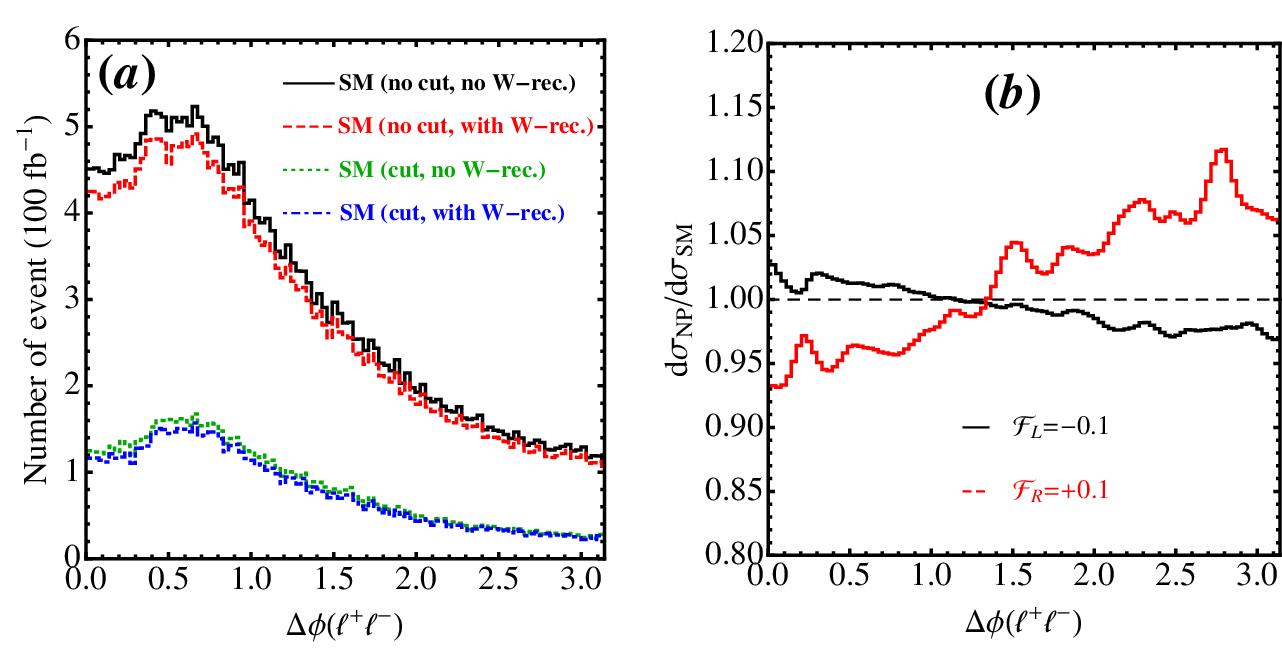
An observable is needed which changes shape in the presence of the anomalous couplings and . The opening angle between the two charged leptons from the boson decay in the transverse plane, , is such a candidate as is pointed out in Ref. [8]. Since pertains to the boson, it does not depend on the neutrino reconstruction. To illustrate this point, we plot the distribution in the SM in Fig. 4(a). Neutrino reconstruction reduces the number of observed events but does not change the shape of distribution. The kinematic cuts suppress the number of events but also do not change the shape.
The sensitivity of to the anomalous couplings is shown in Fig. 4(b) where we choose the somewhat generous values and for illustration. Note that values of this magnitude are not inconsistent with the Fermilab collider data on single top quark production, mentioned at the beginning of this section, although for such large and there must be additional contributions, other than those from the operators considered in Section II, in the precision electroweak measurements so as to relax the bounds in Fig. 1.

The top quark spin asymmetry is another observable sensitive to the anomalous couplings. At the LHC production proceeds predominately through the gluon fusion process . The presence of left- and right-handed couplings of the to the top quark in production means that parity is slightly broken, resulting in a small top quark spin asymmetry. The anomalous couplings and might amplify or weaken the parity violation effects, and a measurement of the asymmetry might provide a good probe for these anomalous couplings. Among the decay products of the top quark, the charged lepton is maximally correlated with the top quark spin [71, 72]. We can thus obtain the most distinctive distribution by plotting the angle between the spin axis and the charged lepton in the reconstructed top quark rest frame. Different choices of the reference frame to define the top quark polarization are found in the literature. In the helicity basis the top quark spin is measured along the top quark direction of motion in the center of mass (c.m.) frame. However, one must bear in mind that the anomalous couplings affect the production of the boson and top quark pair but not the top quark decay. Therefore, these couplings can be probed better in the spin correlation between the top quark decay products and the boson decay products. We find that the choice of the negatively charged lepton from the boson decay to measure the top quark spin direction amplifies the top quark spin correlation effects by almost a factor of 2.
In Fig. 5 we show the distribution for different spin bases, where is defined as
| (24) |
Here is the three-momentum of the top quark spin in the reconstructed c.m. frame, and is the charged lepton three-momentum defined in the rest frame of the top quark. In the helicity basis is chosen to be the direction of the top quark in the c.m. frame, while in the “optimal” basis is along the momentum of the negatively charged lepton from the boson decay in the top quark rest frame.
The angular distributions in Fig. 5(a,b) show a clear slope before reconstruction and kinematic cuts are imposed. However, the expected top quark spin correlations are diluted by the reconstruction of the neutrino momentum and the kinematic cuts, as shown in Fig. 5. Affected significantly by kinematic cuts, the top quark spin asymmetry seems not the best choice of variable for measuring the anomalous couplings. It may be of relevance only once LHC experiments reach a very high level of accuracy.
IV.4 Projected Bounds
IV.4.1 LHC Reach
We use the results of the event simulation outlined in Section IV B to derive projected bounds on deviations from the SM. The bounds are obtained here primarily from our fits to the distribution in . Our simulation is done at the leading order level. Theoretical uncertainties, arising from the uncalculated higher order corrections and from the parton distribution functions, should be included in order to make a fully realistic prediction. Next-to-leading order (NLO) QCD corrections reduce the renormalization/factorization scale dependence to after the choice of an appropriate scale [60], and they potentially affect final state differential distributions. While a detailed simulation at NLO is in order, it is beyond the scope of this work and we leave it to future work. Here, we conservatively consider an uncertainty of on our production estimates. The bounds will be improved when a more accurate NLO simulation is available.
In Fig. 6 we display the deviation of the cross section along one axis and the deviation of the single top quark production cross section along the other. Figure 6 (a) shows the projected C.L. bounds on the production cross section for integrated luminosities of (solid) and (dashed) at the LHC. The vertical bands denote the deviation of the single top quark production cross section: green for and blue for . The straight lines in Fig. 6(b) demonstrate the strong correlation between production and single top quark production induced by vanishing deviation of the coupling. The black solid line denotes , see Eq. (21). Non-zero will shift the curve up () or down (), see blue (red) lines.


The expectations of various new physics models are also plotted in Fig. 6(b). The top prime model [9] predictions are labeled by the (green) squares, where the mixing angle from top to bottom corresponding to , respectively. We also consider a right-handed model [10] in which only the right-handed coupling is modified. Its expectations are shown as the (purple) stars, where the mixing angle from top to bottom corresponding to , respectively. Another model includes a sequential fourth generation [11] whose quarks mix substantially with the third family. Both the and the couplings are modified by mass mixing of the top quark and fourth generation up-type quark (). One has to assume no mixing of the bottom quark in order to protect the coupling. When and are degenerate as it would be true in our effective operator framework, , shown as the (black) triangles, () from top to bottom.
Figure 6 is made under the assumption that the relation in Eq. (13) is valid. If instead one is interested checking Eq. (13) as a prediction of symmetry, one has to measure and to a high precision from two independent measurements, in order to verify . Such measurements may have to await a LC where one can measure the top quark polarization by choosing the polarization of the incoming electron beam. Since the SM gauge symmetry is well-established so far, we simply invoke Eq. (13) to analyze data at the LHC. One can still gain important information at the LHC:
- •
Assuming , one can use the single top quark production measurement to determine . Then can be determined from the total cross-section measurement uniquely.
- •
If and are measured from the differential distributions in production, one could then disentangle from in single top quark production. This result could allow us to determine whether .
- •
The sign of the anomalous couplings as determined by the LHC data could carry important information in terms of distinguishing different classes of models. For example, if the anomalous couplings are induced by the mixing of SM particles with heavy exotic particles, then the sign is negative (relative to the SM coupling) due to the mixing matrix. Observation of a positive anomalous coupling would imply that either the new physics model is a strongly interacting theory or the third generation quarks are in a higher representation of the SM gauge group [25].
It is convenient to summarize the above results in the plane of anomalous couplings and as shown in Fig. 7. The new physics models discussed above are distributed in different regions in the plot.
IV.4.2 Linear Collider Reach
Here we comment briefly on the reach in a linear collider. The anomalous coupling could be measured in at a high energy electron-positron linear collider. Our LHC results in Fig. 6(a) may be compared with expectations presented in the American Linear Collider working group report [73] for a 500 GeV machine and 100 fb-1 luminosity. The electron beam is assumed to be polarized. It is estimated that and can be measured to and accuracy in production, and that can be measured to in single top quark production. The magenta band in Fig. 6(a) denotes the 1 standard deviation bound on the production cross section at a LC. Furthermore, a study of top quark anomalous coupling measurements via single top quark production at an electron-photon collider shows that can be measured to with 500 fb-1 in a TeV machine [74, 75]. The figures suggest that the LHC with can reach a similar accuracy in production, together with precise measurement of the single top quark production cross section, as a LC ( and ).
As mentioned previously, such high precision at a linear collider could allow us to test the relation in Eq. (13) as a prediction of the electroweak symmetry, if one examines sufficiently many differential observables. In addition, the combination of data from the LHC and a LC may also allow for a precise determination of , which would not be possible using single top quark production alone.


Figure 7 shows that new physics cannot be tested or excluded beyond the level without violating the bound from current low energy precision data discussed in Sec. II.2. But one should keep in mind that the low energy electroweak bounds could be diluted by additional tree-level induced operators. Our collider simulation is based on only two effective couplings and does not depend on four-fermion operators, making it less model dependent. If no other operators are present, a significant increase of linear collider energy and improvement of detector acceptance would be needed in order to test new physics via correlations between the and couplings.
V Summary and Conclusions
In this paper we investigate correlations among the values of the , , and couplings. Two main contributions are made. First, we use a model-independent effective Lagrangian approach to parametrize the possible effects of new physics beyond the SM in terms of higher dimensional operators constructed from SM fields. We demonstrate that the symmetry of the SM yields correlations among the possible deviations of the , , and couplings. Imposing the stringent experimental bound on from data on and , we show that a unique prediction follows on the and couplings. The prediction is independent of the underlying new physics at the electroweak scale. We use existing experimental constraints to show that deviations of the and couplings from their SM values can depend on only two parameters, and , and we present the allowed ranges of these parameters for different new physics cutoff scales and Higgs boson masses.
In the second contribution in this paper, we study the prospects for determining and with LHC data. We focus on single top quark and associated production. Deviations from the SM of the single top quark total and differential cross sections depend only on , whereas the cross section for associated production is influenced by both and . We perform a detailed Monte Carlo simulation of the process, including the effects of experimental cuts. Among observables in that could be sensitive to the presence of and , we examine correlations between the top quark spin and the charged lepton from . We find that experimental cuts appear to leave a sample of effectively unpolarized top quarks, a disappointing conclusion that does not appear to have been established previously. Among the final state distributions in associated production, we confirm that the opening angle between the two charged leptons from the boson decay, , seems to be useful for limiting the couplings and . The principal results of our analysis are presented in Figs. 6 and 7 as a set of two-dimensional plots of the deviation from the SM of the associated production cross section versus the deviation of the single top quark cross section for integrated luminosities of and at the LHC. These expectations are contrasted with estimates for a high energy electron-positron linear collider (LC). A comparison is also shown with predictions based on a few recent models of new physics including a top-prime model [9], a right-handed model [10], and a model with sequential fourth generation quarks that mix with the third generation [11]. Our analysis suggests that about at the LHC would be needed to improve model independent constraints on and to the same level achievable at a 500 GeV LC with of integrated luminosity.
We also point out that the pattern of deviations predicted by the electroweak symmetry could allow us to separate the effect of the CKM element from that of the gauge coupling , which is also present in the matrix element. Measurements of the coupling could then be used as a constraint in analyses of data on single top quark production in order to determine . A non-zero would indicate non-unitarity of the CKM matrix and be a clear signal for physics beyond the SM.
Acknowledgements.
Q. H. C. is grateful to C.-P. Yuan for interesting and useful discussions. E. L. B. and I. L. are supported by the U. S. Department of Energy under Contract No. DE-AC02-06CH11357. Q. H. C. is supported in part by the Argonne National Laboratory and University of Chicago Joint Theory Institute (JTI) Grant 03921-07-137, and by the U.S. Department of Energy under Grants No. DE-AC02-06CH11357 and No. DE-FG02-90ER40560. I. L. also acknowledges the hospitality of the Aspen Center for Physics where part of this work was completed.References
- [1] DELPHI, J. Abdallah et al., Eur. Phys. J. C60, 1 (2009), arXiv:0901.4461.
- [2] D0, V. M. Abazov et al., Phys. Rev. Lett. 98, 181802 (2007), hep-ex/0612052.
- [3] D0, V. M. Abazov et al., (2009), arXiv:0903.0850.
- [4] CDF, T. Aaltonen et al., (2009), arXiv:0903.0885.
- [5] S. Weinberg, Physica A96, 327 (1979).
- [6] P. Meade and M. Reece, Phys. Rev. D74, 015010 (2006), arXiv:hep-ph/0601124.
- [7] Q.-H. Cao, C. S. Li, and C. P. Yuan, Phys. Lett. B668, 24 (2008), arXiv:hep-ph/0612243.
- [8] U. Baur, A. Juste, L. H. Orr, and D. Rainwater, Phys. Rev. D71, 054013 (2005), arXiv:hep-ph/0412021.
- [9] B. A. Dobrescu, K. Kong, and R. Mahbubani, (2009), arXiv:0902.0792.
- [10] R. S. Chivukula, B. A. Dobrescu, H. Georgi, and C. T. Hill, Phys. Rev. D59, 075003 (1999), arXiv:hep-ph/9809470.
- [11] G. D. Kribs, T. Plehn, M. Spannowsky, and T. M. P. Tait, Phys. Rev. D76, 075016 (2007), arXiv:0706.3718.
- [12] P. Batra and T. M. P. Tait, Phys. Rev. D74, 054021 (2006), arXiv:hep-ph/0606068.
- [13] W. Buchmuller and D. Wyler, Nucl. Phys. B268, 621 (1986).
- [14] C. Arzt, M. B. Einhorn, and J. Wudka, Nucl. Phys. B433, 41 (1995), hep-ph/9405214.
- [15] R. Barbieri, A. Pomarol, R. Rattazzi, and A. Strumia, Nucl. Phys. B703, 127 (2004), arXiv:hep-ph/0405040.
- [16] F. del Aguila, M. Perez-Victoria, and J. Santiago, Phys. Lett. B492, 98 (2000), arXiv:hep-ph/0007160.
- [17] F. del Aguila, M. Perez-Victoria, and J. Santiago, JHEP 09, 011 (2000), arXiv:hep-ph/0007316.
- [18] A. Manohar and H. Georgi, Nucl. Phys. B234, 189 (1984).
- [19] A. Strumia, Phys. Lett. B466, 107 (1999), arXiv:hep-ph/9906266.
- [20] K. G. Chetyrkin, M. Misiak, and M. Munz, Phys. Lett. B400, 206 (1997), hep-ph/9612313.
- [21] F. Larios, M. A. Perez, and C.-P. Yuan, Phys. Lett. B457, 334 (1999), hep-ph/9903394.
- [22] G. Burdman, M. C. Gonzalez-Garcia, and S. F. Novaes, Phys. Rev. D61, 114016 (2000), hep-ph/9906329.
- [23] B. Grzadkowski and M. Misiak, Phys. rev. D78, 077501 (2008), arXiv:0802.1413.
- [24] P. Sikivie, L. Susskind, M. B. Voloshin, and V. I. Zakharov, Nucl. Phys. B173, 189 (1980).
- [25] K. Agashe, R. Contino, L. Da Rold, and A. Pomarol, Phys. Lett. B641, 62 (2006), arXiv:hep-ph/0605341.
- [26] A. Pomarol and J. Serra, Phys. Rev. D78, 074026 (2008), arXiv:0806.3247.
- [27] D. O. Carlson, E. Malkawi, and C. P. Yuan, Phys. Lett. B337, 145 (1994), arXiv:hep-ph/9405277.
- [28] J. Alcaraz et al, (LEP Electroweak Working Group and the LEP Collaborations ALEPH, DELPHI, L3 and OPAL), (2005), arXiv:hep-ex/0511027.
- [29] G. Altarelli, (2004), arXiv:hep-ph/0406270.
- [30] G. Altarelli, R. Barbieri, and F. Caravaglios, Int. J. Mod. Phys. A13, 1031 (1998), arXiv:hep-ph/9712368.
- [31] D. Choudhury, T. M. P. Tait, and C. E. M. Wagner, Phys. Rev. D65, 053002 (2002), arXiv:hep-ph/0109097.
- [32] R. Contino, L. Da Rold, and A. Pomarol, Phys. Rev. D75, 055014 (2007), arXiv:hep-ph/0612048.
- [33] M. E. Albrecht, M. Blanke, A. J. Buras, B. Duling, and K. Gemmler, (2009), arXiv:0903.2415.
- [34] A. J. Buras, B. Duling, and S. Gori, (2009), arXiv:0905.2318.
- [35] N. Arkani-Hamed, A. G. Cohen, and H. Georgi, Phys. Lett. B513, 232 (2001), arXiv:hep-ph/0105239.
- [36] R. Contino, Y. Nomura, and A. Pomarol, Nucl. Phys. B671, 148 (2003), arXiv:hep-ph/0306259.
- [37] Z. Chacko, H.-S. Goh, and R. Harnik, Phys. Rev. Lett. 96, 231802 (2006), arXiv:hep-ph/0506256.
- [38] N. Arkani-Hamed, S. Dimopoulos, and G. R. Dvali, Phys. Lett. B429, 263 (1998), arXiv:hep-ph/9803315.
- [39] L. Randall and R. Sundrum, Phys. Rev. Lett. 83, 3370 (1999), arXiv:hep-ph/9905221.
- [40] G. L. Kane, G. A. Ladinsky, and C.-P. Yuan, Phys. Rev. D45, 124 (1992).
- [41] E. Malkawi and C. P. Yuan, Phys. Rev. D50, 4462 (1994), arXiv:hep-ph/9405322.
- [42] D. Espriu and J. Manzano, Phys. Rev. D65, 073005 (2002), hep-ph/0107112.
- [43] D. Espriu and J. Manzano, Phys. Rev. D66, 114009 (2002), hep-ph/0209030.
- [44] C.-R. Chen, F. Larios, and C.-P. Yuan, Phys. Lett. B631, 126 (2005), hep-ph/0503040.
- [45] J. Alwall et al., Eur. Phys. J. C49, 791 (2007), arXiv:hep-ph/0607115.
- [46] U. Baur, A. Juste, D. Rainwater, and L. H. Orr, Phys. Rev. D73, 034016 (2006), arXiv:hep-ph/0512262.
- [47] Z. Sullivan, Phys. Rev. D66, 075011 (2002), hep-ph/0207290.
- [48] J. Campbell, R. K. Ellis, and F. Tramontano, Phys. Rev. D70, 094012 (2004), hep-ph/0408158.
- [49] Q.-H. Cao and C.-P. Yuan, Phys. Rev. D71, 054022 (2005), hep-ph/0408180.
- [50] Z. Sullivan, Phys. Rev. D70, 114012 (2004), hep-ph/0408049.
- [51] S. Frixione, E. Laenen, P. Motylinski, and B. R. Webber, JHEP 03, 092 (2006), hep-ph/0512250.
- [52] Q.-H. Cao, R. Schwienhorst, and C.-P. Yuan, Phys. Rev. D71, 054023 (2005), hep-ph/0409040.
- [53] Z. Sullivan, Phys. Rev. D72, 094034 (2005), hep-ph/0510224.
- [54] J. Campbell and F. Tramontano, Nucl. Phys. B726, 109 (2005), hep-ph/0506289.
- [55] Q.-H. Cao, R. Schwienhorst, J. A. Benitez, R. Brock, and C.-P. Yuan, Phys. Rev. D72, 094027 (2005), hep-ph/0504230.
- [56] N. Kidonakis, Phys. Rev. D74, 114012 (2006), arXiv:hep-ph/0609287.
- [57] Q.-H. Cao, (2008), arXiv:0801.1539.
- [58] S. Frixione, E. Laenen, P. Motylinski, B. R. Webber, and C. D. White, JHEP 07, 029 (2008), arXiv:0805.3067.
- [59] J. M. Campbell, R. Frederix, F. Maltoni, and F. Tramontano, (2009), arXiv:0903.0005.
- [60] A. Lazopoulos, T. McElmurry, K. Melnikov, and F. Petriello, Phys. Lett. B666, 62 (2008), arXiv:0804.2220.
- [61] Z. Sullivan and E. L. Berger, Phys. Rev. D78, 034030 (2008), arXiv:0805.3720.
- [62] H.-C. Cheng and I. Low, JHEP 09, 051 (2003), arXiv:hep-ph/0308199.
- [63] I. Low, JHEP 10, 067 (2004), hep-ph/0409025.
- [64] H.-C. Cheng and I. Low, JHEP 08, 061 (2004), arXiv:hep-ph/0405243.
- [65] J. Hubisz and P. Meade, Phys. Rev. D71, 035016 (2005), hep-ph/0411264.
- [66] J. Hubisz, P. Meade, A. Noble, and M. Perelstein, JHEP 01, 135 (2006), hep-ph/0506042.
- [67] A. Belyaev, C.-R. Chen, K. Tobe, and C. P. Yuan, Phys. Rev. D74, 115020 (2006), arXiv:hep-ph/0609179.
- [68] Higgs Working Group, M. S. Carena et al., (2000), arXiv:hep-ph/0010338.
- [69] G. L. Kane and C.-P. Yuan, Phys. Rev. D40, 2231 (1989).
- [70] The Tevatron Electroweak Working Group, (2009), arXiv:0903.2503.
- [71] G. Mahlon and S. J. Parke, Phys. Rev. D53, 4886 (1996), hep-ph/9512264.
- [72] S. J. Parke and Y. Shadmi, Phys. Lett. B387, 199 (1996), hep-ph/9606419.
- [73] American Linear Collider Working Group, T. Abe et al., (2001), arXiv:hep-ex/0106057.
- [74] Q.-H. Cao and J. Wudka, Phys. Rev. D74, 094015 (2006), hep-ph/0608331.
- [75] B. Sahin and I. Sahin, Eur. Phys. J. C54, 435 (2008), arXiv:0709.0365.