Device independent state estimation based on Bell’s inequalities

As we said, we restrict to the case where the user applies only two measurement settings on each particle and the outcome is binary. In this case, there is only one Bell inequality, namely CHSH [9]. We further restrict our study in considering only the observed violation $S_{\mathrm{obs}}$ of CHSH as quantitative measure, being aware that the statistics $P(a,b|A,B)$ contain further information that might improve the estimates.

Since the source will be characterized by a single scalar quantity, the set of ideal states is the set of states $\boldsymbol{\Phi}$ such that $S=2\sqrt{2}$ is achievable. This set has been fully characterized [10, 11]: it consists of all pure states of the form $\sum_{j}c_{j}|\Psi_{j}\rangle$ where $|\Psi_{j}\rangle$ is a two-qubit maximally entangled state in a four-dimensional subspace, i.e., $|\Psi_{j}\rangle=\frac{1}{\sqrt{2}}(|2j-1,2j-1\rangle+|2j,2j\rangle)$ up to local unitaries. Since the relative phases of the $c_{j}$ do not play any role in the violation, we must add mixed states to the set. It is easy to verify that the most general such state can be written as $\boldsymbol{\Phi}=U_{A}U_{B}\boldsymbol{\Phi^{+}}\otimes\boldsymbol{\sigma}U_{A}^{\dagger}U_{B}^{\dagger}$ where $|\Phi^{+}\rangle=\frac{1}{\sqrt{2}}(|00\rangle+|11\rangle)$ is a two-qubit maximally entangled state, $\boldsymbol{\sigma}$ is an arbitrary state, and $U_{A}$, $U_{B}$ are arbitrary local unitaries. In their work on device-testing, Mayers and Yao (MY) [7] chose their reference states as those that could be written in the above form with $\boldsymbol{\sigma}$ pure, i.e., even though they did not refer to Bell inequalities, they where considering all pure states that violate CHSH maximally.

The distance between the actual source state, with density matrix $\boldsymbol{\rho}$, and the closest ideal state $\boldsymbol{\Phi}$, is conveniently measured by the trace distance [12, 13]:

where $\delta(\boldsymbol{\rho},\boldsymbol{\Phi})=\frac{1}{2}\,\mbox{Tr}|\boldsymbol{\rho}-\boldsymbol{\Phi}|$. The trace distance has a clear operational interpretation: in whatever task, $\boldsymbol{\rho}$ will behave differently from $\boldsymbol{\Phi}$ with probability at most $\delta(\boldsymbol{\rho},\boldsymbol{\Phi})$. In other words, the real source will differ from an ideal source with probability at most $\delta(\boldsymbol{\rho})$.

The problem we have set out to solve is thus to find a bound of the form

This bound can in principle be obtained by solving the following optimization problem:

where $S_{\mathrm{max}}(\boldsymbol{\rho})$ is the maximum CHSH violation that can be obtained by measuring state $\boldsymbol{\rho}$.

Deriving lower bounds, let alone tight lower bounds, for ${\cal D}_{MY}$ turns out to be much harder than we initially anticipated. In practice, it is simpler to work with the Fidelity rather than the trace distance, the two measures being related by $\delta\leq\sqrt{1-F}$ [13]. In analogy with eq. (1), we define

and one is then led to search for bounds of the form

For ${\cal F}_{MY}$ we obtain tight lower bounds if the state is restricted to consist of two qubits, or (modulo a conjecture of Gisin and Peres) if the state is restricted to be pure. Putting such hypotheses on the source goes against the philosophy of the black box scenario, but it allows us to get a mathematical grasp of the problem. When no restrictions are put on the state, we do not even have a lower bound on ${\cal F}_{MY}$ . However it is possible to introduce other notions of fidelity (see below) which have a clear operational meaning, and for which lower bounds can be computed without any hypothesis on the source.

Yet an alternative approach to the source characterization problem would consist in looking for a lower bound to the entanglement of the state $\boldsymbol{\rho}$:

where $E$ is an entanglement measure, such as the entanglement of formation, of distillation, etc… [14]. Below we obtain lower bounds on ${\cal E}$.

As a nontrivial warm up exercise, let us compute the bound eq. (5) under the assumption that the source emits a pair of qubits and that the measurements are von Neumann measurements. This is an undue restriction for the black-box scenario; we present this calculation because its result is interesting in itself, and will be an important tool for the main discussion.

In this case the set of ideal states is well known: only the maximally entangled states $\boldsymbol{\Phi}=U_{A}U_{B}\boldsymbol{\Phi^{+}}U_{A}^{\dagger}U_{B}^{\dagger}$ violate CHSH maximally. Therefore, $F_{MY}(\boldsymbol{\rho})=\max_{\boldsymbol{\Phi}}F(\boldsymbol{\rho},\boldsymbol{\Phi})$ reduces to the so called singlet fidelity of $\boldsymbol{\rho}$. Our approach consists in fixing the singlet fidelity of $\boldsymbol{\rho}$, and computing $S_{\mathrm{max}}(\boldsymbol{\rho})$. To this end we use the spectral decomposition of the Bell operator

First note that if $F(\boldsymbol{\rho})\leq\frac{1}{2}$ the state cannot be entangled, CHSH cannot be violated, and the bound $S_{\mathrm{max}}=2$ can be trivially achieved by the degenerate measurement $\hat{A}=\hat{A}^{\prime}=\hat{B}=\hat{B}^{\prime}=\hbox{\small 1\normalsize\kern-3.30002pt1}$. If the inequality is violated, the operators $\hat{A}$, $\hat{A}^{\prime}$, $\hat{B}$, and $\hat{B}^{\prime}$ must be linear combinations of the three Pauli matrices. Then the spectral decomposition $\hat{\mathcal{B}}=\sum_{i}\lambda_{i}|\Phi_{i}\rangle\langle\Phi_{i}|$ has the following properties [15]: the $|\Phi_{i}\rangle$ are a Bell basis (i.e., a basis of maximally entangled states) and the eigenvalues are $\{\lambda_{1},\lambda_{2},-\lambda_{2},-\lambda_{1}\}$ with $\mbox{Tr}(\hat{\mathcal{B}}^{2})=16$, i.e.,

which implies the Cirelson bound $|\lambda_{i}|\leq 2\sqrt{2}$ [16].

Therefore, for a given $\hat{\mathcal{B}}$ we have

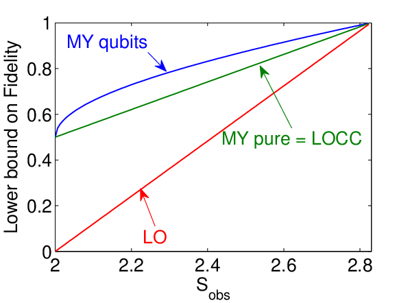
Suppose for definiteness $\lambda_{1}\geq\lambda_{2}\geq 0$. Then, keeping $F(\boldsymbol{\rho})$ fixed, $S(\boldsymbol{\rho})$ is maximized by choosing $|\Phi_{1}\rangle$ such that $F(\boldsymbol{\rho},\boldsymbol{\Phi_{1}})=F(\boldsymbol{\rho})$. Whereupon we have that $S_{\mathrm{max}}(\boldsymbol{\rho})\leq\lambda_{1}F(\boldsymbol{\rho})+\lambda_{2}(1-F(\boldsymbol{\rho}))$ because the two other eigenvalues are non-positive. Using eq. (8), we can set $\lambda_{1}=2\sqrt{2}\cos x$ and $\lambda_{2}=2\sqrt{2}\sin x$. The well-known bound $\max_{x}(a\cos x+b\sin x)=\sqrt{a^{2}+b^{2}}$ then leads to $S_{\mathrm{max}}(\boldsymbol{\rho})\leq 2\sqrt{2}\sqrt{F(\boldsymbol{\rho})^{2}+[1-F(\boldsymbol{\rho})]^{2}}$. Finally (Fig. 2):

This bound is tight, being achieved by pure non-maximally entangled states $|\psi\rangle=\cos\theta|00\rangle+\sin\theta|11\rangle$. Indeed, for these states $S_{\mathrm{max}}=2\sqrt{1+\sin^{2}(2\theta)}$ [17, 18] and the singlet fidelity is $F=\left|\langle\psi|\Phi^{+}\rangle\right|^{2}=\frac{1}{2}(1+\sin(2\theta))$. Furthermore for pairs of pure states, we have the strict equality $\delta=\sqrt{1-F}$, hence eq. (10) leads to a tight bound for the trace distance as well.

For any two dichotomic operators $\hat{A}$ and $\hat{A}^{\prime}$, one can find a basis such that both operators are block-diagonal, where each block is a $2\times 2$ matrix (see e.g. [3]). So one has $\hat{A}=\sum_{\alpha}\hat{A}_{\alpha}$ and $\hat{A}^{\prime}=\sum_{\alpha}\hat{A}^{\prime}_{\alpha}$ where $\hat{A}_{\alpha}=\Pi_{\alpha}\hat{A}\Pi_{\alpha}$, $\hat{A}^{\prime}_{\alpha}=\Pi_{\alpha}\hat{A}^{\prime}\Pi_{\alpha}$ and $\Pi_{\alpha}$ are orthogonal projectors onto 2 dimensional spaces. Of course, a similar decomposition holds for Bob’s operators. Therefore, the Bell-CHSH operator can be written as

where $\hat{\mathcal{B}}_{\alpha,\beta}=\sum_{i}\lambda_{i}^{\alpha\beta}|\Phi_{i}^{\alpha\beta}\rangle\langle\Phi_{i}^{\alpha\beta}|$ are orthogonal two-qubit operators with the same properties as above. Therefore

where $p_{\alpha\beta}\boldsymbol{\rho}_{\alpha\beta}=\Pi_{\alpha}\otimes\Pi_{\beta}{\boldsymbol{\rho}}\Pi_{\alpha}\otimes\Pi_{\beta}$ and $\boldsymbol{\rho}_{\alpha\beta}$ is a normalized two-qubit state.

Given (12), it may seem that the extension of our result to arbitrary dimensions is just a matter of convex optimization. A closer look shows that one must be much more careful, because the above construction does not imply:

where $F(\boldsymbol{\rho}_{\alpha\beta})$ is the singlet fidelity of $\boldsymbol{\rho}_{\alpha\beta}$. The reason is that in the MY approach, the state must be brought close to a reference state using local unitary operations $U_{A}\otimes U_{B}$. Let $U_{\alpha}$ be the restriction of $U_{A}$ to the $2\times 2$ block indexed by $\alpha$; and similarly for $U_{\beta}$; and let $\boldsymbol{\Phi}_{\alpha\beta}$ be the maximally entangled state of two qubit such that $F(\boldsymbol{\Phi}_{\alpha\beta},\boldsymbol{\rho}_{\alpha\beta})=F(\boldsymbol{\rho}_{\alpha\beta})$ is the singlet fidelity of $\boldsymbol{\rho}_{\alpha\beta}$. Now, there is no guarantee that $U_{A}$ and $U_{B}$ exist, such that $U_{\alpha}\otimes U_{\beta}\boldsymbol{\Phi}_{\alpha\beta}U_{\alpha}^{\dagger}\otimes U_{\beta}^{\dagger}=\boldsymbol{\Phi}^{+}$ for all $\alpha$ and $\beta$, as is required to obtain a reference state according to the MY definition. Moreover, the MY definition of fidelity is a comparison with the whole state $\boldsymbol{\Phi}^{+}\otimes\boldsymbol{\sigma}$, not only with the two-qubit component $\boldsymbol{\Phi}^{+}$. In order to make sense of eq. (13) we will introduce different definitions of fidelity below. Before turning to that, we present the case of pure states of arbitrary dimensions, for which the MY fidelity can be computed.

Let us assume that we know that the source emits a pure state (again an undue restriction for the black box scenario). Using the Schmidt decomposition $|\Psi\rangle=\sum_{k}\lambda_{k}|k,k\rangle$ with the Schmidt coefficients in decreasing order $\lambda_{k}\geq\lambda_{k+1}\geq 0$, any pure state can be rewritten as $|\Psi\rangle=\sum_{j}\sqrt{p_{j}}\left(c_{j}|2j,2j\rangle+s_{j}|2j+1,2j+1\rangle\right)$ with $c_{j}^{2}+s_{j}^{2}=1$. The MY fidelity can be computed exactly (Appendix A), and one finds

This should now be related to $S_{\mathrm{max}}(\Psi)$. For states of arbitrary dimension, there is no known analytical expression for the maximal violation of CHSH. However, for pure states $\Psi$ there is a long-standing conjecture by Gisin and Peres [19], whose validity has never been disproved by numerical checks [20]. According to this conjecture, the ordered Schmidt decomposition defines the natural block-structure of the CHSH operator. This implies

Combining this conjecture with eq. (14) we find that for pure states the accessible points in the $(F_{MY},S_{\mathrm{max}})$ plane are convex combinations of points on the curve given by equality in eq. (10), yielding (Fig. 2):

This bound is tight if we allow the dimension $d$ to become arbitrarily large (otherwise, the ordering of the $\lambda_{k}$ implies constraints on the possible values of $\{p_{j},c_{j},s_{j}\}$). Moreover, this bound is weaker than the one obtained under the assumption of two-qubits. Though not astonishing in itself, this feature is new: in device-independent quantum key distribution, the bound for collective attacks is already optimal in the two-qubit case [2, 3].

The MY fidelity is defined to suit the black-box scenario. However, other definitions of fidelity may be meaningful. Here, we consider fidelities defined as

where ${\cal L}$ is a set of completely positive maps which map the Hilbert space of $\boldsymbol{\rho}$ onto a $2\times 2$ dimensional Hilbert space, and which cannot increase the entanglement. $F_{\cal L}$ can be thought of as the best singlet fidelity obtainable under single shot purification of $\boldsymbol{\rho}$ to a two-qubit entangled state, using only operations that belong to the family ${\cal L}$. We will consider the case where ${\cal L}$ consists of all the completely positive maps that can be realised by Local Operations (${\cal L}=LO$) or by Local Operations and Classical Communication (${\cal L}=LOCC$).

These new notions of fidelity shed a different light on the task of source characterization. Indeed the Mayers-Yao fidelity and trace distance compare the state produced by the source to the closest ideal state, thereby establishing how much the real state and the idea state would differ in applications. The new fidlities $F_{\cal L}$ are relevant to another scenario in which the user may try to improve the source by acting locally on the two subsystems, for instance by opening the boxes containing the measurement devices and tinkering inside them. But before buying the source, the user wants to perform a fast black-box check to ascertain what will be the performance of the improved source. In other words, by measuring $S_{\mathrm{obs}}$ in a black-box scenario, the user can assess how well the source would perform in other scenarios. In this sense, the bounds we derive for these new fidelities are real black box statement, which do not make any hypothesis on the state $\boldsymbol{\rho}$ and on the measurement devices.

These new fidelities are related by

In Appendix B, we prove that $F_{MY}(\boldsymbol{\Psi})=F_{LO}(\boldsymbol{\Psi})$ for pure states while for mixed states there are explicit cases of strict inequality. We also show, see Fig. 2, that:

The bound (19) on $F_{LO}$ is obtained by exhibiting an explicit LO strategy. The proof is lengthy and we give it in Appendix C. We just note here that this bound is surely not tight, since it reaches the over-pessimistic $F=0$ for $S=2$.

The bound (20) for $F_{LOCC}$ is the same one obtained for $F_{MY}$ on pure states, eq. (16); we do not know whether this bound is tight. The proof goes as follows. The decomposition eq. (11) of the Bell-CHSH operator gives us a natural method for projecting $\boldsymbol{\rho}$ onto a 2 qubit space: particle A is projected in the $\Pi_{\alpha}$ spaces and particle B in the $\Pi_{\beta}$ spaces. Using CC, the actual block $(\alpha,\beta)$ is made known in both locations. The result of this completely positive map is a state with fidelity $F=p_{\alpha\beta}\sum_{\alpha\beta}F(\boldsymbol{\rho}_{\alpha\beta})$, i.e., we obtain a convex combination of points on the curve eq. (10). The bound (20) is recovered by noticing that, in the LOCC scenario, all the blocks $(\alpha,\beta)$ for which $S(\boldsymbol{\rho}_{\alpha\beta})=2$ can be brought to have $F=1/2$: indeed, for the blocks where they observe $S=2$, Alice and Bob can swap their local states with those of ancillas prepared in a pure product state.

Even if fidelity bounds were found to be tight, the tightness of the bound $\delta\leq\sqrt{1-F}$ on the trace distance would follow only if the states that saturate the bound are pure. However, we are already able to conclude that the bounds ${\cal D}(S_{\mathrm{obs}})$ for the trace distance $\delta$ put very stringent constraints on the quality of the source.

For instance, our strongest bound eq. (10) leads to a tight $\delta=\sqrt{1-F}$. If we insert $S_{\mathrm{obs}}=0.99\times 2\sqrt{2}$, we obtain $\delta\approx 10\%$. If the user requests the error rate to be below 1%, the vendor will have to produce extremely good sources — better than any currently available one.

The bounds for all the ${\cal F}_{\cal L}$ also provide lower bounds on the entanglement of $\boldsymbol{\rho}$. Indeed, consider any entanglement measure $E$ (see [14] for a list). By definition, ${\cal L}$ is a set of operations under which $E$ cannot increase; and the bounds on ${\cal F}_{\cal L}$ tell us how close the state $\boldsymbol{\rho}$ can be brought to the singlet state using only operations in ${\cal L}$. If ${\cal L}=LOCC$, each $\boldsymbol{\rho}_{\alpha\beta}$ can further be twirled, leading to the map $\boldsymbol{\boldsymbol{\rho}}\to p\,\boldsymbol{\Phi^{+}}+(1-p)\frac{\hbox{\small 1\normalsize\kern-3.30002pt1}}{4}$ with $p=\left(4{\cal F}_{LOCC}(S_{\mathrm{obs}})+1\right)/3$. For such states the entanglement measures can generally be computed. For instance, using [21], the entanglement of formation is bounded by

where $h$ is the binary entropy function.

References

- [1] J. F. Clauser, M. A. Horne, A. Shimony & R. A. Holt, Phys. Rev. Lett., 23, 880 (1969).
- [2] A. Acín, N. Brunner, N. Gisin, S. Massar, S. Pironio & V. Scarani, Phys. Rev. Lett. 98, 230501 (2007).
- [3] S. Pironio, A. Acín, N. Brunner, N. Gisin, S. Massar & V. Scarani, New J. Phys. 11, 045021 (2009).
- [4] N. Brunner, S. Pironio, A. Acín, N. Gisin, A. A. Méthot & V. Scarani, Phys. Rev. Lett. 100, 210503 (2008)
- [5] T. Vertesi & K. F. Pal, arXiv:0812.1572
- [6] J. Briet, H. Buhrman & B. Toner, arXiv:0901.2009
- [7] D. Mayers & A. Yao, Quantum Inform. Compu., 4, 273 (2004) [quant-ph/0307205].
- [8] F. Magniez, D. Mayers, M. Mosca & H. Ollivier, Self-testing of Quantum Circuits. In Proceedings of ICALP2006, Part I, M. Bugliesi et al. (Eds.), Lecture Notes in Computer Science 4051, pp. 72-83, 2006.
- [9] A. Fine, Phys. Rev. Lett. 48, 291 (1982)
- [10] S. L. Braunstein, A. Mann & M. Revzen, Phys. Rev. Lett. 68, 3259 (1992)
- [11] S. Popescu & D. Rohrlich, Phys. Lett. A 169, 411 (1992)
- [12] C. A. Fuchs & J. van der Graaf, IEEE T. Inform. Theory, 45, 1216 (1999) [quant-ph/9712042].
- [13] M. A. Nielsen & I. L. Chuang, Quantum Computation and Quantum Information (chap. 9), Cambridge University Press (2000).
- [14] R. Horodecki, P. Horodecki, M. Horodecki & K. Horodecki Rev. Mod. Phys. 81, 865 (2009)
- [15] V. Scarani & N. Gisin, J. Phys. A: Math. Gen. 34, 6043 (2001).
- [16] B. S. Cirel’son, Lett. Math. Phys., 4, 93 (1980).
- [17] R. F. Werner & M.M. Wolf, Quantum Information and Computation, 1, 1 (2001).
- [18] R. Horodecki, P. Horodecki & M. Horodecki, Phys. Lett. A, 200, 340 (1995).
- [19] N. Gisin & A. Peres, Phys. Lett. A 162, 15 (1992).
- [20] Y.-C. Liang & A. C. Doherty, Phys. Rev. A, 73, 052116 (2006).
- [21] C.H. Bennett, D.P. DiVincenzo, J.A. Smolin & W.K. Wootters, Phys. Rev. A, 54, 3824 (1996).