Spectrum Sensing by Cognitive Radios at Very Low SNR
Abstract
Spectrum sensing is one of the enabling functionalities for cognitive radio (CR) systems to operate in the spectrum white space. To protect the primary incumbent users from interference, the CR is required to detect incumbent signals at very low signal-to-noise ratio (SNR). In this paper, we present a spectrum sensing technique based on correlating spectra for detection of television (TV) broadcasting signals. The basic strategy is to correlate the periodogram of the received signal with the a priori known spectral features of the primary signal. We show that according to the Neyman-Pearson criterion, this spectra correlation-based sensing technique is asymptotically optimal at very low SNR and with a large sensing time. From the system design perspective, we analyze the effect of the spectral features on the spectrum sensing performance. Through the optimization analysis, we obtain useful insights on how to choose effective spectral features to achieve reliable sensing. Simulation results show that the proposed sensing technique can reliably detect analog and digital TV signals at SNR as low as dB.
Index Terms:
Spectrum sensing, distributed detection, adaptive filtering, and cognitive radio.I Introduction
Due to the increasing proliferation of wireless devices and services, the traditional static spectrum allocation policy becomes inefficient. The Federal Communications Commission (FCC) has recently opened the TV bands for cognitive radio devices, which can continuously sense the spectral environment, dynamically identify unused spectral segments, and then operate in these white spaces without causing harmful interference to the incumbent communication services [1]. The IEEE 802.22 Wireless Regional Area Network (WRAN) working group is developing a CR-based air interface standard for unlicensed operation in the unused TV bands [2].
Spectrum sensing to detect the presence of primary signals is one of the most important functionalities of CRs. To avoid causing harmful interference to the incumbent users, FCC requires that unlicensed CR devices operating in the unused TV bands detect TV and wireless microphone signals at a power level of dBm [1]. For a noise floor around dBm in the receiver circuitry (with respect to 6 MHz bandwidth and a 10 dB noise figure), spectrum sensing algorithms need to reliably detect incumbent TV signals at a very low SNR of at least dB. This requirement poses new challenges to the design of CR systems since traditional detection techniques such as energy detection and matched filtering are no longer applicable in the very low SNR region [2].
In general, there are three signal detection approaches for spectrum sensing: energy detection, matched filtering (coherent detection), and feature detection. If only the local noise power is known, the energy detector is optimal [3]. If a deterministic pattern (e.g., pilot, preamble, or training sequence) of primary signals is known, then the optimal detector usually applies a matched filtering structure to maximize the probability of detection. Depending on the available a priori information about the primary signal, one may choose one of the above approaches for spectrum sensing in CR networks. However, energy detection and matched filtering approaches are not applicable to detecting weak signals at very low SNR. At very low SNR, the energy detector suffers from noise uncertainty and the matched filter experiences the problem of lost synchronization. To improve sensing reliability, most previous studies have focused on the development of cooperative sensing schemes using multiple CRs [4][5][6]. An alternative approach is to use feature detection provided that some information is a priori known. Cyclostationary detection exploiting the periodicity in the modulated schemes [7] is such an example but requires high computational complexity. Recently, Zeng and Liang developed an eigenvalue based algorithm using the ratio of the maximum and minimum eigenvalues of the sample covariance matrix [8].
In this paper, we develop a feature detection-based spectrum sensing technique for a single CR to meet the FCC sensing requirement. The basic strategy is to correlate the periodogram of the received signal with the selected spectral features of a particular TV transmission scheme, either the national television system committee (NTSC) scheme or the advanced television standard committee (ATSC) scheme, and then to examine the correlation for decision making. By utilizing the asymptotic properties of Toeplitz matrices [9], we show that for certain signal models the spectra correlation-based detector is asymptotically equivalent to the likelihood ratio test (LRT) at very low SNR. In addition, we analyze how the spectral features can affect the sensing performance. Specifically, we formulate the sensing problem into an optimization problem. By solving this problem, we obtain useful insights on how to select or design effective spectral features to achieve reliable sensing. Extensive simulation results show that the proposed sensing technique can reliably detect TV signals from additive white Gaussian noise (AWGN) at SNR as low as dB.
II Spectra Correlation Based Spectrum Sensing
Before presenting the spectrum sensing technique, we first briefly review the TV transmission schemes.
II-A TV Signal Characteristics
A typical TV channel occupies a total bandwidth of MHz and its power spectrum density (PSD) describes how the signal power is distributed in the frequency domain. Fig. 1 (a) and (b) illustrate the PSD functions of both NTSC and ATSC signals. NTSC is the standardized analog video system used in North America and most of South America. The power spectrum of an NTSC signal consists of three peaks across the MHz channel, which correspond to the video, color, and audio carriers, respectively. On the other hand, ATSC is designed for the digital television (DTV) transmission, and it delivers a Moving Picture Experts Group (MPEG)-2 video stream of up to Mbps. The ATSC spectrum is relatively flat but has a pilot located in kHz above the lower edge of the channel.
We find that both NTSC and ATSC signals have distinct spectral features, which are constant during the transmissions. This observation motivates us to design a spectrum sensing technique for TV signals by exploiting these a priori known spectral features.


II-B Sensing Strategy
The spectrum sensing problem can be modeled into a binary hypothesis test at the -th time instant as follows:
| (1) |
where is the received signal by a secondary user, denotes the transmitted incumbent signal, and is assumed to be complex zero-mean additive white Gaussian noise (AWGN), i.e., . We assume that the signal and noise are independent. Accordingly, the PSD of the received signal for different hypotheses can be written as
| (2) |
where is the PSD function of the transmitted primary signal. Our objective is to distinguish between and by exploiting the unique spectral signature exhibited in .
Generally, we can obtain an estimate of the PSD of the observations through various spectral estimation algorithms, and here we focus on the periodogram, i.e., the squared magnitudes of the -point discrete-time Fourier transform (DFT) of the -point received signal, denoted
| (3) |
On the other hand, we suppose that the -point sampled PSD of the signal under detection, , is known a priori at the receiver. To detect the presence of a TV (NTSC or ATSC) signal, we perform the following test:
| (4) |
where is the decision threshold. Namely, if the spectra correlation between and is greater than the threshold then we would decide , i.e., presence of the signal of interest; otherwise, we would decide , i.e., absence of the primary signal.
III Asymptotic Optimality
In this section, we show that the proposed spectrum sensing technique (4) is asymptotically optimal at very low SNR in the Neyman-Pearson sense. The asymptotic optimality is in the sense that, as shown in Theorem 1 below, the decision statistic asymptotically approaches the likelihood ratio decision statistic for low SNR and large observation length.
III-A LRT at Very Low SNR
Considering a sensing interval of samples, we can represent the received signal and the primary transmitted signal in vector form as and . Since TV signals are perturbed by propagation along multiple paths, it may be reasonable to approximately model them as being a second-order stationary zero-mean Gaussian stochastic process, i.e,
| (5) |
where
| (6) |
is the covariance matrix. Consequently, (1) is equivalent to the following hypothesis testing problem in the -dimensional complex space :
| (7) |
where is the identity matrix. The logarithm of the likelihood ratio is given by [10]:
| (8) |
Incorporating the constant terms into the threshold, we obtain the logarithmic LRT detector in the quadratic form as
| (9) |
which is the optimal detection scheme according to the Neyman-Pearson criterion. This detector is also known as a quadratic detector.
From the Taylor series expansion, we have
| (10) |
where the convergence of the series is obtained if the eigenvalues of are less than unity. This condition always holds in the low SNR regime where grows sufficiently large. For weak signal detection in the very low SNR region, i.e., , (10) can be approximated as
| (11) |
Plugging (11) into (9), we obtain
Hence, the optimal LRT detector at very low SNR is given by
| (12) |
where .
III-B Asymptotic Equivalence
Now we show that our proposed spectra correlation-based detector (4) is asymptotically equivalent to the LRT detector at very low SNR (12). Consider a sequence of optimal LRT detectors as defined in (12)
| (13) |
Likewise, we define a sequence of spectra correlation detectors as
| (14) |
Note that the LRT detectors are performed in time domain while the spectra correlation detectors are in frequency domain. The asymptotic equivalence of these two sequences of detectors is established in the following theorem.
Theorem 1
Proof:
The proof is sketched in Appendix A. ∎
IV Spectral Feature Selection
In this section, we study the effect of spectral features on the detection performance. Although the sensing algorithm cannot control or change the spectral features of transmitted signals since these features are completely determined by the incumbent transmitter, we can obtain through analysis important insights to identify the best features for the signal detection. These insights are also useful for system engineers to design robust signals that can be reliably detected at very low SNR.
We first consider the case where there is no primary signal in the band of interest. Under hypothesis , we have
| (16) |
where
| (17) |
is the average power transmitted across the whole bandwidth. On the other hand, by exploiting the fact that the periodogram is an asymptotically unbiased estimate of the PSD [11], we have for sufficiently large ,
| (18) |
under hypothesis .
Here we shall use the difference between and to determine the detection performance. Suppose that we can control the spectral mask of the transmitted signal, we would like to maximize the difference between and , i.e.,
| (19) |
with the optimization variables . For large , this problem is equivalent to
| (20) |
which maximizes a convex function over a hyperplane. In the sequel, we will show how to solve this nonconvex optimization problem.
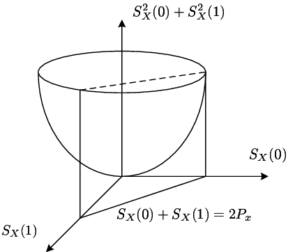
To solve (20), we first look at its geometrical representation, as shown in Fig. 2. It is easy to see that optimal solutions fall into the intersection of the convex surface of the objective function and the hyperplane determined by the constraints. Thus, the optimal solutions are given by
| (21) |
for any arbitrary , implying that all the transmit power is concentrated in a single frequency bin. Accordingly, the optimal value of (20) is
| (22) |
On the other hand, the worst case occurs when
| (23) |
which makes . In this extreme case, the spectral mask function is flat across the spectrum. A representative example of such a spectral feature is the white noise-like signal. This result is consistent with our intuition since it is generally difficult to distinguish a white Gaussian signal from additive white Gaussian noise. The optimal detector for such a case is the energy detector (radiometer) [10][3] provided that the noise power is perfectly known.
V Simulation Results
In this section, we numerically evaluate the proposed spectra feature correlation-based spectrum sensing algorithm for both ATSC and NTSC signals.
First, we obtain the “clean” baseband TV signals by capturing the TV signals in the RF front-end and then transforming the signals from the ultra-high frequency (UHF) bands to the baseband. Through processing, the TV signals in the baseband are sampled at a rate samples/sec, with MHz bandwidth. The TV data are divided into a number of blocks, each of which is msecs. The spectral features are obtained by computing the (averaged) periodograms of the clean TV signals.
We study the sensing performance for two channel models: AWGN and multipath fading. For the multipath fading channel model, we apply the ITU Pedestrian B model, whose power delay profile is given in Table I. The root mean square (RMS) delay spread of the ITU Ped-B model is ns. We pass the clean TV signals through the channel models to simulate the real wireless propagation environment.
| 0 | 200 | 800 | 1200 | 2300 | 3700 | |
|---|---|---|---|---|---|---|
| 0 | -0.9 | -4.9 | -8.0 | -7.8 | -23.9 |

For both ATSC and NTSC signals, we choose the test thresholds such that their false alarm rates are less than 0.001. We use the white Gaussian noise to test the sensing algorithms to make sure the false alarm rates are less than 0.001. Once we find the test thresholds for ATSC and NTSC signals, we can simulate and calculate the missed detection rates. For each SNR value, we simulate the sensing algorithms for 25,000 realizations. The simulation results for ATSC and NTSC are plotted in Figs. 3 and 4.
For both ATSC and NTSC signals, the spectral feature detector can reliably detect the signals at SNR dB with a missed detection rate less than in the AWGN channels. It can be observed that the NTSC signal is easier to detect than the ATSC signal since the NTSC signal has three sharp spectral features while the ATSC contains a large amount of flat spectrum and has only one feature corresponding to the pilot. This observation is consistent with our optimization analysis in Section IV.

VI Conclusion
In this paper, we have proposed a spectral feature detector for spectrum sensing in CR networks. The basic strategy is to use the correlation between the periodogram of the received signal and the a priori spectral features. Using the asymptotic properties of Toeplitz and circular matrices, we have shown that this spectral feature detector is asymptotically optimal at very low SNR and with a large block size. In addition, we have performed optimization analysis on the effects of spectral features on the sensing performance. The analytical results show that the signals with sharp spectral features are easier to detect compared with those with relatively flat spectra. The simulation results show that the proposed spectral feature correlation detector can reliably detect analog and digital TV signals at SNR as low as dB.
Appendix A Proof of Theorem 1
From the definition of the two test statistics, we have
| (24) |
where
| (25) |
is a diagonal matrix with the PSD of the incumbent signal in the diagonal, and is the DFT matrix defined as
| (26) |
with being a primitive th root of unity. Consequently,
| (27) |
where is a circular matrix. It has been shown in [9] that the Toepliz matrix is asymptotically equivalent to the circular matrix since the weak norm (Hilbert-Schmidt norm) of goes to zero [9], i.e.,
| (28) |
References
- [1] “Federal communications commission,” FCC-08-260, Nov. 2008. [Online]. Available: http://hraunfoss.fcc.gov/edocs_public/attachmatch/FCC-08-260A1.pdf.
- [2] S. Shellhammer, S. Shankar N, R. Tandra, and J. Tomcik, “Performance of power detector sensors of DTV signals in IEEE 802.22 WRANs,” in Proc. ACM TAPAS, Boston, MA, Aug. 2006.
- [3] S. M. Kay, Fundamentals of Statistical Signal Processing: Detection Theory. Prentice Hall, NJ, 1998.
- [4] Z. Quan, S. Cui, and A. H. Sayed, “Optimal linear cooperation for spectrum sensing in cognitive radio networks,” IEEE Journal of Selected Topics in Signal Processing, vol. 2, no. 1, pp. 28–40, Feb. 2008.
- [5] Z. Quan, S. Cui, H. V. Poor, and A. H. Sayed, “Collaborative wideband sensing for cognitive radios,” IEEE Signal Processing Magazine, no. 6, pp. 60–73, Nov. 2008.
- [6] Z. Quan, S. Cui, A. H. Sayed, and H. V. Poor, “Optimal multiband joint detection for spectrum sensing in cognitive radio networks,” IEEE Trans. Signal Processing, vol. 57, no. 3, pp. 1128–1140, Mar. 2009.
- [7] W. Gardner, “Exploitation of spectral redundancy in cyclostationary signals,” IEEE Signal Processing Mag., vol. 8, no. 2, pp. 14–36, Apr. 1991.
- [8] Y. Zeng and Y.-C. Liang, “Eigenvalue based spectrum sensing algorithms for cognitive radio,” IEEE Trans. Commun., to appear.
- [9] R. M. Gray, “Toeplitz and circular matrices: A review,” Foudations and Trends in Communications and Information Theory, vol. 2, no. 3, pp. 155–239, 2006.
- [10] H. V. Poor, An Introduction to Signal Detection and Estimation. Springer-Verlag, New York, 1994.
- [11] P. Stoica and R. L. Moses, Introduction to Spectral Analysis. Prentice Hall, 1997.