Law of the Minimum Paradoxes
Abstract
The “Law of the Minimum” states that growth is controlled by the scarcest resource (limiting factor). This concept was originally applied to plant or crop growth (Justus von Liebig, 1840 [1]) and quantitatively supported by many experiments. Some generalizations based on more complicated “dose-response” curves were proposed. Violations of this law in natural and experimental ecosystems were also reported. We study models of adaptation in ensembles of similar organisms under load of environmental factors and prove that violation of Liebig’s law follows from adaptation effects. If the fitness of an organism in a fixed environment satisfies the Law of the Minimum then adaptation equalizes the pressure of essential factors and therefore acts against the Liebig’s law. This is the the Law of the Minimum paradox: if for a randomly chosen pair “organism–environment” the Law of the Minimum typically holds, then, in a well-adapted system, we have to expect violations of this law.
For the opposite interaction of factors (a synergistic system of factors which amplify each other) adaptation leads from factor equivalence to limitations by a smaller number of factors.
For analysis of adaptation we develop a system of models based on Selye’s idea of the universal adaptation resource (adaptation energy). These models predict that under the load of an environmental factor a population separates into two groups (phases): a less correlated, well adapted group and a highly correlated group with a larger variance of attributes, which experiences problems with adaptation. Some empirical data are presented and evidences of interdisciplinary applications to econometrics are discussed.
Keywords: Liebig’s Law, Adaptation, Fitness, Stress
1 Introduction
1.1 The Law of the Minimum
The “Law of the Minimum” states that growth is controlled by the scarcest resource (limiting factor) [1]. This law is usually believed to be the result of Justus von Liebig’s research (1840) but the agronomist and chemist Carl Sprengel published in 1828 an article that contained in essence the Law of the Minimum and this law can be called the Sprengel–Liebig Law of the Minimum. [2].
This concept is illustrated in Fig. 1.

This concept was originally applied to plant or crop growth. Many times it was criticized, rejected, and then returned to and demonstrated quantitative agreement with experiments [1, 3, 4].
The Law of the Minimum was extended to a more general conception of factors, rather than for the elementary physical description of available chemical substances and energy. Any environmental factor essential for life that is below the critical minimum, or that exceeds the maximum tolerable level could be considered as a limiting one.
There were several attempts to create a general theory of factors and limitation in ecology, physiology and evolutionary biology. Tilman [5] proposed an equilibrium theory of resource competition based on classification of interaction in pairs of resources. They may be: (1) essential, (2) hemi-essential, (3) complementary, (4) perfectly substitutable, (5) antagonistic, or (6) switching. This interaction depends on spatial heterogeneity of resource distributions. For various resource types, the general criterion for stable coexistence of species was developed.
Bloom, Chapin and Mooney [7, 8] elaborated the economical metaphor of ecological concurrency. This analogy allowed them to merge the optimality and the limiting approach and to formulate four “theorems”. In particular, Theorem 3 states that a plant should adjust allocation so that, for a given expenditure in acquiring each resource, it achieves the same growth response: growth is equally limited by all resources. This is a result of adjustment: adaptation makes the limiting factors equally important. They also studied the possibility for resources to substitute for one another (Theorem 4) and introduced the concept of “exchange rate”.
For human physiology the observation that adaptation makes the limiting factors equally important was supported by many data of human adaptation to the Far North conditions (or, which is the same, disadaptation causes inequality of factors and leads to appearance of single limiting factor) [9]. The theory of factors – resource interaction was developed and supported by experimental data. The results are used for monitoring of human populations in Far North [10].
In their perspectives paper, Sih and Gleeson [11] considered three inter-related issues which form the core of evolutionary ecology: (1) key environmental factors; (2) organismal traits that are responses to the key factors; (3) the evolution of these key traits. They suggested to focus on ’limiting traits’ rather than optimal traits. Adaptation leads to optimality and equality of traits as well as of factors but under variations some traits should be more limiting than others. From the Sih and Gleeson point of view, there is a growing awareness of the potential value of the limiting traits approach as a guide for studies in both basic and applied ecology.
The critics of the Law of the Minimum is usually based on the “colimitation” phenomenon: limitation of growth and survival by a group of equally important factors and traits. For example, analysis of species-specific growth and mortality of juvenile trees at several contrasting sites suggests that light and other resources can be simultaneously limiting, and challenges the application of the Law of the Minimum to tree sapling growth [12].
The concept of multiple limitation was proposed for unicellular organisms based on the idea of the nutritional status of an organism expressed in terms of state variables [13]. The property of being limiting was defined in terms of the reserve surplus variables. This approach was illustrated by numerical experiments.
In the world oceans there are High Nutrient–Low Chlorophyll regions where chlorophyll concentrations are lower than expected concentrations given the ambient phosphate and nitrate levels. In these regions, limitations of phytoplankton growth by other nutrients like silicate or iron have been hypothesized and supported by experiments. This colimitation was studied using a nine-component ecosystem model embedded in the HAMOCC5 model of the oceanic carbon cycle [14].
The double–nutrient–limited growth appears also as a transition regime between two regimes with single limiting factor. For bacteria and yeasts at a constant dilution rate in the chemostat, three distinct growth regimes were recognized: (1) a clearly carbon-limited regime with the nitrogen source in excess, (2) a double–nutrient–limited growth regime where both the carbon and the nitrogen source were below the detection limit, and (3) a clearly nitrogen-limited growth regime with the carbon source in excess. The position of the double–nutrient–limited zone is very narrow at high growth rates and becomes broader during slow growth [15, 16].
Decomposition of soil organic matter is limited by both the available substrate and the active decomposer community. The colimitation effects strongly affect the feedbacks of soil carbon to global warming and its consequences [17].
Dynamics of communities lead to colimitation on community level even if organisms and populations remain limited by single factors. Communities are likely to adjust their stoichiometry by competitive exclusion and coexistence mechanisms. It guaranties simultaneous limitation by many resources and optimal use of them at the community scale. This conclusion was supported by a simple resource ratio model and an experimental test carried out in microcosms with bacteria [18].
In spite of the long previous discussion of colimitation, in 2008 Saito and Goepfert stressed that this notion is “an important yet often misunderstood concept” [20]. They describe the potential nutrient colimitation pairs in the marine environment and define three types of colimitation:
- I.
Independent nutrient colimitation concerns two elements that are generally biochemically mutually exclusive, but are also both found in such low concentrations as to be potentially limiting. Example: nitrogen–phosphorus colimitation.
- II.
Biochemical substitution colimitation involves two elements that can substitute for the same biochemical role within the organism. Example: zinc–cobalt colimitation.
- III.
Biochemically dependent colimitation refers to the limitation of one element that manifests itself in an inability to acquire another element. Example: zinc–carbon colimitation.
The experimental colimitation examples of the first type do not refute the Law of the Minimum completely but rather support the following statement: the ecological systems of various levels, from an organism to a community, may avoid the monolimitation regime either by the natural adjustment of their consumption structure [7, 19] or just by living in the transition zone between the monolimitation regimes. From the general point of view [11], such a transition zone is expected to be quite narrow (as a vicinity of a surface where factors are equal) but in some specific situations it may be broad, for example, for slow growth regimes in the chemostat [15, 16].
The type II and type III colimitations should be carefully separated from the usual discussion of the Law of the Minimum limitation. For these types of colimitation, two (or more) nutrients limit growth rates simultaneously, either through the effect of biochemical substitution (type II) or by depressing the ability for the uptake of another nutrient (type III) [20]. The type II and type III colimitations give us examples of the “non-Liebig” organization of the system of factors.
The Law of the Minimum is one of the most important tools for mathematical modeling of ecological systems. It gives a clue for constructing the first model for multi-component and multi-factor systems. This clue sounds rather simple: first of all, we have to take into account the most important factors which are, probably, limiting factors. Everything else should be excluded and allowed back only in a case when a “sufficient reason” is proved (following the famous “Principle of Sufficient Reason” by Leibnitz, one of the four recognized laws of thought).
It is suggested to consider the Liebig production function as the “archetype” for ecological modeling [21]. The generalizations of the Law of the Minimum were supported by the biochemical idea of limiting reaction steps (see, for example, [22] or recent review [23]). Three classical production functions, the Liebig, Mitscherlich and Liebscher relations between nutrient supply and crop production, are limiting cases of an integrated model based on the Michaelis–Menten kinetic equation [21].
Applications of the Law of the Minimum to the ecological modeling are very broad. The quantitative theories of the bottom–up control of the phytoplankton dynamics is based on the influence of limiting nutrients on growth and reproduction. The most used is the Droop model and its generalizations [24, 25, 26].
The Law of the Minimum was combined with the evolutionary dynamics to analyze the “Paradox of the plankton” [27] formulated by Hutchinson [28] in 1961: “How it is possible for a number of species to coexist in a relatively isotropic or unstructured environment all competing for the same sorts of materials… According to the principle of competitive exclusion… we should expect that one species alone would outcompete all of the others.” It was shown that evolution exacerbates the paradox and it is now very far from the resolution.
The theory of evolution from monolimitation toward colimitation was developed that takes into account the viruses attacks on the phytoplankton receptors [29]. In the classic theory [6], evolution toward colimitation decreases equilibrium resource concentrations and increases equilibrium population density. In contrary, under influence of viruses, evolution toward co-limitation may have no effect on equilibrium resource concentrations and may decreases the equilibrium population density [29].
The Law of the Minimum was used for modeling of microcolonial fungi growth on rock surfaces [30]. The analysis demonstrated, that a continued lack of organic nutrition is a dominating environmental factor limiting growth on stone monuments and other exposed rock surfaces in European temperate and Mediterranean climate.
McGill [31] developed a model of coevolution of mutualisms where one resource is traded for another resource. The mechanism is based on the Law of the Minimum in combination with Tilman’s approach to resource competition [5, 6]. It was shown that resource limitations cause mutualisms to have stable population dynamics.
The Law of the Minimum produces the piecewise linear growth functions which are non-smooth and very far from being linear. This nonlinearity transforms normal or uniform distributions of resource availabilities into skewed crop yield distribution and no natural satisfactory motivation exists in favor of any simple crop yield distribution [32]. With independent, identical, uniform resource availability distributions the yield skew is positive, and it is negative for normal distributions.
The standard linear tools of statistics such as generalized linear models do not work satisfactory for systems with limiting factors. Conventional correlation analysis conflicts with the concept of limiting factors. This was demonstrated in a study of the spatial distribution of Glacier lily in relation to soil properties and gopher disturbance [34]. For systems with limiting factors, quantile regression performs much better with strong theoretical justification in Law of the Minimum [33].
Some of the generalizations of the Law of the Minimum went quite far from agriculture and ecology. The Law of the Minimum was applied to economics [35] and to education, for example [36].
Recently, a strong mathematical background was created for the Law of the Minimum. Now the limiting factors theory together with static and dynamic limitation in chemical kinetics [23, 41] are considered as the realization of the Maslov dequantization [37, 38, 39] and idempotent analysis. Roughly speaking, the limiting factor formalism means that we should handle any two quantities either as equal numbers or as numbers connected by the relation : either or . Such a hard non-linearity can arise in the smooth dynamic models because of the time-scale separation [13].
Dequantization of the traditional mathematics leads to a mathematics over tropical algebras like the max-plus algebra. Since the classical work of Kleene [40] these algebras are intensively used in mathematics and computer science, and the concept of dequantization and idempotent analysis opened new applications in physics and other natural sciences (see the comprehensive introduction in [39]). Liebig’s and anti-Liebig’s (see Definition 1 below) systems of factors may be considered as realizations of max-plus or min-plus asymptotics correspondingly.
1.2 Fitness Convexity, Concavity and Various Interactions Between Factors
There exist an opposite type of organization of the system of factors, which, from a first glance, seems to be symmetric to Liebig’s type of interaction between them. In Liebig’s systems, the factor with the worst value determines the growth and surviving. The completely opposite situation is: the factor with the best value determines everything. We call such a system “anti-Liebig’s” one. Of course, it seems improbable that all the possible factors interact following the Law of the Minimum or the fully opposite anti-Liebig’s rule. Interactions between factors in real systems are much more complicated [20]. Nevertheless, we can state a question about hierarchical decomposition of the system of factors in elementary groups with simple interactions inside, then these elementary groups can be clustered into super–factors with simple interactions between them, and so on.
Let us introduce some notions and notations. We consider organisms that are under the influence of several factors . Each factor has its intensity (). For convenience, we consider all these factors as negative or harmful. This is just a convention about the choice of axes directions: a wholesome factor is just a “minus harmful” factor.
At this stage, we do not specify the nature of these factors. Formally, they are just inputs in the adaptation dynamics, the arguments of the fitness functions.
The fitness function is the central notion of the evolutionary and ecological dynamics. This is a function that maps the environmental factors and traits of the organism into the reproduction coefficient, that is, its contribution, in offspring to its population. Fisher proposed to construct fitness as a combination of independent individual contribution of various traits [42]. Haldane [43] criticized the approach based on independent actions of traits. Modern definitions of fitness function are based on adaptation dynamics. For the structured populations, the fitness should be defined through the dominant Lyapunov exponents [45, 44]. In the evolutionary game theory [46], payoff represents Darwinian fitness and describes how the use of the strategy improves an animal’s prospects for survival and reproduction. Recently, the Fisher and Haldane approaches are combined [47]: Haldane’s concern is incorporated into Fisher’s model by allowing the intensity of selection to vary between traits.
It is a nontrivial task to measure the fitness functions and action of selection in nature, but now it has been done for many populations and phenotypical traits [48]. Special statistical methods for life-history analysis for inference of fitness and population growth are developed and tested [49].
In our further analysis we do not need exact values of fitness but rather its existence and some qualitative features.
First of all, let us consider an oversimplified situation with identical organisms. Given phenotypical treats, fitness is a function of factor loads: . This assumption does not take into account physiological adaptation that works as a protection system and modifies the factor loads. This modification is in the focus of our analysis in the follow-up section, but for now we neglect adaptation. The convention about axes direction means that all the partial derivatives of are non-positive .
By definition, for a Liebig’s system of factors is a function of the worst (maximal) factor intensity: (Fig. 2a) and for anti-Liebig’s system it is the function of the best (minimal) factor intensity (Fig. 2c). Such representations as well as the usual formulation of the Law of the Minimum require special normalization of factor intensities to compare the loads of different factors.
For Liebig’s systems of factors the superlevel sets of given by inequalities are convex for any level in a convex domain (Fig. 2a). For anti-Liebig’s systems of factors the sublevel sets of given by inequalities are convex for any level in a convex domain (Fig. 2c).


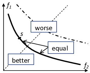
These convexity properties are essential for optimization problems which arise in the modeling of adaptation and evolution. Let us take them as definitions of the generalized Liebig and anti-Liebig systems of factors:
Definition 1
We call the generalized anti-Liebig systems of factors the synergistic systems because this formalizes the idea of synergy: in the synergistic systems harmful factors superlinear amplify each other.


Conditional maximization of fitness destroys the symmetry between Liebig’s and anti-Liebig’s systems as well as between generalized Liebig’s systems and synergistic ones. Following the geometric approach of [5, 6] we illustrate this optimization on Fig. 3. The picture may be quite different from the conditional maximization of a convex function near its minima point (compare, for example, Figs. 3c, 3d to Fig. from [11]).
Individual adaptation changes the picture. In the next subsection we discuss possible mechanism of these changes.
1.3 Adaptation Energy and Factor–Resource Models
The reaction of an organism to the load of a single factor may have plateaus (intervals of tolerance considered in Shelford’s “law of tolerance”, [69], Chapter 5). The dose–response curves may be nonmonotonic [50] or even oscillating. Nevertheless, we start from a very simple abstract model that is close to the usual factor analysis.
We consider organisms that are under the influence of several harmful factors with intensities (). Each organism has its adaptation systems, a “shield” that can decrease the influence of external factors. In the simplest case, it means that each system has an available adaptation resource, , which can be distributed for the neutralization of factors: instead of factor intensities the system is under pressure from factor values (where is the coefficient of efficiency of factor neutralization by the adaptation system and is the share of the adaptation resource assigned for the neutralization of factor , ). The zero value is optimal (the fully compensated factor), and further compensation is impossible and senseless.
For unambiguity of terminology, we use the term “factor” for all factors including any deficit of available external resource or even some illnesses. We keep the term “resource” for internal resources, mostly for the hypothetical Selye’s “adaptation energy”.
It should be specially stressed that the adaptation energy is neither physical energy nor a substance. This idealization describes the experimental results: in many experiments it was demonstrated, that organisms under load of various factors behave as if they spend a resource, which is the same for different factors. This resource may be exhausted and then the organism dies.
We represent the organisms, which are adapting to stress, as the systems which optimize distribution of available amount of a special adaptation resource for neutralization of different aggressive factors (we consider the deficit of anything necessary as a negative factor too). These factor–resource models with optimization are very convenient for the modeling of adaptation. We use a class of models many factors – one resource.
Interaction of each system with a factor is described by two quantities: the factor pressure and the resource assigned to the factor neutralization. The first quantity characterizes, how big the uncompensated harm is from that factor, the second quantity measures, how intensive is the adaptation answer to the factor (or how far the system was modified to answer the factor pressure).
Already one factor–one resource models of adaptation produce the tolerance law. We demonstrate below that it predicts the separation of groups of organism into two subgroups: the less correlated well–adapted organisms and highly correlated organisms with a deficit of the adaptation resource. The variance is also higher in the highly correlated group of organisms with a deficit of the adaptation resource.
This result has a clear geometric interpretation. Let us represent each organism as a data point in an -dimensional vector space. Assume that they fall roughly within an ellipsoid. The well-adapted organisms are not highly correlated and after normalization of scales to unit variance the corresponding cloud of points looks roughly as a sphere. The organisms with a deficit of the adaptation resource are highly correlated, hence in the same coordinates their cloud looks like an ellipsoid with remarkable eccentricity. Moreover, the largest diameter of this ellipsoid is larger than for the well–adapted organisms and the variance increases together with the correlations.
This increase of variance together with correlations may seem counterintuitive because it has no formal backgrounds in definitions of the correlation coefficients and variance. This is an empirical finding that under stress correlations and variance increase together, supported by many observations both for physiological and financial systems. The factor-resource models give a plausible explanation of this phenomena.
The crucial question is: what is the resource of adaptation? This question arose for the first time when Selye published the concept of adaptation energy and experimental evidence supporting this idea [51, 52]. Selye found that the organisms (rats) which demonstrate no differences in normal environment may differ significantly in adaptation to an increasing load of environmental factors. Moreover, when he repeated the experiments, he found that adaptation ability decreases after stress. All the observations could be explained by existence of an universal adaptation resource that is being spent during all adaptation processes.
Selye’s ideas allow the following interpretation: the aggressive influence of the environment on the organism may be represented as an action of independent factors. The system of adaptation consists of subsystems, which protect the organism from different factors. These subsystems consume the same resource, the adaptation energy. The distribution of this resource between the subsystems depends on environmental conditions.
Later the concept of adaptation energy was significantly improved [53], plenty of indirect evidence supporting this concept were found, but this elusive adaptation energy is still a theoretical concept, and in the modern “Encyclopedia of Stress” we read: “As for adaptation energy, Selye was never able to measure it…” [54]. Nevertheless, the notion of adaptation energy is very useful in the analysis of adaptation and is now in wide use (see, for example, [55, 56]).
The idea of exchange can help in the understanding of adaptation energy: there are many resources, but any resource can be exchanged for another one. To study such an exchange an analogy with the currency exchange is useful. Following this analogy, we have to specify, what is the exchange rate, how fast this exchange could be done (what is the exchange time), what is the margin, and how the margin depends on the exchange time. There may appear various limitations of the amount of the exchangeable resource, and so on. The economic metaphor for ecological concurrency and adaptation was elaborated in 1985 [7, 8] but much earlier, in 1952, it was developed for physiological adaptation [53].
Market economics seems closer to the idea of resource universalization than biology is, but for biology this exchange idea also seems useful. Of course there exist some limits on the possible exchanges of different resources. It is possible to include the exchange processes into models, but many questions arise about unknown coefficients. Nevertheless, we can follow Selye’s arguments and postulate the adaptation energy as a universal adaptation resource.
The adaptation energy is neither physical energy nor a substance. This is a theoretical construction, which may be considered as a pool of various exchangeable resources. When an organism achieves the limits of resource exchangeability, the universal non-specific stress and adaptation syndrome transforms (disintegrates) into specific diseases. Near this limit we have to expect the critical retardation [58] of exchange processes.
Adaptation optimizes the state of the system for given available amounts of the adaptation resource. This idea seems very natural, but it may be a difficult task to find the objective function that is hidden behind the adaptation process. Nevertheless, even an assumption about the existence of an objective function and about its general properties helps in analysis of adaptation process.
Assume that adaptation should maximize a fitness function which depends on the compensated values of factors, for the given amount of available resource:
| (1) |
The only question is: how can we be sure that adaptation follows any optimality principle? Existence of optimality is proven for microevolution processes and ecological succession. The mathematical backgrounds for the notion of “natural selection” in these situations are well–established after work by Haldane (1932) [43] and Gause (1934) [57]. Now this direction with various concepts of fitness (or “generalized fitness”) optimization is elaborated in many details (see, for example, review papers [59, 60, 61]).
The foundation of optimization is not so clear for such processes as modifications of a phenotype, and for adaptation in various time scales. The idea of genocopy–phenocopy interchangeability was formulated long ago by biologists to explain many experimental effects: the phenotype modifications simulate the optimal genotype ([63], p. 117). The idea of convergence of genetic and environmental effects was supported by an analysis of genome regulation [62] (the principle of concentration–affinity equivalence). The phenotype modifications produce the same change, as evolution of the genotype does, but faster and in a smaller range of conditions (the proper evolution can go further, but slower). It is natural to assume that adaptation in different time scales also follows the same direction, as evolution and phenotype modifications, but faster and for smaller changes. This hypothesis could be supported by many biological data and plausible reasoning. (See, for example, the case studies of relation between evolution of physiological adaptation [64, 65], a book about various mechanisms of plants responses to environmental stresses [66], a precise quantitative study of the relationship between evolutionary and physiological variation in hemoglobin [67] and a modern review with case studies [68].)
It may be a difficult task to find an explicit form of the fitness function , but for our qualitative analysis we need only a qualitative assumption about general properties of . First, we assume monotonicity with respect to each coordinate:
| (2) |
A system of factors is Liebig’s system, if
| (3) |
This means that fitness depends on the worst factor pressure.
A system of factors is generalized Liebig’s system (Definition 1.1), if for any two different vectors of factor pressures and () the value of fitness at the average point is greater, than at the worst of points , :
| (4) |
Any Liebig’s system is, at the same time, generalized Liebig’s system because for such a system the fitness is a decreasing function of the maximal factor pressure, the minimum of corresponds to the maximal value of the limiting factor and
The opposite principle of factor organization is synergy: the superlinear mutual amplification of factors. The system of factors is a synergistic one (Definition 1.2), if for any two different vectors of factor pressures and () the value of fitness at the average point is less, than at the best of points , :
| (5) |
A system of factors is anti-Liebig’s system, if
| (6) |
This means that fitness depends on the best factor pressure. Any anti-Liebig system is, at the same time a synergistic one because for such a system the fitness is a decreasing function of the minimal factor pressure, the maximum of corresponds to the minimal value of the factor with minimal pressure and
We prove that adaptation of an organism to Liebig’s system of factors, or to any synergistic system, leads to two paradoxes of adaptation:
- •
Law of the Minimum paradox (Sec. refSec:LawMinParad): If for a randomly selected pair, (State of environment – State of organism), the Law of the Minimum is valid (everything is limited by the factor with the worst value) then, after adaptation, many factors (the maximally possible amount of them) are equally important.
- •
Law of the Minimum inverse paradox (Sec. refSec:LawMinInvPar): If for a randomly selected pair, (State of environment – State of organism), many factors are equally important and superlinearly amplify each other then, after adaptation, a smaller amount of factors is important (everything is limited by the factors with the worst non-compensated values, the system approaches the Law of the Minimum).
In this paper, we discuss the individual adaptation. Other types of adaptations, such as changes of the ecosystem structure, ecological succession or microevolution lead to the same paradoxes if the factor–resource models are applicable to these processes.
2 One-Factor Models, the Law of Tolerance, and the Order–Disorder Transition
The question about interaction of various factors is very important, but, first of all, let us study the one-factor models. Each organism is characterized by measurable attributes and the value of adaptation resource, .
2.1 Tension–Driven Models
In these models, observable properties of interest can be modeled as functions of the pressure factor plus some noise .
Let us consider one-factor systems and linear functions (the simplest case). For the tension–driven model the attributes are linear functions of tension plus noise:
| (7) |
where is the expectation of for fully compensated factor, is a coefficient, , and is amount of available resource assigned for the factor neutralization. The values of could be considered as “normal” (in the sense opposite to “pathology”), and noise reflects variability of norm.
If systems compensate as much of factor value, as it is possible, then , and we can write:
| (8) |
Individual systems may be different by the value of factor intensity (the local intensity variability), by amount of available resource and, of course, by the random values of . If all systems have enough resource for the factor neutralization () then all the difference between them is in the noise variables . No change will observed under increase of the factor intensity, until violation of inequality occurs.
Let us define the dose–response curve as
Due to (7)
| (9) |
where is the probability of organism to have insufficient amount of resource for neutralization of the factor load and is the conditional expectation of the amount of resource if it is insufficient.
The slope of the dose–response curve (9) for big values of tends to , and for small it could be much smaller. This plateau at the beginning of the dose-response curve corresponds to the law of tolerance (V.E. Shelford, 1913, [69], Chapter 5).
If the factor value increases, and for some of the systems the factor intensity exceeds the available compensation then for these systems and the term in Eq. (7) becomes important. If the noise of the norm is independent of then the correlation between different increases monotonically with .
With increase of the factor intensity the dominant eigenvector of the correlation matrix between becomes more uniform in the coordinates, which tend asymptotically to .
For a given value of the factor intensity there are two groups of organisms: the well–adapted group with and , and the group of organisms with deficit of adaptation energy and . If the fluctuations of norm are independent for different (or just have small correlation coefficients), then in the group with deficit of adaptation energy the correlation between attributes is much higher than in the well–adapted group. If we use a metaphor from physics, we can call these two groups two phases: the highly correlated phase with deficit of adaptation energy and the less correlated phase of well-adapted organisms.
In this simple model (7) we just formalize Selye’s observations and theoretical argumentation. One can call it Selye’s model. There are two other clear possibilities for one factor–one resource models.
2.2 Response–Driven Models
What is more important for values of the observable quantities : the current pressure of the factors, or the adaptation to this factor which modified some of parameters? Perhaps, both, but let us introduce now the second simplest model.
In the response–driven model of adaptation, the quantities are modeled as linear functions of adaptive response (with coefficients ) plus some noise :
| (10) |
When increases then, after threshold , the term transforms into and does not change further. The observable quantities are not sensitive to changes in the factor intensity when is sufficiently large. This is the significant difference from the behavior of the tension-driven model (7), which is not sensitive to change of when is sufficiently small.
2.3 Tension–and–Response Driven 2D One–Factor Models
This model is just a linear combination of Eqs. (7) and (10)
| (11) |
For small (comfort zone) , the term vanishes, and the model has the form . For intermediate level of , if systems with both signs of inequality are present, the model imitates 2D (two-factor) behavior. After the threshold is passed for all systems, the model demonstrates 1D behavior again: For small the motion under change of goes along direction , for large it goes along direction .
Already the first model of adaptation (7) gives us the law of tolerance and practically important effect of order–disorder transition under stress. Now we have no arguments for decision which of these models is better, but the second model (10) has no tolerance plateau for small factor values, and the third model has almost two times more fitting parameters. Perhaps, the first choice should be the first model (7), with generalization to (11), if the described two-dimensional behaviour is observed.
3 Law of the Minimum Paradox
Liebig used the image of a barrel – now called Liebig’s barrel – to explain his law. Just as the capacity of a barrel with staves of unequal length is limited by the shortest stave, so a plant’s growth is limited by the nutrient in shortest supply.
Adaptation system acts as a cooper and repairs the shortest stave to improve the barrel capacity. Indeed, in well-adapted systems the limiting factor should be compensated as far as this is possible. It seems obvious because of the very natural idea of optimality, but arguments of this type in biology should be considered with care.
Assume that adaptation should maximize a objective function (1), which satisfies the Law of the Minimum (3) and the monotonicity requirement (2) under conditions , , . (Let us remind that for all .)
Description of the maximizers of gives the following theorem.
Theorem 3.1
For any objective function that satisfies conditions (3) the optimizers are defined by the following algorithm.
- 1.
Order intensities of factors: .
- 2.
Calculate differences (take formally ).
- 3.
Find such () that
For we put and if then we take .
- 4.
If then the optimal amount of resource is: for
(12) and for . If then for all .

Proof
This optimization is illustrated in Fig. 4. If then the pressure of all the factors could be compensated and we can take . Now, let us assume that . In this case, the pressure of some of the factors is not fully compensated. The adaptation resource is spent for partial compensation of the worst factors and the remained pressure of them is higher (or equal) then the pressure of the ()nd worst factor :
| (13) |
Therefore, for in the optimal distribution of the resource,
| (14) |
This gives us the first step in the Theorem 3.1, the definition of . Formula (12) for follows also from (13).
Hence, if the system satisfies the Law of the Minimum then the adaptation process makes the tension produced by different factors more uniform (Fig. 4). Thus adaptation decreases the effect from the limiting factor and hides manifestations of the Law of the Minimum.
Under the assumption of optimality (1) the Law of the Minimum paradox becomes a theorem: if the Law of the Minimum is true then microevolution, ecological succession, phenotype modifications and adaptation decrease the role of the limiting factors and bring the tension produced by different factors together.
The cooper starts to repair Liebig’s barrel from the shortest stave and after reparation the staves are more uniform, than they were before. This cooper may be microevolution, ecological succession, phenotype modifications, or adaptation. For the ecological succession this effect (the Law of the Minimum leads to its violation by succession) was described in Ref. [19]. For adaptation (and in general settings too) it was demonstrated in Ref. [9].
4 Law of the Minimum Inverse Paradox
The simplest formal example of “anti–Liebig’s” organization of interaction between factors gives us the following dependence of fitness from two factors: : each of factors is neutral in the absence of another factor, but together they are harmful. This is an example of synergy: the whole is greater than the sum of its parts. (For our selection of axes direction, “greater” means “more harm”.)
In according to Definition 1, the system of factors is synergistic, in a convex domain of the admissible vectors of factor pressure if for any level the sublevel set is convex. Another definition gives us the synergy inequality (5). These definitions are equivalent. This proposition follows from the definition of convexity and standard facts about convex sets (see, for example, [70])
Proposition 1
The synergy inequality (5) holds if and only if all the sublevel sets are strictly convex.
(The fitness itself may be a non-convex function.)
This proposition immediately implies that the synergy inequality is invariant with respect to increasing monotonic transformations of . This invariance with respect to nonlinear change of scale is very important, because usually we don’t know the values of function .
Proposition 2
If the synergy inequality (5) holds for a function , then it holds for a function , where is an arbitrary strictly monotonic function of one variable.
Already this property allows us to study the problem about optimal distribution of the adaptation resource without further knowledge about the fitness function.
Assume that adaptation should maximize an objective function (1) which satisfies the synergy inequality (5) under conditions , , . (Let us remind that for all .) Following our previous convention about axes directions all factors are harmful and is monotonically decreasing function (2). We need also a technical assumption that is defined on a convex set in and if it is defined for a nonnegative point , then it is also defined at any nonnegative point (this inequality means that for all ).
The set of possible maximizers is finite. For every group of factors (), , with the property
| (15) |
we find a distribution of resource :
| (16) |
This distribution (15) means that the pressure of factors are completely compensated and one factor is partially compensated. For , Eq. (15) gives and there exists only one nonzero component in the distribution (16), . For all , and all factors are fully compensated.
We get the following theorem as an application of standard results about extreme points of convex sets [70] to the monotonic function (2) with strictly convex sublevel sets.
Theorem 4.1
Any maximizer for under given conditions has the form (16).
To find the optimal distribution we have to analyze which distribution of the form (15) gives the highest fitness.
If the initial distribution of factors intensities, , is almost uniform and all factors are significant then, after adaptation, the distribution of effective tensions, (), is less uniform. Following Theorem 4.1, some of factors may be completely neutralized and one additional factor may be neutralized partially. This situation is opposite to adaptation to Liebig’s system of factors, where amount of significant factors increases and the distribution of tensions becomes more uniform because of adaptation. For Liebig’s system, adaptation transforms low dimensional picture (one limiting factor) into high dimensional one, and we expect the well-adapted systems have less correlations than in stress. For synergistic systems, adaptation transforms high dimensional picture into low dimensional one (less factors), and our expectations are inverse: we expect the well-adapted systems have more correlations than in stress (this situation is illustrated in Fig. 5; compare to Fig. 4). We call this property of adaptation to synergistic system of factors the Law of the Minimum inverse paradox.

The fitness by itself is a theoretical construction based on the average reproduction coefficient (instant fitness). It is impossible to measure this quantity in time intervals that are much shorter than the life length and even for the life–long analysis it is a non-trivial problem [49].
In order to understand which system of factors we deal with, Liebig’s or synergistic one, we have to compare theoretical consequences of their properties and compare them to empirical data. First of all, we can measure results of adaptation, and use for analysis properties of optimal adaptation in ensembles of systems for analysis (Fig. 4, Fig. 5).
5 Empirical data
In many areas of practice, from physiology to economics, psychology, and engineering we have to analyze the behavior of groups of many similar systems, which are adapting to the same or similar environment. Groups of humans in hard living conditions (Far North city, polar expedition, or a hospital, for example), trees under influence of anthropogenic air pollution, rats under poisoning, banks in financial crisis, enterprizes in recession, and many other situations of that type provide us with plenty of important problems, problems of diagnostics and prediction.
For many such situations it was found that the correlations between individual systems are better indicators than the value of attributes. More specifically, in thousands of experiments it was shown that in crisis, typically, even before obvious symptoms of crisis appear, the correlations increase, and, at the same time, the variance increase too. After the crisis achieves its bottom, it can develop into two directions: recovering (both the correlations and the variance decrease) or fatal catastrophe (the correlations decrease, but the variance continue to increase).
In this Sec. we review several sets of empirical results which demonstrate this effect. Now, after 21 years of studying this effect [9, 10], we maintain that this property is universal for groups of similar systems that are sustaining a stress and have an adaptation ability. On the other hand, situations with inverse behavior were predicted theoretically and found experimentally [71]. This makes the problem more intriguing.
Below, to collect information about strong correlations between many attributes in one indicator, we evaluate the non-diagonal part of the correlation matrix and delete terms with values below a threshold from the sum:
| (17) |
This quantity is a weight of the correlation graph. The vertices of this graph correspond to variables, and these vertices are connected by edges, if the absolute value of the correspondent sample correlation coefficient exceeds : . Usually, we take (a half of the maximum) if there is no reason to select another value.
5.1 Adaptation of Adults for Change of Climatic Zone
The activity of enzymes in human leukocytes was studied [72, 73] (alkaline phosphatase, acid phosphatase, succinate dehydrogenase, glyceraldehyde-3-phosphate dehydrogenase, glycerol- 3-phosphate dehydrogenase, and glucose-6-phosphate dehydrogenase).
We analyzed the short-term adaptation (20 days) of groups of healthy 20-30 year old men who change their climate zone:
- •
From the Far North to the South resort (Sochi, Black Sea) in the summer;
- •
From the temperate belt of Russia to the South resort (Sochi, Black Sea) in summer.
Results are represented in Fig. 6. This analysis supports the basic hypothesis and, on the other hand, could be used for prediction of the most dangerous periods in adaptation, which need special care.

We selected the group of 54 people who moved to the Far North, that had any illness during the period of short-term adaptation. After 6 months in the Far North, this test group demonstrates much higher correlations between activity of enzymes than the control group (98 people without illness during the adaptation period). For the activity of enzymes in leucocytes in the test group versus in the control group. To compare the dimensionless variance for these groups, we normalize the activity of enzymes to unite sample means (it is senseless to use the trace of the covariance matrix without normalization because normal activities of enzymes differ in order of magnitude). For the test group, the sum of the enzyme variances is 1.204, and for the control group it is 0.388.
5.2 Collapse of Correlations “on the Other Side of Crisis”: Acute Hemolytic Anemia in Mice
It is very important to understand where the system is going: (i) to the bottom of the crisis with possibility to recover after that bottom, (ii) to the normal state, from the bottom, or (iii) to the “no return” point, after which it cannot recover.
This problem was studied in many situations with analysis of fatal outcomes in oncological [74] and cardiological [75] clinics, and also in special experiments with acute hemolytic anemia caused by phenylhydrazine in mice [76]. The main result here is: when approaching the no-return point, correlations destroy ( decreases), and variance typically does continue to increase.
There exist no formal criterion to recognize the situation “on the other side of crisis”. Nevertheless, it is necessary to select situations for testing our hypothesis. Here the “general practitioner point of view” [53] can be of help. From such a point of view based on practical experience, the situation described below is on the other side of crisis: the acute hemolytic anemia caused by phenylhydrazine in mice with lethal outcome.

This effect was demonstrated in special experiments [76]. Acute hemolytic anemia caused by phenylhydrazine was studied in CBAxlac mice. Dynamics of correlation between hematocrit, reticulocytes, erythrocytes, and leukocytes in blood is presented in Fig. 7. After phenylhydrazine injections (60 mg/kg, twice a day, with interval 12 hours) during first 5-6 days the amount of red cells decreased (Fig. 7), but at the 7th and 8th days this amount increased because of spleen activity. After 8 days most of the mice died. Weight of the correlation graph increase precedeed the active adaptation response, but decreased to zero before death (Fig. 7), while amount of red cells increased also at the last day.
5.3 Grassy Plants Under Trampling Load
| Grassy Plant | Group 1 | Group 2 | Group 3 |
|---|---|---|---|
| Lamiastrum | 1.4 | 5.2 | 6.2 |
| Paris (quadrifolia) | 4.1 | 7.6 | 14.8 |
| Convallaria | 5.4 | 7.9 | 10.1 |
| Anemone | 8.1 | 12.5 | 15.8 |
| Pulmonaria | 8.8 | 11.9 | 15.1 |
| Asarum | 10.3 | 15.4 | 19.5 |
The effect exists for plants too. The grassy plants in oak tree-plants are studied [77]. For analysis the fragments of forests are selected, where the densities of trees and bushes were the same. The difference between those fragments was in damaging the soil surface by trampling. Three groups of fragments are studied:
- •
Group 1 – 0% of soil surface are destroyed by trampling;
- •
Group 2 – 25% of soil surface are destroyed by trampling;
- •
Group 3 – 70% of soil surface are destroyed by trampling.
The studied physiological attributes were: the height of sprouts, the length of roots, the diameter of roots, the amount of roots, the area of leafs, the area of roots. Results are presented in Table 1.
5.4 Scots Pines Near a Coal Power Station
The impact of emissions from a heat power station on Scots pine was studied [78]. For diagnostic purposes the secondary metabolites of phenolic nature were used. They are much more stable than the primary products and hold the information about past impact of environment on the plant organism for longer time.
The test group consisted of Scots pines (Pinus sylvestris L) in a 40 year old stand of the II class in the emission tongue 10 km from the power station. The station had been operating on brown coal for 45 years. The control group of Scots pines was from a stand of the same age and forest type, growing outside the industrial emission area. The needles for analysis were one year old from the shoots in the middle part of the crown. The samples were taken in spring during the bud swelling period. Individual composition of the alcohol extract of needles was studied by high efficiency liquid chromatography. 26 individual phenolic compounds were identified for all samples and used in analysis.
No reliable difference was found in the test group and control group average compositions. For example, the results for Proantocyanidin content (mg/g dry weight) were as follows:
- •
Total 37.43.2 (test) versus 36.82.0 (control);
Nevertheless, the variance of compositions of individual compounds in the test group was significantly higher, and the difference in correlations was huge: for the test group versus in the control group.
5.5 Choice of Coordinates and the Problem of Invariance
All indicators of the level of correlations are non-invariant with respect to transformations of coordinates. For example, rotation to the principal axis annuls all the correlations. Dynamics of variance also depends on nonlinear transformations of scales. Dimensionless variance of logarithms (or “relative variance”) often demonstrates more stable behavior especially when changes of mean values are large. The observed effect depends on the choice of attributes. Nevertheless, many researchers observed it without a special choice of coordinate system. What does it mean? We can propose a hypothesis: the effect may be so strong that it is almost improbable to select a coordinate system where it vanishes. For example, if one accepts the Selye model (7), (8) then observability of the effect means that for typical nonzero values of in crisis
| (18) |
for more than one value of , where var stands for variance of the noise component (this is sufficient for increase of the correlations). If
and the set of allowable transformations of coordinates is bounded (together with the set of inverse transformations), then the probability to select randomly a coordinate system which violates condition (18) is small (for reasonable definitions of this probability and of the relation ).
6 Comparison to Econometrics
The simplest Selye’s model (7) seems very similar to the classical one-factor econometrics models [79] which assume that the returns of stocks () are controlled by one factor, the “market” return . In this model, for any stock
| (19) |
where is the return of the th stock at time , and are real parameters, and is a zero mean noise. In our models, the pressure of factor characterizes the time window and is slower variable than the return.
The main difference between models (7) and (19) could be found in the nonlinear coupling (8) between the environmental property (the factor value ) and the property of individuals (the resource amount ). Exactly this coupling causes separation of a population into two groups: the well-adapted less correlated group and the highly correlated group with larger variances of individual properties and amount of resource which is not sufficient for compensation of the factor load. Let us check whether such a separation is valid for financial data.
6.1 Data Description
For the analysis of correlations in financial systems we used the daily closing values for companies that are registered in the FTSE 100 index (Financial Times Stock Exchange Index). The FTSE 100 is a market-capitalization weighted index representing the performance of the 100 largest UK-domiciled blue chip companies which pass screening for size and liquidity. The index represents approximately 88.03% of the UKs market capitalization. FTSE 100 constituents are all traded on the London Stock Exchanges SETS trading system. We selected 30 companies that had the highest value of the capital (on the 1st of January 2007) and stand for different types of business as well. The list of the companies and business types is displayed in Table 2.
| Number | Business type | Company | Abbreviation |
|---|---|---|---|
| 1 | Mining | Anglo American plc | AAL |
| 2 | BHP Billiton | BHP | |
| 3 | Energy (oil/gas) | BG Group | BG |
| 4 | BP | BP | |
| 5 | Royal Dutch Shell | RDSB | |
| 6 | Energy (distribution) | Centrica | CNA |
| 7 | National Grid | NG | |
| 8 | Finance (bank) | Barclays plc | BARC |
| 9 | HBOS | HBOS | |
| 10 | HSBC HLDG | HSBC | |
| 11 | Lloyds | LLOY | |
| 12 | Finance (insurance) | Admiral | ADM |
| 13 | Aviva | AV | |
| 14 | LandSecurities | LAND | |
| 15 | Prudential | PRU | |
| 16 | Standard Chartered | STAN | |
| 17 | Food production | Unilever | ULVR |
| 18 | Consumer | Diageo | DGE |
| 19 | goods/food/drinks | SABMiller | SAB |
| 20 | TESCO | TSCO | |
| 21 | Tobacco | British American Tobacco | BATS |
| 22 | Imperial Tobacco | IMT | |
| 23 | Pharmaceuticals | AstraZeneca | AZN |
| 24 | (inc. research) | GlaxoSmithKline | GSK |
| 25 | Telecommunications | BT Group | BTA |
| 26 | Vodafone | VOD | |
| 27 | Travel/leasure | Compass Group | CPG |
| 28 | Media (broadcasting) | British Sky Broadcasting | BSY |
| 29 | Aerospace/ | BAE System | BA |
| 30 | defence | Rolls-Royce | RR |
a) b)
b)
c)
d)
Data for these companies are available form the Yahoo!Finance web-site. For data cleaning we use also information for the selected period available at the London Stock Exchange web-site. Let denote the closing stock price for the th company at the moment , where , is the discrete time (the number of the trading day). We analyze the correlations of logarithmic returns: , in sliding time windows of length , this corresponds approximately to 4 weeks of 5 trading days. The correlation coefficients for time moment are calculated in the time window , which strongly precedes . Here we calculate correlations between individuals (stocks), and for biological data we calculated correlations between attributes. This corresponds to transposed data matrix.
6.2 Who Belongs to the Highly Correlated Group in Crisis
For analysis we selected the time interval 10/04/2006 - 21/07/2006 that represents the FTSE index decrease and restoration in spring and summer 2006 (more data are analyzed in our e-print [80]). In Fig. 8 the correlation graphs are presented for three time moments during the crisis development and three moments of the restoration. The vertices of this graph correspond to stocks. These vertices are connected by solid lines is the correspondent correlation coefficient , and by dashed lines if .
The correlation graphs from Fig. 8 show that in the development of this crisis (10/04/2006 - 21/07/2006) the correlated group was formed mostly by two clusters: a financial cluster (banks and insurance companies) and an energy (oil/gas) – mining – aerospace/defence and travel cluster. At the bottom of the crisis the correlated phase included almost all stocks. The recovery followed a significantly different trajectory: the correlated phase in the recovery seems absolutely different from that phase in the crisis development: there appeared the strong correlation between financial sector and industry. This is a sign that after the crisis bottom the simplest Selye’s model is not valid for a financial market. Perhaps, interaction between enterprizes and redistribution of resource between them should be taken into account. We need additional equations for dynamics of the available amounts of resource for th stock. Nevertheless, appearance of the highly correlated phase in the development of the crisis in the financial world followed the predictions of Selye’s model, at least, qualitatively.
Asymmetry between the drawups and the drawdowns of the financial market was noticed also in the analysis of the financial empirical correlation matrix of the 30 companies which compose the Deutsche Aktienindex (DAX) [81].
The market mode was studied by principal component analysis [82]. During periods of high market volatility values of the largest eigenvalue of the correlation matrix are large. This fact was commented as a strong collective behavior in regimes of high volatility. For this largest eigenvalue, the distribution of coordinates of the correspondent eigenvector has very remarkable properties:
- •
It is much more uniform than the prediction of the random matrix theory (authors of Ref. [82] described this vector as “approximately uniform”, suggesting that all stocks participate in this “market mode”);
- •
Almost all components of that eigenvector have the same sign.
- •
A large degree of cross correlations between stocks can be attributed to the influence of the largest eigenvalue and its corresponding eigenvector
Two interpretations of this eigenvector were proposed [82]: it corresponds either to the common strong factor that affects all stocks, or it represents the “collective response” of the entire market to stimuli. Our observation supports this conclusion at the bottom of the crisis. At the beginning of the crisis the correlated group includes stocks which are sensitive to the factor load, and other stocks are tolerant and form the less correlated group with the smaller variance. Following Selye’s model we can conclude that the effect is the result of nonlinear coupling of the environmental factor load and the individual adaptation response.
7 Functional Decomposition and Integration of Subsystems
In the simple factor–resource Selye models the adaptation response has no structure: the organism just distributes the adaptation resource to neutralization of various harmful factors. It is possible to make this model more realistic by decomposition. The resource is assigned not directly “against factors” but is used for activation and intensification of some subsystems.
We need to define the hierarchical structure of the organism to link the behavior in across multiple scales. In integrative and computational physiology it is necessary to go both bottom–up and top–up approaches. The bottom–up approach goes from proteins to cells, tissues, organs and organ systems, and finally to a whole organism [83].
The top-down approach starts from a bird’s eye view of the behavior of the system – from the top or the whole and aims to discover and characterize biological mechanisms closer to the bottom – that is, the parts and their interactions [83].
There is a long history of discussion of functional structure of the organism, and many approaches are developed: from the Anokhin theory of functional systems [84] to the inspired by the General Systems approach theory of “Formal Biological Systems” [85].
The notion of functional systems represents a special type of integration of physiological functions. Individual organs and tissue elements, are selectively combined into self-regulating systems organizations to achieve the necessary adaptive results important for the whole organism. The self-organization process is ruled by the adaptation needs.
For decomposition of the models of physiological systems, the concept of principal dynamic modes was developed [86, 87].
In this section, we demonstrate how to decompose the factor–resource models of the adaptation of the organism to subsystems.
In general, the analysis of interaction of factors is decomposed to interaction of factors and subsystems. Compensation of the harm from each factor requires activity of various systems. For every system a variable, activation level is defined. Level 0 corresponds to a fully disabled subsystem (and for most of essentially important subsystems it implies death). For each factor and every subsystem a “standard level” of activity is defined. Roughly speaking, this level of activation of the subsystem is necessary for neutralization of the unit value of the pressure of the factor . If then the subsystem is not involved in the neutralization of the factor .
In this model resources are assigned not to neutralization of factors but for activation of subsystems. The activation intensity of the subsystem depends on the adaptation resource , assigned to this subsystem:
| (21) |
For any given organization of the system of factors, optimization of fitness together with definitions (20) and (21) lead to a clearly stated optimization problem. For example, for Liebig’s system of factors we have to find distributions of that give solution to a problem:
| (22) |
If this minimum of maxima is positive () then the optimal distribution of resources is unique. If then there exists a polyhedron of optimal distributions given by the system of inequalities:
For the study of integration in experiment we use principal component analysis and find, parameters of which systems give significant inputs in the first principal components. Under the stress, the configuration of the subsystems, which are significantly involved in the first principal components, changes [88].
We analyzed interaction of cardiovascular and respiratory subsystems under exercise tolerance tests at various levels of load. Typically, we observe the following dynamics of the first factor composition. With increase of the load, coordinates both the correlations of the subsystems attributes with the first factor increase up to some maximal load which depend on the age and the health in the group of patients. After this maximum of integration, if the load continues to increase then the level of integration decreases [88].
Generalization of Selye’s models by decomposition creates a rich and flexible system of models for adaptation of hierarchically organized systems. Principal component analysis [89] with its various nonlinear generalizations [90, 91] gives a system of tools for extracting the information about integration of subsystems from the empirical data.
8 Conclusion
Due to the Law of the Minimum paradoxes, if we observe the Law of the Minimum in artificial systems, then under natural conditions adaptation will equalize the load of different factors and we can expect a violation of the Law of the Minimum. Inversely, if an artificial systems demonstrate significant violation of the law of the minimum, then we can expect that under natural conditions adaptation will compensate this violation.
This effect follows from the factor–resource models of adaptation and the idea of optimality applied to these models. We don’t need an explicit form of generalized fitness (which may be difficult to find), but use only the general properties that follow from the Law of the Minimum (or, oppositely, from the assumption of synergy).
Another consequence of the factor–resource models is the prediction of the appearance of strongly correlated groups of individuals under an increase of the load of environmental factors. Higher correlations in those groups do not mean that individuals become more similar, because the variance in those groups is also higher. This effect is observed for financial market too and seems to be very general in ensembles of systems which are adapting to environmental factors load.
Decomposition of the factor–resource models for the hierarchy of subsystems allows us to discuss integration of the subsystems in adaptation. For the explorative analysis of this integration in empirical data the principal component analysis is the first choice: for the high level of integration different subsystems join in the main factors.
The most important shortcoming of the factor–resource models is the lack of dynamics. In the present form it describes adaptation as a single action, the distribution of the adaptation resource. We avoid any kinetic modeling. Nevertheless, adaptation is a process in time. We have to create a system of dynamical models.
References
- (1) F. Salisbury (1992) Plant physiology (4th ed.), Wadsworth, Belmont, CA.
- (2) R.R. van der Ploeg, W. Böhm, M.B. Kirkham, (1999), On the origin of the theory of mineral nutrition of plants and the law of the minimum, Soil Science Society of America Journal 63, 1055–1062.
- (3) Q. Paris, (1992), The Return of von Liebig’s “Law of the Minimum”, Agron. J., 84, 1040–1046
- (4) B.S. Cade, J.W. Terrell, R.L. Schroeder, (1999), Estimating effects of limiting factors with regression quantiles, Ecology 80 (1), 311–323.
- (5) D. Tilman, (1980), Resources: a graphical-mechanistic approach to competition and predation, Am. Nat. 116 (3), 362–393.
- (6) D. Tilman (1982) Resource Competition and Community Structure, Princeton University Press, Princeton, NJ.
- (7) A.J. Bloom, F.S. Chapin III, H.A. Mooney, (1985), Resource limitation in plants – an economic analogy. Annu. Rev. Ecol. Syst. 16, 363–392.
- (8) F.S. Chapin, III, E. Schulze, H.A. Mooney, (1990), The Ecology and Economics of Storage in Plants, Annu. Rev. Ecol. Syst. 21, 423–447.
- (9) A.N. Gorban, V.T. Manchuk, E.V. Petushkova (Smirnova) (1987) Dynamics of physiological paramethers correlations and the ecological-evolutionary principle of polyfactoriality, In: Problemy Ekologicheskogo Monitoringa i Modelirovaniya Ekosistem [The Problems of Ecological Monitoring and Ecosystem Modelling], Vol. 10. Gidrometeoizdat, Leningrad, pp. 187–198.
- (10) K.R. Sedov, A.N. Gorban’, E.V. Petushkova (Smirnova), V.T. Manchuk, E.N. Shalamova, (1988), Correlation adaptometry as a method of screening of the population, Vestn Akad Med Nauk SSSR (10), 69–75. PMID: 3223045
- (11) A. Sih, S.K. Gleeson, (1995), A limits-oriented approach to evolutionary ecology, Trends in Ecology and Evolution 10 (9), 378–382.
- (12) R.K. Kobe (1996) Intraspecific Variation in Sapling Mortality and Growth Predicts Geographic Variation in Forest Composition, In: Ecological Monographs: Vol. 66 (2), pp. 181–201.
- (13) H.A. van den Berg, (1998), Multiple nutrient limitation in unicellulars: reconstructing Liebig’s law, Mathematical Biosciences, 149 (1), 1–22.
- (14) O. Aumont, E. Maier-Reimer, S. Blain, P. Monfray, (2003), An ecosystem model of the global ocean including Fe, Si, P colimitations, Global Biogeochemical Cycles 17 (2), 1060, doi:10.1029/2001GB001745.
- (15) T. Egli, M. Zinn, (2003), The concept of multiple-nutrient-limited growth of microorganisms and its application in biotechnological processes, Biotechnology Advances 22 (1-2), 35–43
- (16) M. Zinn, B. Witholt, T. Egli, (2004), Dual nutrient limited growth: models, experimental observations, and applications, Journal of Biotechnology 113 (1-3), 263–279.
- (17) T. Wutzler and M. Reichstein, (2008), Colimitation of decomposition by substrate and decomposers – a comparison of model formulations, Biogeosciences Discuss. 5, 163–190.
- (18) M. Danger, T. Daufresne, F. Lucas, S. Pissard, G. Lacroix, (2008), Does Liebig’s law of the minimum scale up from species to communities? Oikos 117 (11), 1741–1751
- (19) F.N. Semevsky, S.M. Semenov (1982) Mathematical modeling of ecological processes, Gidrometeoizdat, Leningrad.
- (20) M.A. Saito, T.J. Goepfert, (2008), Some thoughts on the concept of colimitation: Three definitions and the importance of bioavailability, Limnol. Oceanogr. 53 (1), 276–290
- (21) G.O. Nijland, J. Schouls, J. Goudriaan, (2008), Integrating the production functions of Liebig, Michaelis-Menten, Mitscherlich and Liebscher into one system dynamics model, NJAS - Wageningen Journal of Life Sciences 55 (2), 199–224.
- (22) G. C. Brown and C. E. Cooper, (1993). Control analysis applied to a single enzymes: can an isolated enzyme have a unique rate–limiting step? Biochem. J. 294, 87–94.
- (23) A.N. Gorban, O. Radulescu, (2008), Dynamic and Static Limitation in Multiscale Reaction Networks, Revisited, Advances in Chemical Engineering 34, 103–173.
- (24) M.R. Droop, (1973), Some thoughts on nutrient limitation in algae, J. Phycol. 9, 264–272.
- (25) T. Legović, A. Cruzado, (1997), A model of phytoplankton growth on multiple nutrients based on the Michaelis-Menten-Monod uptake, Droop’s growth and Liebig’s law, Ecol. Modelling 99 (1), 19–31.
- (26) F. Ballantyne IV., D.N.L. Menge, A. Ostling and P. Hosseini, (2008), Nutrient recycling affects autotroph and ecosystem stoichiometry, Am. Nat. 171 (4), 511–523.
- (27) N. Shoresh, M. Hegreness, R. Kishony, (2008), Evolution exacerbates the paradox of the plankton, PNAS USA 105 (34), 12365–12369.
- (28) G.E. Hutchinson, (1961), The paradox of the plankton, Am. Nat. 95, 137–145.
- (29) D.N.L. Menge, J.S. Weitz, (2009), Dangerous nutrients: Evolution of phytoplankton resource uptake subject to virus attack, Journal of Theoretical Biology, 257 (1), 104–115.
- (30) O. Chertov, A. Gorbushina, B. Deventer, (2004), A model for microcolonial fungi growth on rock surfaces, Ecological Modelling 177 (3-4), 415–426.
- (31) B. McGill, (2005), A mechanistic model of a mutualism and its ecological and evolutionary dynamics, Ecological Modelling 187 (4), Pages 413–425.
- (32) D.A. Hennessy, (2009), Crop yield skewness under law of the minimum technology, American Journal of Agricultural Economics 91 (1), 197–208.
- (33) M. Austin, (2007), Species distribution models and ecological theory: A critical assessment and some possible new approaches, Ecological Modelling 200 (1-2), 1–19.
- (34) J.D. Thomson, G. Weiblen, B.A. Thomson, S. Alfaro, P. Legendre, (1996), Untangling multiple factors in spatial distributions: lilies, gophers and rocks, Ecology 77, 16981715.
- (35) H.E. Daly, (1991), Population and Economics – A Bioeconomic Analysis, Population and Environment 12 (3), 257–263.
- (36) M.Y. Ozden, (2004), Law of the Minimum in Learning, Educational Technology & Society 7 (3), 5–8.
- (37) V. Kolokoltsov, V. Maslov (1997) Idempotent analysis and applications, Kluwer Acad. Publ., Dordrecht.
- (38) G.L. Litvinov, V.P. Maslov (Eds.) (2005) Idempotent mathematics and mathematical physics, Contemporary Mathematics, Vol. 377, AMS, Providence, RI.
- (39) G.L. Litvinov, (2007), The Maslov dequantization, idempotent and tropical mathematics: a brief introduction, Journal of Mathematical Sciences 140 (3), 426-444. E-print: arXiv:math/0507014 [math.GM].
- (40) S.C. Kleene (1956) Representation of events in nerve sets and finite automata, In: J. McCarthy and C. Shannon (Eds), Automata Studies, Princeton University Press, Princeton, pp. 3–40.
- (41) A.N. Gorban, O. Radulescu, A.Y. Zinovyev, (2010), Asymptotology of chemical reaction networks, Chem. Eng. Sci. 65, 2310–2324.
- (42) R.A. Fisher (1930) The genetical theory of natural selection, Oxford University Press, Oxford.
- (43) J.B.S. Haldane (1932) The causes of evolution, Longmans Green, London.
- (44) J.A.J. Metz, R.M. Nisbet, S.A.H. Geritz, (1992), How should we define fitness for general ecological scenarios, Trends Ecol. Evol. 7, 198–202.
- (45) A.N. Gorban (1984) Equilibrium encircling. Equations of chemical kinetics and their thermodynamic analysis, Nauka, Novosibirsk.
- (46) J. Maynard-Smith (1982) Evolution and the Theory of Games, Cambridge University Press, Cambridge.
- (47) D. Waxman, J.J. Welch, (2005), Fisher’s Microscope and Haldane’s Ellipse, Am. Nat. 166, 447–457.
- (48) J.G. Kingsolver, D.W. Pfennig, (2007), Patterns and Power of Phenotypic Selection in Nature, BioScience 57 (7), 561–572.
- (49) R.G. Shaw, C.J. Geyer, S. Wagenius, H.H. Hangelbroek, J.R. Etterson, (2008), Unifying Life-History Analyses for Inference of Fitness and Population Growth, Am. Nat. 172, E35–E47.
- (50) T. Colborn, D. Dumanoski, J.P. Meyers (1996) Our Stolen Future: Are We Threatening Our Fertility, Intelligence, and Survival? – A Scientific Detective Story, Dutton, Peguin Books, NY.
- (51) H. Selye, (1938), Adaptation Energy, Nature 141 (3577), 926.
- (52) H. Selye, (1938), Experimental evidence supporting the conception of “adaptation energy”, Am. J. Physiol. 123, 758–765.
- (53) B. Goldstone, (1952), The general practitioner and the general adaptation syndrome, S. Afr. Med. J. 26, 88–92, 106–109 PMID: 14901129, 14913266.
- (54) R. McCarty, K. Pasak (2000) Alarm phase and general adaptation syndrome, in: Encyclopedia of Stress, George Fink (ed.), Vol. 1, Academic Press, pp. 126–130.
- (55) S. Breznitz (Ed.) (1983) The Denial of Stress, International Universities Press, Inc., New York.
- (56) J.K. Schkade, S. Schultz (2003) Occupational Adaptation in Perspectives, Ch. 7 in: Perspectives in Human Occupation: Participation in Life, By Paula Kramer, Jim Hinojosa, Charlotte Brasic Royeen (eds), Lippincott Williams & Wilkins, Baltimore, MD, pp. 181–221.
- (57) G.F. Gause (1934) The struggle for existence, Williams and Wilkins, Baltimore. Online: http://www.ggause.com/Contgau.htm.
- (58) A.N. Gorban (2004) Singularities of Transition Processes in Dynamical Systems: Qualitative Theory of Critical Delays. Electron. J. Diff. Eqns., Monograph 05. E-print: arXiv:chao-dyn/9703010.
- (59) I.M. Bomze, (2002), Regularity vs. degeneracy in dynamics, games, and optimization: a unified approach to different aspects. SIAM Review 44, 394–414.
- (60) J. Oechssler, F. Riedel, (2002), On the Dynamic Foundation of Evolutionary Stability in Continuous Models. Journal of Economic Theory 107, 223–252.
- (61) A.N. Gorban, (2007), Selection Theorem for Systems with Inheritance, Math. Model. Nat. Phenom. 2 (4), 1–45. E-print: arXiv:cond-mat/0405451 [cond-mat.stat-mech].
- (62) E. Zuckerkandl, R. Villet, (1988), Concentration-affinity equivalence in gene regulation: Convergence of genetic and environmental effects. PNAS USA, 85, 4784–4788.
- (63) M.J. West-Eberhard (2003) Developmental Plasticity and Evolution, Oxford University Press, US.
- (64) R.J. Hoffman, (1978), Environmental Uncertainty and Evolution of Physiological Adaptation in Colias Butterflies, Am. Nat. 112 (988), 999–1015.
- (65) E. Greene (1999) Phenotypic variation in larval development and evolution: polymorphism, polyphenism, and developmental reaction norms, In: The origin and evolution of larval forms, M. Wake, B. Hall (Eds.), Academic Press, New York, pp. 379410.
- (66) H.R. Lerner (ed.) (1999) Plant responses to environmental stresses: from phytohormones to genome reorganization, Marcel Dekker, Inc., New York.
- (67) R. Milo, J.H. Hou, M. Springer, M.P. Brenner, M.W. Kirschner, (2007), The relationship between evolutionary and physiological variation in hemoglobin, PNAS USA 104 (43), 16998–17003.
- (68) G. Fusco, A. Minelli, (2010), Phenotypic plasticity in development and evolution: facts and concepts, Phil. Trans. R. Soc. B 365 (1540), 547–556.
- (69) E.P. Odum, (1971), Fundamentals of ecology (Third Edition), W. B. Saunders, Comp., Philadelphia – London – Toronto.
- (70) R.T. Rockafellar, (1997), Convex analysis, Princeton University Press, Princeton, NJ.
- (71) A.S. Mansurov, T.P. Mansurova, E.V. Smirnova, L.S. Mikitin, A.V. Pershin (1994) How do correlations between physiological parameters depend on the influence of different systems of stress factors? In: Global & Regional Ecological Problems, R.G. Khlebopros (Ed.), Krasnoyarsk State Technical University Publ., Krasnoyarsk, pp. 499–516.
- (72) G.V. Bulygin, A.S. Mansurov, T.P. Mansurova, E.V. Smirnova (1992) Dynamics of parameters of human metabolic system during the short-term adaptation, Institute of Biophysics, Russian Academy of Sciences, Preprint 180B, Krasnoyarsk.
- (73) G.V. Bulygin, A.S. Mansurov, T.P. Mansurova, A.A. Mashanov, E.V. Smirnova (1992) Impact of health on the ecological stress dynamics. Institute of Biophysics, Russian Academy of Sciences, Preprint 185B, Krasnoyarsk.
- (74) A.S. Mansurov, T.P. Mansurova, E.V. Smirnova, L.S. Mikitin, A.V. Pershin (1995) Human adaptation under influence of synergic system of factors (treatment of oncological patients after operation), Institute of Biophysics Russian Academy of Sciences, Preprint 212B Krasnoyarsk.
- (75) S.O. Strygina, S.N. Dement’ev, V.M. Uskov, G.I. Chernyshova (2000) Dynamics of the system of correlations between physiological parameters in patients after myocardial infarction, In: Mathematics, Computer, Education, Proceedings of conference, Issue 7, Moscow, pp. 685–689.
- (76) L.D. Ponomarenko, E.V. Smirnova, (1998), Dynamical characteristics of blood system in mice with phenilhydrazin anemiya, In: Proceeding of 9th International Symposium “Reconstruction of homeostasis”, Krasnoyarsk, Russia, March 15-20, vol. 1, pp. 42–45.
- (77) I.V. Karmanova, V.N. Razzhevaikin, M.I. Shpitonkov, (1996), Application of correlation adaptometry for estimating a response of herbaceous species to stress loadings, Doklady Botanical Sciences, Vols. 346–348, 4–7. [Translated from Doklady Akademii Nauk SSSR, 346, 1996.]
- (78) P.G. Shumeiko, V.I. Osipov, G.B. Kofman, (1994), Early detection of industrial emission impact on Scots Pine needles by composition of phenolic compounds, In: Global & Regional Ecological Problems, R.G. Khlebopros (Ed.), Krasnoyarsk State Technical University Publ., Krasnoyarsk, pp. 536–543.
- (79) J.Y. Campbell, A.-W. Lo, and A.C. MacKinlay (1997) The Econometrics of Financial Markets, Princeton Unviersity Press, Princeton.
- (80) A.N. Gorban, E.V. Smirnova, T.A. Tyukina, (2009), Correlations, risk and crisis: from physiology to finance, E-print: arXiv:0905.0129 [physics.bio-ph].
- (81) S. Drożdż, F. Grümmer , A.Z. Górski, F. Ruf, J. Speth, (2000), Dynamics of competition between collectivity and noise in the stock market, Physica A 287, 440–449.
- (82) V. Plerou, P. Gopikrishnan, B. Rosenow, L.A.N. Amaral, T. Guhr, H.E. Stanley, (2002), Random matrix approach to cross correlations in financial data, Phys. Rev. E 65, 066126.
- (83) E.J. Crampin, M. Halstead, P. Hunter, P. Nielsen, D. Noble, N. Smith, M. Tawhai, (2004), Computational physiology and the physiome project, Experimental Physiology 89, 1-26.
- (84) K.V. Sudakov, (2004), Functional Systems Theory: A New Approach to the Question of the Integration of Physiological Processes in the Body, Neuroscience and Behavioral Physiology 34(5), 495–500.
- (85) G.A. Chauvet, (1999), S-propagators: a formalism for the hierarchical organization of physiological systems. Application to the nervous and the respiratory systems, International Journal of General Systems 28 (1), 53–96.
- (86) V.Z. Marmarelis, (1997), Modeling methodology for nonlinear physiological systems, Annals of Biomedical Engineering 25, (2), 239–251.
- (87) V.Z. Marmarelis (2004) Nonlinear Dynamic Modeling of Physiological Systems, Wiley, New York.
- (88) G.N. Svetlichnaia, E.V. Smirnova, L.I. Pokidysheva, (1997), Correlational adaptometry as a method for evaluating cardiovascular and respiratory interaction, Fiziol. Cheloveka 23 (3), 58–62. PMID: 9264951.
- (89) I.T. Jolliffe (2002) Principal component analysis, series: Springer series in statistics, 2nd ed., XXIX, Springer, New York.
- (90) A.N. Gorban, B. Kegl, D. Wunsch, A. Zinovyev (Eds.) (2008) Principal Manifolds for Data Visualisation and Dimension Reduction, Lecture Notes in Computational Science and Engineering, Vol. 58, Springer, Berlin – Heidelberg – New York.
- (91) A.N. Gorban, A.Y. Zinovyev (2009) Principal Graphs and Manifolds, Ch. 2 in: Handbook of Research on Machine Learning Applications and Trends: Algorithms, Methods, and Techniques, Emilio Soria Olivas et al. (eds), IGI Global, Hershey, PA, pp. 28–59. E-print: arXiv:0809.0490 [cs.LG].