The likelihood for supernova neutrino analyses

We write the expected event number in the $i$-th bin as:

where $t_{i}$ represents the time coordinate, while ${\bf x}_{i}$ indicates the set of all other observables (energy, position, direction, etc.) which define the properties of the $i$-bin. We suppose that the bin sizes $dt_{i}~d{\bf x}_{i}$ are infinitesimally small so that the condition $n_{i}\ll 1$ holds true: therefore the probability that multiple events are collected in one bin is negligible and, thus, observing $N_{\rm ev}$ events corresponds to $N_{\rm ev}$ bins with 1 event, and all other bins with 0 events.

According to Poissonian statistics (see e.g., Appendix A of [7]) the associated likelihood is:

where the sum in the exponent runs over all $N_{\rm bin}$ bins and gives the total number of expected events, while the product runs over all $N_{\rm ev}$ observed events. As usual, one can convert this into a $\chi^{2}$ distribution as $\mathcal{L}=e^{-\chi^{2}/2}$.

Let us consider the case when the detected events are due to a signal $S$, reprocessed in the detector through a response function ${\cal R}$, and to a known (measured) background process $B$. We have:

The second term in the r.h.s. takes into account that a signal produced at the time $t^{\prime}$ and with coordinates ${\bf x}^{\prime}$, due to detector response, could be observed with a probability $\mathcal{R}(t^{\prime},{\bf x}^{\prime},t,{\bf x})$ at a different time $t$ and coordinate ${\bf x}$.

By integrating over all possible detection times and coordinates, we introduce the general form of the detection efficiency:

The efficiency obeys the condition $0\leq\eta\leq 1$, if we describe a situation when the events can be lost. By factoring out $\eta$ we define the smearing (or error) function $\mathcal{G}$

normalized to unity:

The background $B$, the efficiency $\eta$ and the smearing $\mathcal{G}$ describe the experimental apparatus. Assuming that they are known, we can use an experimental result to learn on the signal $S$, by the study of the likelihood function of Eq. (2) together with (3).

In the case of interest, it is possible to further simplify the problem by relying on the following assumptions:

$(i)$ We assume that the response function factorizes in the time and in the coordinates as follows

We introduce the time-independent efficiency in the observables $\eta({\bf x}^{\prime})$, defined in analogy to Eq. (4):

and the smearing function defined in analogy with Eq. (5):

Again, it is normalized to unity:

We will discuss later the specific form of these expressions for SN1987A.

$(ii)$ If the time $t$ is measured with negligible error, we have

possibly multiplied by a window function $w(t)$ to account for the dead time $\tau$ after an event, due to supernova or to background (for example, a muon), has been recorded. Concerning SN1987A data, only the relative time between events of the detectors was measured precisely; one needs to take into account the uncertainty in the absolute time of the Kamiokande-II and Baksan events.

$(iii)$ We can finally assume that the background does not depend on the time, namely

possibly, multiplied by $w(t)$ to take into account for the absence of any events, including those due to background, during dead time. Eq. (12) implies that the background can be measured in the period when the signal is absent (as for SN1987A).

With these assumptions, Eq. (3) simplifies to:

Then, assuming that the $N_{\rm ev}$ events ${\bf x}_{i}$ have been measured at time $t_{i}$, the likelihood in Eq. (2) becomes:

where, in the exponent, we replaced the sum over all infinitesimal bins with an integral and used (10). By dropping constant factors, that are irrelevant for estimating the parameters that control the theoretical expression of the signal rate $S$, and replacing ${\bf x}^{\prime}$ with ${\bf x}$, we get

This form of the likelihood is general enough for the purpose of analyzing SN1987A neutrinos. Moreover, this is a generalization of the likelihood advocated in [8] for the study of radioactive decays, when the time of occurence of each event is measured.

As we already discussed, the dead time can be taken into account by extending the time integral in the exponent only to the time when the detector is on, thereby removing the time intervals where data taking was stopped after each candidate signal event. As long as $\tau$ is small enough, one can equivalently take into account the dead time due to background events by multiplying the integrand in the exponent of (15) by the average live-time fraction, $1-\tau b_{\mu}$, where $b_{\mu}$ is the time-averaged background event rate. Compare it with the discussion of [9], further elaborated in [5].

In this subsection, we collect some useful definitions.

The variables that characterize an event are:

For concreteness, we consider events resulting from the reaction $\bar{\nu}_{e}p\to ne^{+}$ when a positron is detected through its Čerenkov light; similar considerations apply to the elastic scattering reaction or the charged current reactions with nuclei.

In the construction of the likelihood 3 different directions are relevant: the direction $\hat{n}_{*}$ of SN1987A; the reconstructed direction $\hat{n}_{i}$ of each event; the true direction $\hat{n}$ of the positrons produced by the detection process. For each event, the first 2 directions are fixed, while we have to integrate on the true direction of the positron, taking into account the detector response and the reconstructed event direction, as described in Eq. (15). To do this, it is convenient to use an “event-centric” system in which:
1) The reconstructed positron direction is along the $z$ axis,

2) The true positron direction is in the generic direction:

so that

Thus, $\theta$ is the opening angle around the reconstructed direction and $\varphi$ is the azimuthal angle. The experimental collaborations usually quote the error on the angle $\delta\theta_{i}$ between the true and the reconstructed direction for each bin (rather than the the error on the direction versor $\delta\hat{n}_{i}$ itself).
3) Finally, we have the versor $\hat{n}_{*}$ pointing in the direction of the supernova. This, without loosing in generality, can be chosen in the plane $x-z$:

so that

In the simplest approximation, we can describe the smearing function by assuming that it factorizes according to:

where we denote by

a standard Gaussian in $n$ dimensions. We include a normalization factor $N_{n}$ to describe the presence of physical boundaries, like e.g., the fact that $\theta\in[0,\pi]$ and $\varphi\in[0,2\pi]$ when we integrate over the possible directions of $\hat{n}$.

The quantities $\sigma_{1,2,3}$ are functions of the variables of Eq. (16). We identify $\sigma_{1,2,3}$ in the point $E=E_{i},\hat{n}=\hat{n}_{i},\vec{r}=\vec{r}_{i}$ with the error for the $i$-th event quoted by the experimental collaborations, e.g.,

thus, we further approximate the smearing function:

in the vicinity of each point where the likelihood should be evaluated — see Eq. (15).¹¹ 1 An (arguably) more refined approximation that takes into account the Poisson nature of the photoelectron detection can be obtained by multiplying the constant errors $\delta E_{i}$, $\delta n_{i}$ and $\delta r_{i}$, by $\sqrt{E_{i}/E}$. We note, in this respect, that the normalization condition in Eq. (10) is obeyed even in the general case, when the functions $\sigma_{1,2,3}$ vary with the true coordinates of positron, since one integrates over the reconstructed coordinates.

The expressions for energy and position smearing functions are essentially standard and do not need particular attention. The angular distribution requires, instead, a more detailed discussion.

First, we discuss the connection between the error $\delta n_{i}$ to be inserted into Eq. (24) and the 1-sigma error on angle $\delta\theta_{i}$ indicated by the experimental collaborations. In the Gaussian assumption, the function $G_{2}$ can be written as:

where the function $d\rho/dc$, given by:

describes the distribution of the angle $c=\cos\theta=\hat{n}_{i}\hat{n}$ between the true and the reconstructed direction; the azimuthal angle $\varphi$ is uniformly distributed as appropriate for an unbiased detector. The normalization factor $N_{2}$ can be explicitely calculated

and it is very close to one for the typical case $\delta n_{i}\ll 1$. We calculate $\delta n_{i}$ by requiring that:

for the 1 sigma error $\delta\theta_{i}$ corresponds to the $\approx 0.683$ confidence level. For small $\delta n_{i}$, we get easily:

Typically the first term provides an adequate approximation for the quantity we search, $\delta n_{i}$.

Now, we discuss a possible improvement of the Gaussian assumption for the distribution $G_{2}$. Experimental investigations of the Super-Kamiokande collaboration [11] have shown that the tails of the angular distribution fall slower than $\exp(-\mbox{cte}\cdot\theta^{2})$ and resemble more closely $\exp(-\mbox{cte}\cdot\theta)$; compare also with App. C of [12]. This suggests to release the Gaussian approximation for the distribution on the directions and to replace $G_{2}\to$ $\exp(-|\hat{n}-\hat{n}_{i}|/\delta n_{i})$. Thus, the distribution over the cosine becomes:

where the proportionality constant

is again close to one for small $\delta n_{i}$. By imposing the condition (29) and considering again the limit of small $\delta n_{i}$ we calculate the new expression for $\delta n_{i}$, obtaining:

where, as in Eq. (30), the first term is typically sufficient.

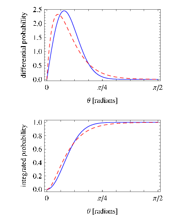
The two distributions are depicted in Fig. 1 for a specific value of $\delta\theta_{i}$. It is worthwhile to note various features of Eqs. (27) and (31):

1. 1.

   When considered as functions of the direction we see that they both depend only $|\hat{n}-\hat{n}_{i}|$ and have a maximum for $\hat{n}=\hat{n}_{i}$, as it should be.

2. 2.

   It is easy to treat them analytically, which is a welcome property to use them in a likelihood.

3. 3.

   It is simple to study their limit for small $\delta n_{i}$ by replacing $\sin\theta\to\theta$ and $\cos\theta\to 1-\theta^{2}/2$, which makes their analytical treatment even simpler.²² 2 When only the second replacement is done, Eq. (27) coincides with the form commonly used in the literature [10] and Eq. (31) practically coincides with the form given in [12]. In fact, the exponential term in Eq. C1 of [12] can be neglected in comparison to the linear term $x$ for all relevant energies.

4. 4.

   For a fixed $\delta\theta_{i}$, we see that $\delta n_{i}$ is smaller in the second case; thus, the maximum at $\cos\theta=0$ is higher in the second case.

5. 5.

   The most probable angle is $\theta\simeq\delta n_{i}$ in both cases; thus it is smaller in the second case.

A choice between Eq. (27) and Eq. (31) (or other reasonable approximations) is not critical for the analysis of SN1987A in view of the limited event sample. However, the use of an appropriate distribution is potentially important for the analysis of the elastic scattering events from a future supernova in a water Čerenkov detector.

We are now in the position to provide a concrete and useful expression for the likelihood that takes into account the reported information on the data and on the detector response.

We recall that:
1) The signal is expected to be uniformly distributed inside the detector. The angular dependence of the signal arises from the angular distribution of positrons produced by $\bar{\nu}_{e}p\to ne^{+}$. This can be expressed as a function of the angle $\hat{n}\hat{n}_{*}$ between the direction $\hat{n}$ of the produced positron and the direction $\hat{n}_{*}$ of the SN1987A. We can thus replace in Eq. (15):

where $V$ is the volume of the detector, the product $\hat{n}\hat{n}_{*}$ can be expressed through Eqs.( 18) and (20) as:

and the factor $2\pi$ accounts for the fact that positron directions are uniformly distributed with respect to rotations around $\hat{n}_{*}$.
2) We assume that the background does not depend on time, direction and position. We indicate the total background counting rate as a function of the energy with $\bar{B}(E)$ and we replace in Eq. (15):

3) The average efficiency of the detector as a function of the energy $\bar{\eta}(E)$ is known. We assume that the efficiency does not depend on time, position and direction, so that we can replace in Eq. (15):

4) The errors on the energy $\delta E_{i}$ and on the direction $\delta\theta_{i}$ in the neighbourhood of the given datum are known. We additionally indicate by $\delta r_{i}$ the value of the error on the position, on which we have only limited information, $\delta r_{i}\sim 1$ m at 10 MeV.

At this point, we have all the elements to write the concrete form of the likelihood. Integrating away the Gaussian on the positions $G_{3}$ and omitting the constant factor $1/(2\pi V)^{N_{\rm ev}}$ we get from Eq. (15):

where Eq. (35) has been rewritten using the intuitive shorthands $\cos\theta\to c$, $\sin\theta_{i}\to s_{i}$, etc.

The first likelihood is Eq. (15) of [4]:

This is an approximation of our likelihood, in that the background has been neglected and the time and angular distribution are integrated (averaged) over; in other words, only the energy distribution is considered. However, this expression is in direct correspondence with Eq. (38), when $B\to 0$ and $\delta\theta_{i}\to 0$, and if we take as the definition of $n(E_{i})$ the one given in Eqs. (18,19,21) of [4]. Furthermore, the expression of [4] agrees with Eq. (2).

The other likelihood that we consider is the one advocated by Lamb and Loredo [5]. This is given by their Eq. (3.18) which, rewritten in our notations, reads

where we neglected dead-time, as appropriate for Kamiokande-II, and dropped the information about the angular distribution. Quoting [5]: Our derivation of the likelihood function reveals errors in previous attempts to account for the energy dependence of the efficiencies of the neutrino detectors; we show that these errors significantly corrupt previous inferences. Indeed, the likelihood advocated by LL has been shown to have an important impact for the analysis of data also by similar and independent analyses of SN1987A observations [13].

We would like, however, to draw the discussion on the correctness of the likelihood of LL. We see that the LL expression, Eq. (40), coincides with our Eq. (38) only if we identify the function $\mathcal{L}_{i}$ with the energy response function of the detector:

where $G_{1}$ is the Gaussian smearing of Eq. (23).

This is not the case for LL who instead claim (see their Eq. (3.21)):

where $E_{0}$ is assumed to be the maximum energy where the efficiency vanishes (i.e., the minimum detectable energy) and $\Theta$ is the step function.

The only special case in which the LL likelihood coincides with our result is when the average efficiency is assumed to be a step function $\bar{\eta}(E)=\Theta(E-E_{0})$. In general, this is not the case and the efficiency is a continuously growing function of the energy. The LL likelihood therefore incorrectly biases the analysis in favor of low energy events. The quantitative effect of this bias on data analysis will be discussed further in Sect. IV.5.

The above remarks amount to the consideration that the likelihood of Lamb and Loredo does not follow from the formal construction described in Sects. II and III. However, it is instructive to point out more directly the profound principle problem of the LL likelihood.

We begin noting that Eq. (40) has been derived by omitting constant terms from

which should represents the probability that a given experimental result is obtained. This expression is supposed to have a general validity. Then consider a simple limiting case: only one bin, with dimension $\Delta t\times\Delta E$ and with energy above $E_{0}$; no background, $B(E)\equiv 0$; a constant signal, $S(E,t)\equiv S$; a constant efficiency, $\overline{\eta}(E)\equiv\eta$; a perfect energy resolution, $\delta E_{i}\rightarrow 0$; a very small expected number of events, $n\equiv\eta S\Delta t\Delta E\ll 1$. In these assumptions, the most probable outcome is the case $N_{\rm ev}=0$, followed by the case $N_{\rm ev}=1$; the probability of other possible results is negligible. From Eq. (43), we calculate the probabilites of the cases when no event and one event are observed: $\mathcal{P}^{LL}_{0}=1-n$ and $\mathcal{P}^{LL}_{1}=n/\eta$ respectively. Their sum violates the basic principle according to which the sum of the probability for all possible results should be equal to one.

We comment here on a likelihood that was not proposed for the analysis of supernova neutrinos, but that it is strictly connected with the previous one.

The same position as in Eq. (42) was made in [14], where Loredo defines the quantity $\ell_{i}(m)=p(d_{i}|m)$. This quantity, that evidently corresponds to the quantity $\mathcal{L}_{i}$ discussed above, is claimed to be independent on the detection efficiency. This position caused the criticism of Loredo [14] to the likelihood advocated for the analysis of trans-neptunian objects of Bernstein et al. 2004 [15] (see Eq. (A8) of [15]). Again, we find the position of [14] unjustified, while we agree with [15]. In particular, Eq. (A4) of [15] expresses the statement that the response function does contain the detection efficiency; it corresponds strictly to our Eq. (4).

Finally, in the analyses performed by some of us [13], Eq. (38) was used, simplified to the case $\delta n_{i}\to 0$ to take into account the mild angular dependence of the $\bar{\nu}_{e}p\to ne^{+}$ reaction. This simplification does not affect significantly the analysis of SN1987A events.

The bias implied by the likelihood of ref. [5] is numerically important already for the analysis of SN1987A events, as found in [5] and confirmed by [13].

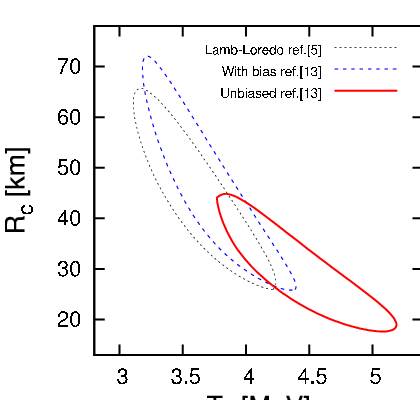
In order to illustrate this point better, we recall certain results obtained in the previous analyses. Let us begin by considering the conventional exponential cooling model, in which the $\bar{\nu}_{e}$ temperature decreases exponentially with the time and the neutrino-radius $R_{c}$ is constant. As evident from Fig. 2, the use of Eq. (42) rather than Eq. (41) leads to important differences on the inferred values of the parameters. We note in particular that the (well-known) difference between $R_{c}$ and the expected size of the neutron star radius, $R_{\mbox{\tiny ns}}\sim 15$ km, is amplified when we adopt Eq. (42) (i.e., when we bias the analysis). This outcome can be easily understood: the bias in favor of low energy events implies that $T_{c}$ (that is proportional to the average energy of the electron antineutrinos) will decrease; thus, $R_{c}$ has to increase to keep the number of events constant.

The bias will be even more important for the analysis of a future galactic supernova, since the number of collected events will be much larger and the errors on the parameters are expected to scale as the square root of the number of the events.

Indeed, the analysis of the 29 events collected by Kamiokande-II, IMB and Baksan in an extension of the exponential cooling model leads to $R_{c}=16^{+9}_{-5}$ km and $T_{c}=4.6^{+0.7}_{-0.6}$ MeV [13]. A recent analysis of simulated events from a future supernova, that assumed the same antineutrino emission model (that includes an initial phase of intense emission), the same central values as found from SN1987A (in particular, $R_{c}=16$ km and $T_{c}=4.6$ MeV), and a supernova located at a distance of 20 kpc (i.e., a data set 30 times larger), leads to the conclusions that the parameters are correctly reconstructed when we use Eq. (41). Moreover, when we combine the results of the simulations, we can estimate the average values of the parameters and of their expected errors: $R_{c}=15.4\pm 0.9$ km and $T_{c}=4.6\pm 0.1$ MeV [16].

The comparison with the values from SN1987A reveals that the errors are expected to decrease by about six times, which is similar to the improvement that we can ascribe to the increased number of data. We are lead to the conclusion that, after a future galactic supernova, the allowed regions in Fig. 2 should shrink by a similar factor in linear scale, making the effect of the bias much more important.

References

- [1] R.M. Bionta et al. Phys. Rev. Lett. 58 (1987) 1494 and C.B. Bratton et al., Phys. Rev. D 37 (1988) 3361; K. Hirata et al., Phys. Rev. Lett. 58 (1987) 1490; K.S. Hirata et al., Phys. Rev. D 38 (1988) 448; E.N. Alekseev, L.N. Alekseeva, I.V. Krivosheina and V.I. Volchenko, Phys.Lett.B 205 (1988) 209.
- [2] D.N. Spergel, T. Piran, A. Loeb, J. Goodman and J.N. Bahcall, Science 237 (1987) 1471.
- [3] T.J. Loredo, D.Q. Lamb, Annals N. Y. Acad. Sci. 571 (1989) 601.
- [4] B. Jegerlehner, F. Neubig and G. Raffelt, Phys. Rev. D 54, 1194 (1996).
- [5] T.J. Loredo and D.Q. Lamb, Phys. Rev. D 65 (2002) 063002.
- [6] Summary table on “ mass” of Particle Data Group: S. Eidelman et al. Phys. Lett. B 592 (2004), page 439; W.M. Yao et al., J. Phys. G 33 (2006), page 472; C. Amsler et al., Phys. Lett. B 667 (2008), page 517.
- [7] A. Strumia and F. Vissani, JHEP 0111 (2001) 048.
- [8] B.T. Cleveland, Nucl. Instrum. Meth. 214 (1983) 451.
- [9] P.J. Kernan, L.M. Krauss, Nucl. Phys. B 437 (1995) 243.
- [10] D. Kielczewska, Phys. Rev. D 41, 2967 (1990).
- [11] M. Nakahata et al., Nucl. Instr. Meth. A421 (1999) 113.
- [12] R. Tomas, D. Semikoz, G.G. Raffelt, M. Kachelriess and A.S. Dighe, Phys. Rev. D 68 (2003) 093013.
- [13] G. Pagliaroli, F. Vissani, M.L. Costantini and A. Ianni, Astropart. Phys. 31 (2009) 163.
- [14] T.J. Loredo, AIP Conf. Proc. 735 (2004) 195.
- [15] G.M. Bernstein et al., Astronomical J. 128 (2004) 1364.
- [16] G. Pagliaroli, F. Vissani, E. Coccia and W. Fulgione, arXiv:0903.1191 [hep-ph], accepted for publication in PRL.