SIGNATURES OF SINGLET NEUTRINOS IN LARGE EXTRA DIMENSIONS AT THE LHC
Abstract
It is a challenge to explain why neutrinos are so light compared to other leptons. Small neutrino masses can be explained if right-handed fermions propagate in large extra dimensions. Fermions propagating in the bulk would have implications on Higgs boson decays. If the Higgs boson is discovered at the Large Hadron Collider (LHC), a detailed analysis may reveal the presence of large extra dimensions. This paper reviews the status of large extra-dimensional models in the context of the current limits on Higgs boson masses and the fundamental Planck scale in extra dimensions.
keywords
neutrinos; extra dimensions; beyond Standard Model1 Introduction
Neutrino oscillation experiments suggest that neutrinos have a very small but nonzero mass.[1]-[11] To explain why neutrinos are so light compared to other leptons is a challenge. The traditional approach is to give neutrinos small mass via a seesaw mechanism. In the type-I seesaw approach, a large right-handed Majorana mass suppresses one of the eigenvalues of the neutrino mass matrix. This leads to a neutrino mass , where is the mass of a light Dirac fermion. The neutrino mixing required to explain the atmospheric, solar, and accelerator neutrino oscillation data requires a super-heavy energy scale for . Explaining the neutrino masses and oscillations is one of the grand challenges of particle physics.
Another interesting challenge is to explain the hierarchy problem: the fine tuning required to maintain a low electroweak scale in the presence of the Planck scale. Supersymmetry, technicolour, and extra dimensions have all been used to address the hierarchy problem. In particular, the extra-dimensions paradigm can lead to the possibility of low-scale gravity.[12]-[14] In the large extra-dimensions approach (often referred to as ADD), the Standard Model (SM) fields are usually localised on (3+1)-dimensional wall (a 3-brane), while gravity is allowed to propagate in all of the dimensions (the bulk). If the fundamental gravity scale is about a TeV, the ultraviolet cut-off for quantum corrections to the Higgs boson mass is also about a TeV. This recasts the hierarchy problem in terms of geometry and the stabilisation of large extra dimensions.
In the large extra-dimensions paradigm, small neutrino masses can be generated without implementing a super-heavy energy scale, as done in a seesaw mechanism11 1 Higher-dimensional seesaw mechanisms are also possible.[15]. Small neutrino masses are naturally explained if at least one right-handed fermion propagates in the extra dimensions.[15]-[17] Since the SM gauge fields are localised to the 3-brane, a bulk fermion must be a SM singlet: “bulk right-handed neutrino” or “singlet right-handed neutrino”. Right-handed neutrinos can freely propagate in the extra dimensions because they have no quantum numbers to constrain them to the SM 3-brane. Therefore, they can also be classified as “sterile” neutrinos. The bulk neutrinos couple to the brane-localised SM fields with small Yukawa couplings. The couplings are small because of the large relative volume of the bulk manifold compared to the thin SM 3-brane. However, because of mixing with a large number of Kaluza Klein (KK) states in the bulk, the interaction probability with the SM fields can be enhanced. Thus the effect of bulk neutrinos on, for example, Higgs boson decays can be significant.
This paper is organised as follows. Section 2 considers some of the experimental results from neutrino experiments that we will use. Section 3 reviews the ideas of right-handed neutrinos in large extra dimensions. The neutrino mass and coupling are discussed in subsection 3.1 and subsection 3.2, respectively. Subsection 3.3 presents bulk neutrinos in other spaces and the effect of compactification. Constraints on the size and number of extra dimensions are discussed in subsection 3.4. Section 4 identifies some of the signatures of right-handed neutrinos in large extra dimensions, which could be revealed by experiments at the LHC. First examined are the implications for the lepton decay of a heavy charged Higgs boson in subsection 4.1. Then, the invisible decay mode of a light Higgs boson is explored in subsection 4.2. Finally, section 5 summarises our findings. With the startup of the LHC, such detailed phenomenological reviews are timely and of value.
2 Some Neutrino Oscillation and Mass Results
Nearly all the useful measurements of neutrino properties, that we will be concerned with, come from neutrino flavour oscillation experiments. Neutrino oscillations imply that the neutrinos have mass and that their lepton flavour is mixed. From neutrino oscillation experiments, one can deduce the absolute difference in the square of neutrino masses. It is common to associate measurements from solar neutrino oscillation experiments with and , and measurements from atmospheric neutrino experiments with and , where and are the neutrino physical masses. The LSND results[18] are not considered in this paper. These results have been shown to be incompatible with solar and atmospheric oscillation data in models of bulk neutrinos.[19]
The experimental oscillation measurements lead to the following results, which are summarised by the Particle Data Group.[20] The current values from solar neutrinos are
| (1) |
at the 68% confidence level. The current bounds from atmospheric neutrinos are
| (2) |
at the 90% confidence level. The best fit is eV2. Only a bound is known on the third angle .
The mass-squared differences can be accommodated within the SM of three active neutrino flavours , , and . Since only the absolute difference of the squares of masses has been determined in atmospheric neutrino oscillation experiments, the order of the masses is not known. Possible mass hierarchies are shown in Fig. 1. For the normal and inverted hierarchies, we typically assume .
For the normal and inverted mass hierarchies, the values of , and are assumed to be of the same order of magnitude as the larger of the mass differences. For the normal mass hierarchy, and is usually assumed. This leads to eV and eV. For the inverted mass hierarchy, and is usually assumed. This leads to eV. In the degenerate mass scheme, eV is a common arbitrary choice.
Current cosmological data and some cosmological assumptions suggest that[20]
| (3) |
Here the sum is over neutrino states that were in thermal equilibrium in the early universe. The mass of the heaviest neutrino is bounded by[20]
| (4) |
where the lower bound is because the mass of the heaviest neutrino cannot be lighter than . This suggests that a more reasonable value to choose for the neutrino mass in the degenerate scheme is 0.7 eV.
3 Right-Handed Neutrinos in Large Extra Dimensions
In this section, we review the aspects of neutrinos in large extra dimensions that will be needed to discuss their effects on Higgs bosons. The ansatz of the large extra dimension paradigm is encompassed in the following relationship.
| (5) |
where GeV is the reduced 4-dimensional Planck scale, is the number of additional spatial dimensions, is the fundamental Planck scale of gravity in -spacetime dimensions, and is the volume of the compact extra-dimensional space (where is the size of the th compact dimension). Assuming the volume has the configuration of a torus, . In the simple case where all of the compact extra dimensions have equal radii , . The case of non-equal radii and configurations other than a torus will be discussed in section 3.4.
Throughout this paper, is used as the definition of the fundamental Planck scale linking experimental measurements to the theory. In the literature on bulk neutrinos in large extra dimensions, it is common to use defined by , and consider as the volume in -dimensional space.
Limits on and have been set by direct gravity measurements, experiments at accelerators, and constraints from astrophysics and cosmology. The Eöt-Washington group constrained the size of the largest extra dimension to m at the 95% confidence level.[21] This completely rules out TeV-scale gravity with one large extra dimension. For two large extra dimensions, they obtain m.[20] The sensitivity to three or more extra dimensions of equal size is only weakly constrained by accelerator experiments. For , is greater than 1.2 TeV and for , is greater than 0.94 TeV from the LEP experiments. For , is greater than 0.8 TeV from the Tevatron experiments. The astrophysical and cosmological limits on are high, particularly for two or three extra dimensions. However, they are based on a number of assumptions so the results are only order of magnitude estimates. Thus, we will not consider further astrophysical or cosmological limits. We will often be interested in the quantity . The best limits on based on the numbers above are eV for , eV for , and eV for .
When adding a right-handed neutrino to the paradigm of large extra dimensions, there are two common approaches taken. One approach is to introduce a separate bulk fermion for each flavour of neutrino on the SM brane.[16, 22] This approach extends the concept of flavour into the bulk. A second approach is to introduce only one bulk fermion and give this fermion a flavour-universal coupling to all three SM brane neutrinos.[23, 24] In this approach, flavour is a feature internal to the SM and is restricted to the SM brane. For simplicity of illustration, we will consider a model of three separate bulk neutrinos.
We can view the Lagrangian density as split into separate bulk and SM brane contributions. The action can be written as
| (6) |
where contains the usual SM Lagrangian plus the interaction terms with the bulk fields, while contains the dynamical terms for the bulk fields and the usual Einstein-Hilbert gravity term. The extra -dimensions are represented by the coordinates . Since we will only be considering thin SM branes, we use the delta function to precisely locate the SM fields and connect the fields on the two manifolds. Small spreading from , such as in models of split fermions, have also been considered.[25]
To further simplify things, we will consider a 5-dimensional theory. In addition, a theory of more than one extra dimension approximates to the 5-dimensional theory when one of the extra dimensions is much larger than the sizes of the other dimensions. The generalisation to more than one extra dimension is straight forward except for one non-trivial detail. This is how the higher-dimensional spinor in the bulk couples to the lepton spinor on the 3-brane. For a generalisation of the 6-dimensional case see Ref. [26].
We begin by adding Dirac fermions to the bulk with wave function , where , and 3 is the flavour index. In the 4-dimensional Weyl basis, a 4-component Dirac spinor can be decomposed as
| (7) |
where and are 2-component complex Weyl spinors. The and subscripts explicitly indicate the 4-dimensional Lorentz property. For the next little while, the flavour index is omitted to simplify the notation.
The 5-dimensional coordinates are , where are not compactified and is a single coordinate perpendicular to the brane. The -direction is compactified on a circle of circumference by making the periodic identification . On the 3-brane .
In the Weyl basis, the 5-dimensional Dirac matrices have size and can be written as
| (8) |
where and , and the are the three Pauli matrices.
The free action for bulk fermions is
| (9) |
where
| (10) |
The bulk action in terms of 2-component spinors is
| (11) |
To obtain the 4-dimensional effective theory, it is common to compactify the large (flat) extra dimensions on a torus by making the identification for each dimension. This suggests performing a KK expansion of the form
| (12) |
where is a vector in number space ( can be positive, negative, or zero), are the KK modes, and are a complete set of periodic orthogonal functions over the space that satisfy
| (13) |
The usual choice for that exhibits the wave nature of the wave function is
| (14) |
For higher-dimensional fermion fields, the KK expansion must include a higher-dimensional Weyl spinor. In the simplified 5-dimensional case considered here, the spinor is the same as the usual 4-dimensional Weyl spinor and is contained in . For higher-dimensions, must have a vector structure and the representation of the chirality multiplets is not unique.
Often Eq. (14) is used for the KK expansion and boundary conditions are imposed afterwards. Since the spectra resulting from toroidal compactification is typically not chiral, we will compactify on an orbifold : the quotient space of a -dimensional torus will inversion symmetry. When an extra space dimension is compactified under the group of isometries, it is natural for one of the 2-component Weyl spinors, e.g. , to be taken to be even under the action , while the other spinor is taken to be odd. The left-handed SM neutrino is restricted to a brane localised at the orbifold fixed point , while vanishes at this point. From the 4-dimensional point of view, a higher-dimensional SM singlet fermion can be decomposed into a tower of KK excitations
| (15) | |||||
| (16) |
where are 4-dimensional states: right- and left-handed Weyl spinors. The first term of is the zero mode and is independent of the extra dimensions. The other terms are called KK modes. We point out that does not have a zero mode.
The 4-dimensional effective theory is obtained by substituting Eq. (15) and Eq. (16) into Eq. (11), and integrating out (dimensional reduction) to obtain
| (17) | |||||
We have now generalized beyond a single extra dimension to the higher extra-dimensional case. The vector in number space now has magnitude , where includes only the positive modes, but excludes the zero mode. We observe the usual tower of KK states in which the Dirac masses are . The sum over can in principle go to infinity, leading to an infinite tower of Dirac KK states. However, we take the view that this extra-dimensional effective field theory description is only valid up to a cut-off scale of approximately and therefore truncate the sum such that the highest KK mass is below . The zero mode decouples from the tower of KK states and is exactly massless.
In the effective 4-dimensional theory, the most general invariant expression describing the interaction between brane and bulk fields is
where is a left-handed lepton doublet, is the SM Higgs doublet with hypercharge , and is a dimensionless Yukawa coupling constant. The flavour indices in Eq. (3) have been suppressed. The coupling can be made diagonal in flavour space by applying two unitary transformations (see section 3.1). The lepton doublet and Higgs field lie on the 3-brane, while the massless Dirac fermion propagates in the full extra-dimensional space. The coupling of Eq. (3) breaks the full Poincaré invariance of the theory by picking out the component from the full Dirac spinor . This can be expected since the presence of the wall itself breaks the higher-dimensional Poincaré transformations. The four dimensional theory is still Lorentz invariant.
One of the crucial questions in explaining neutrino masses and oscillations is the violation of lepton number. We assume lepton number is conserved and assign the opposite lepton number to the lepton doublet in Eq. (3). Since we do not include Majorana masses, the action conserves lepton number and only Dirac neutrino masses are possible for the left-handed neutrinos. There have been a number of models that combine the ideas of large extra dimensions with additional ingredients, such as, small Majorana masses for the brane neutrinos.[15]
The KK states do not mix with each other and the left-handed KK states do not interact with the SM fields. However, the KK states do not completely decouple from the system. The lowest-lying active neutrino (SM neutrino ) will mix with the entire tower of states. Thus the KK states can participate in neutrino oscillations, acting effectively as a large number of sterile neutrinos.
After symmetry breaking by the Higgs mechanism,
| (21) |
The Higgs field acquires a vacuum expectation value (VEV) GeV§. The interaction term in the action becomes
| (22) |
where
| (23) |
Thus, we see that the interactions between the bulk fermions and the brane fields generate Dirac mass terms between the brane fields and all the KK modes of the singlet neutrinos via their Yukawa coupling to the Higgs VEV. The Yukawa couplings of the bulk fields are suppressed by the volume of extra dimensions. The last expression in Eq. (23) appears to be independent of the number of extra dimensions; the number of extra dimensions is hidden in the definition of . In terms of known values
| (24) |
and thus small neutrino masses consistent with neutrino flavour oscillation experiments can be obtained.
In summary, active neutrinos in the SM are Weyl particles of left-handed helicity. Due to gauge invariance, they have no bare mass term. However, left-handed neutrinos on the brane couple to the bulk right-handed fermions, and their interaction allows them to aquire a mass. The left-handed bulk fermions do not couple to particles on the brane since their wave function vanishes at , and thus they decouple from the theory.
3.1 Neutrino Mass
Next we examine the mass eigenvalues and eigenstates. For each neutrino flavour, the mass matrix in KK space can be diagonalised independently. Many authors have diagonalised the mass matrix and written down the neutrino mass eigenstates in a variety of different basis. We follow the approach of Cao, Gopalakrishna and Yuan.[27]
By collecting the neutrino mass terms in the Lagrangian and explicity including the neutrino flavour indices and , we obtain
| (25) |
We make the Yukawa coupling diagonal in the flavour space by applying the rotations[22]
| (26) |
where the unitary matrices and are chosen to diagonalise , such that . The unitary matrices and are similarly chosen to diagonalise the charged lepton mass matrix. This choice of matrices has an advantage in that it does not affect the diagonality of the first term in Eq. (25). The charged current interactions now become proportional to the PMNS matrix[28]-[30]
| (27) |
The Dirac spinors can be define via
| (28) |
Also, for each neutrino flavour, the neutrino mass term in the Lagrangian density can be written as
| (29) |
where . In this basis, the mass matrix is
| (30) |
where are the usual chiral projection operators. This mass matrix is infinite dimensional. The mode number is degenerate with degeneracy , and the elements in the mass matrix are block diagonal.
The mass matrix can be diagonalized by two unitary matrices such that , where is the mass eigenvector. We can reintroduce the generation index and the KK index to write the flavour state in terms of the mass eigenstates as
| (31) |
where is the first row of the unitary matrix.
If we treat the off-diagonal terms in the mass matrix as perturbations22 2 The strong coupling limit has also been investigated.[24], then the zeroth-order lightest eigenvalue of the mass matrix is . In the limit
| (32) |
we have, to a good approximation, a Dirac fermion with mass , and additional Dirac fermions with masses . If the neutrino’s mass is less than , the massive KK modes will have little effect on the neutrino mass term and only the zero mode KK state will generate neutrino mass. In higher order, the lowest mass eigenstate gets an admixture of masses from the KK modes . (Note that only the right-handed components of the KK states mix with the SM neutrino). The perturbative limit in Eq. (32) is satisfied when the brane to bulk coupling is small compared to the compactification scale . It is also necessary to satisfy Eq. (32) so that the probability of active neutrinos oscillating into the sterile KK states is small.
Adding the second order correction to the lowest mass eigenvalue gives
| (33) |
where we identify as the physical SM neutrino mass. For convenience, we define and proceed to calculate the correction 33 3 Some authors have defined the same normalisation as .. This is also the normalisation of the wave function of the lowest eigenstate of the mass matrix. For a single extra dimension, and there is no degeneracy in the mass matrix (). For , the states with mass can be degenerate with degeneracy at the th level. For a large number of KK modes (also possible large ), we can replace the sum over modes by an integral. The leading behaviour is given by the surface of a -sphere of radius in number space.[27] Hence,
| (34) |
where and is the usual Euler gamma function. In calculations, we sum the number of KK modes up to some maximum. In this case, the heaviest KK state that could be produced is limited by . We denote to be the radius of the biggest sphere in number space such that . The sum over KK states can be divergent and depends on . One can show (see A) that
| (35) |
The sum over KK modes converges for , is logarithmic divergent for , and is power divergent for .
The correction causes the physical neutrino mass to be bounded from above. The upper bound depends on the characteristics of the higher-dimensional space: and . The physical mass does not have an extrema (besides 0) but asymptotically approaches the maximum value
| (36) |
when . However, values of that are too high violate Eq. (32). The mixing between the lightest neutrino of mass and heavier neutrinos introduces a correction to the physical neutrino mass ,
| (37) |
Since there is some uncertainty in where exactly the divergence (for ) in the sum over KK modes should be cut off, , and thus , is a bit uncertain. However, must satisfy . Only a rigorously formulated theory, such as string theory, could give precise knowledge of the cut-off parameter.
The perturbative condition places constraints on , , and (and due to the cut-off in the summation). Using Eq. (5) we can re-express the condition on in terms of . Since is not physical, we can replace it by a function of by using Eq. (37) or replace it by a function of by use Eq. (23). We discuss the former case next, and then the later case in section 3.3. For one extra dimension and TeV, the neutrino mass must be less than about eV. In the same scenario, to obtain a neutrino mass of 1 eV, TeV. We find this small neutrino mass or large fundamental Planck scale to be unnatural and do not consider one extra dimension. For , satisfying Eq. (32) gives the results shown in Fig. 2. Current lower limits on the fundamental Planck scale are consistent with current upper limits on the neutrino mass for . For two extra dimensions, rather large values for the fundamental Planck scale and low values for the neutrino mass are required to satisfy the perturbative condition. This makes an unlikely choice in this model. A value of the maximum neutrino mass given by the current limits on atmospheric mixing data of about 0.05 eV would require the fundamental Planck scale to be above about 20 TeV, for . In section 3.4, we will discuss a slight modification of the model which relaxes these constraints.

3.2 Neutrino Mixing
We now briefly consider the implications of higher dimensions on neutrino oscillations. The flavour eigenstates are a non-trivial combination of the physical propagating energy eigenstates that cause the flavour eigenstates to oscillate as a function of time. Good fits to the data from oscillation experiments are obtained by considering only three active species of neutrinos. Strong constraints exist on the mixing of an active neutrino species to a sterile neutrino species.
Let be the probability of an active neutrino species oscillating into another active neutrino species after travelling a distance . The state of the neutrino after a time is determined by the Hamiltonian , and given by the time evolution operator . Thus
| (38) |
Using Eq. (31) and allowing the Hamiltonian to act on the energy eigenstate gives
| (39) |
where is the energy eigenvalue of the th KK mode of the th species.
For a neutrino beam with energy and momentum , in the relativistic limit and are the mass eigenvalues. Hence
| (40) |
The elements of the unitary matrix were given in Ref. [27]. Substituting these matrix elements into Eq. (40), summing over , and assuming gives
| (41) |
to second order in . We see that the oscillations consists of the interference of an infinite number of modes with increasing frequency and decreasing amplitudes . In practice, the high frequency modes can be averaged and only a few low frequency oscillations can be observed, depending on the energy resolution of the detector.
The probability for an active neutrino state to oscillate into sterile neutrino states is
| (42) |
We can use the CHOOZ[31] and atmospheric neutrino data along with Eq. (42) to set bounds on . The mass values given in section 2 can be used for each mass hierarchy scheme. We work in a basis in which the charged lepton mass matrix is diagonal. In this case . For simplicity, we take and the mixing for atmospheric neutrinos to be maximal with . These simplifications give
| (43) |
3.3 Neutrino Coupling
Now consider the Higgs interaction term in the action of Eq. (22). The right-handed neutrino does not carry any electroweak quantum numbers and therefore can be produced only through Yukawa interactions. The Higgs boson couples to a tower of KK neutrino states with the same Yukawa coupling (). In general, the production cross sections and decay widths will be suppressed by the small Yukawa coupling (since the neutrino mass is small), but enhanced by the sum over a large number () of KK excitations of bulk fermions.
As mentioned in the previous section, the perturbative condition Eq. (32) can also be expressed in terms of , , and . Equation (23) can be substituted into Eq. (32), and a condition on and can be obtained for a given . For , is required to be close to the GUT scale of GeV or is required to be infinitesimally small. Thus a single extra dimension is not of interest to us. For , TeV, and for , . Both of these conditions should always be satisfied. Thus TeV and will satisfy the perturbative constraint for all . Some cases for specific values are shown in Fig. 3.

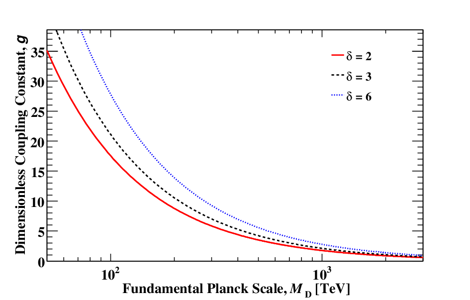
Equations (23), (36), and (37) allow us to relate to the physical neutrino mass , , and . Based on the existing atmospheric neutrino mass best fit of eV, Fig. 4 shows a plot of the dimensionless coupling constant versus fundamental Planck scale. For a perturbative effective theory, can not be arbitrarily large.[32] For , must be about 2000 TeV. This condition has very little dependence on the number of dimensions. If we restrict , the fundamental Planck scale is required to be TeV. Since the UV cut-off scale for the KK sum is somewhat uncertain, is not an unreasonable possibility, but will violate the perturbative constraint for low . Thus, for the model of large extra dimensions that we have just considered, is required to be quite large. Hence we consider small modifications to the model in the next subsection.
3.4 Bulk Fermions in Subspaces and Compactification
A bulk fermion may not necessarily propagate in the same extra-dimensional space that the graviton propagates in. It is possible that the bulk fermion propagates in a subset of the -extra dimensions (). In fact, different bulk fermions could propagate in different dimensions or the UV cut-off scale could be different for each. Thus the formalism for generating small Dirac neutrino masses that we have discussed so far is merely the specific case of . Assuming all the extra dimensions are the same size, the necessary substitutions in the above formula are
| (44) |
The generalisation of Eq. (35) is given in A. In this model, the maximum value of the physical neutrino mass Eq. (36) is given by
| (45) |
for the case of . This is larger than the case. The and 2 cases follow trivially.
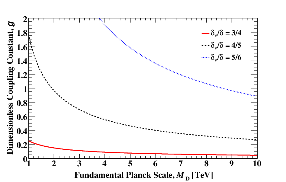
Although is ruled out in the cases of gravity and in the model just presented, is not experimentally constrained. However, for bulk fermions in one dimension, will not be satisfied. Figure 5 shows some cases for a bulk fermion living in a subspace of gravity. TeV is now possible for .
There is no reason for the internal -dimensional manifold to be symmetric. One could imagine compactifying on a product of different dimensional tori , each with its own characteristic radius . The compactification volume would then be , and the mass of the KK states would be
| (46) |
We can create a simplified version of this scenario by adding three assumptions to the theory. These assumptions are that the bulk fermions propagate in a sub-dimensional space of extra dimensions with common size , that gravity propagates in the space of extra dimensions , and that the extra dimensions () have a common size with . With these simplifications Eq. (5) becomes
| (47) |
In this model, the Dirac mass for the SM neutrino Eq. (23) becomes
| (48) |
The volume in Eq. (23) is determined by the compactification scheme. The factor in the denominator is identical if compactified on a torus (circle) or a orbifold. However, more interesting scenarios result in different volumes. For example, for a orbifold the volume becomes .
By including such minor modifications as subspace or alternative compactification schemes to the model, most constraints on the model can be avoided. Throughout this paper we will use “rectangular” toroidal geometry for compactification and express the results in terms of the fundamental Planck scale by using Eq. (5). A pedantic review of the subject would express all results in terms of the compactification volume and leave it to the reader to choose the compactification scheme.
We briefly point out yet another consideration in compactification. Compactification manifolds are not only described by their volume but also by their shape. For example, a general 2-torus is described by three parameters: , , and . Here is a shift angle that is usually taken to be for a “rectangular” torus. The shape parameters of the general 2-torus are and . The physical significance of the angle is that translations along the direction produce simultaneous translations along the direction.[33] Both the volume and shape are important to fully describe the geometry of the compactified extra dimensions. It has been shown that the shape of compactification can dramatically modify the KK spectrum regardless of whether the volume is changed or not.[33]-[35] Thus, the compactification scheme would not only affect the phenomenology of models but also their interpretation if extra dimensions were to be discovered.
3.5 Constraints on the Size and Number of Extra Dimensions
To end this section, we briefly discuss some constrains on models of bulk neutrinos in large extra dimensions. Since gravitons at low energies effect SM processes only marginally, the existence of bulk neutrinos generally impose tighter constrains than those due to gravitational interactions on the scale . In the following, we discuss only a few of the many constraints on bulk neutrinos that have been studied. We refer the reader to the literature for constraints due to anomalous magnetic moments of leptons;[36] nuclear -decay in nuclei;[37] rare charged lepton processes;[38] flavour-violating and universality-breaking phenomena involving and bosons, in addition to leptons;[39] perturbative unitarity violation in Higgs-Higgs scattering;[27] meson and top quark decays through a virtual charged Higgs boson and lepton flavour violating decays through a virtual charged Higgs boson;[40] neutral pion and neutral meson decays to invisible decay modes;[41] and cosmological data.[42]
The luminosity from Supernova 1987a gives strong constraints on extra dimensions.[43, 44] The possible energy loss rate from SN1987a into invisible channels such as the energy carried away by a large number of KK states leads to the following restriction on the size of extra dimensions. The maximum radius of any dimension is keV or Å. The limit is independent of the number of dimensions. For , this constraint requires TeV.
A constraint can also be obtained from big bang nucleosynthesis by the need to avoid too much energy being dissipated into bulk KK neutrino modes before the time of nucleosynthesis. This leads an unacceptable expansion rate of the universe. For , it is likely that too many of the heavy KK modes would be thermal during nucleosynthesis.[16, 17, 43, 45] This would pose a problem for the expansion of the universe.
Intergenerational mass splitting and mixing in large extra dimensions could lead to the violation of lepton universality and flavour changing processes in the charged lepton sector.[46] The mixing of a left-handed neutrino with heavy KK modes alters the tau branching ratio and the decay widths of the charged pion, muon, and tau. Based on experimental limits on lepton universality and flavour changing transitions, is required to greater than about 10 TeV for most of the interesting range of neutrino mass splitting.[46]
There are also constraints on the radius of the extra dimensions resulting from data obtained by oscillation experiments. The data restrict the probability of an active neutrino state to mix into a large number of sterile KK bulk neutrino states. Ref. [22] and Ref. [27] derive the bounds shown in Table 1. Atmospheric neutrino measurements provide the most stringent bounds in the normal mass hierarchy, while CHOOZ[31] data provides the most stringent bounds for the inverted and degenerate mass hierarchies. Ref. [22] uses a model with three active brane neutrinos and three bulk neutrinos. In this case, the results are to be interpreted as constraints on the size of the largest of the extra dimensions, regardless of their total number.
| \topruleExtra Dimensions | Normal | Inverted | Degenerate |
|---|---|---|---|
| \colruleNA | 0.24 | 0.60 | 10.9 |
| \colrule1 | 0.15 | 0.5 | 10.6 |
| 2 | 1.5 | 5.3 | 100 |
| 3 | |||
| \botrule |
Given the above constraints and to avoid problems with standard big bang nucleosynthesis, we require throughout this paper.
4 Collider Signatures
Testing the origin of small neutrino masses at the LHC is a hot and important topic.[47, 48] There are already many papers on how to test a variety of seesaw mechanisms[49] and look for heavy Majorana[50] (or Dirac) neutrinos at the LHC.
If right-handed bulk fermions are responsible for the small mass of a neutrino, what are the consequences at the LHC? Higgs boson production and decay could be measurably altered from SM or supersymmetry (SUSY) expectations. Possible couplings are shown in Figs. 6 and 7. We will use the symbol to represent the set of right-handed KK states, including the right-handed zero mode. Although right-handed bulk neutrinos would couple to all types of Higgs bosons, we restrict our discussion to the SM Higgs boson and a charged doublet of Higgs bosons.
We review the current bounds on the Higgs boson masses.[51] From electroweak fits and a cut-off scale at the 4-dimensional Planck scale, the SM Higgs boson mass is restricted to GeV44 4 The neutral Higgs boson will be denoted by without the neutral charge indicated.. If new physics appears at a lower mass scale of 1 TeV, the bounds becomes weaker: GeV. Since GeV from the LEP experiments, we do not consider SM Higgs boson masses below 100 GeV. The region GeV has also recently been exclude by the Tevatron experiments.[52] For the charged Higgs boson, GeV is allowed from the LEP experiments and the Tevatron experiments can limit for or , where is the top quark mass. We will be interested in charged Higgs bosons that can decay to top quarks and thus limit our considerations to charged Higgs boson masses above 170 GeV.
Bulk fermions are not the easiest particles to detect. The KK states behave as massive, noninteracting, stable particles, and thus appear as missing energy in the detector. The , , and KK states all lead to missing energy, and their detection must be indirect.
4.1 Tau Decay of a Heavy Charged Higgs Boson
In this section, we review the possibility of a heavy charged Higgs boson decaying to a lepton within the model of bulk fermions in large extra dimensions. In typical SUSY models is allowed, while is completely suppressed55 5 In the following, the charged Higgs boson is denoted by , but the is also implicitly included.. Models of bulk fermions in large extra dimensions allow for the possibility of , where is a singlet neutrino.
Many extensions to the SM include a charged Higgs boson. We will consider the two-Higgs doublet model of type II (2HDM-II). In this model, each doublet has a unique hypercharge . The Higgs doublet with couples to right-handed up-type quarks and neutrinos, while the Higgs doublet with couples to right-handed down-type quarks and right-handed charged leptons. An example of such a model is the Minimal Supersymmetric Standard Model (MSSM). In the MSSM there are two vacuum expectation values related by , where is the VEV of the doublet and is the VEV of the doublet. The VEV GeV is given by .
In the framework of large extra dimensions with bulk fermions, there is no need to postulate additional Higgs bosons beyond the two doublets. Thus the charged Higgs boson is produced identically as in the 2HDM-II. For a light charged Higgs boson, the dominant production mechanism is through the decay of the top quark . To focus the discussion, we consider only a heavy charged Higgs boson with mass larger than the top quark mass. We will consider the production process , as shown in Fig. 8. Charged Higgs boson production in association with a top quark is the dominant process and thus we ignore the processes , , , and , where is a light quark.
Figure 9 shows the leading-order cross section for charged Higgs boson production for masses above the top quark mass. The Yukawa and SUSY electroweak corrections have been calculated along with the one-loop SUSY corrections. The complete next-to-leading order (NLO) QCD corrections have been calculated and are significant. The NLO SUSY-QCD corrections are small in comparison. The next-to-next-to-leading order (NNLO) corrections have been calculated near threshold.[53]-[57]

The process is also possible. This and overlap when summing the theoretical contributions. Thus one must be careful to avoid double counting when tagging jets. Alwall and Rathsman[58] have addressed this problem and provided code[59] to handle the proper matching in the Monte Carlo generation of events. Double counting has been avoided in Fig. 9 by using Ref. [59].
Branching ratios versus the mass of the charged Higgs boson for two different values of in the MSSM are shown in Fig. 10. The program HDECAY with default parameters has been used.[60] Above the top quark mass threshold, the decay mode dominates. This mode suffers from a large irreducible background and a large combinatorial background. A fraction of heavy charged Higgs bosons are allowed to decay into other modes, depending on the SUSY parameters. Particularly, the decay modes and can be important. The discovery potential is dominated by , which despite its significantly smaller branching ratio for low , allows more efficient background suppression. For high charged Higgs boson masses, decays to SUSY particles may be kinematically allowed, but we do not consider this possibility. This paper assumes the mass scale of the SUSY partners are above so that the decays of to SUSY particles are forbidden.


In the following, we focus on the process
| (49) |
The charged Higgs boson decay to a lepton is the strongest one affected by the model of bulk fermions in large extra dimensions.[40]
Although both the boson and charged Higgs boson can decay to leptons, there are important differences in their decays. Unlike the boson that couples universally to all three leptons, the charged Higgs boson couples preferentially to the heaviest lepton ( lepton). Since the charged Higgs boson is a scalar particle, the helicities of the final state particles must be different. This is opposite to the decay of the boson, which is a vector particle. Thus, in the MSSM, is allowed but is forbidden (at tree level) since SM neutrinos are left-handed.
For the charged Higgs the corresponding interaction term in the action corresponding to Eq. 22 is
| (50) |
The corresponding couplings are given in B. Thus, in models of large extra dimensions with bulk fermions, both lepton polarizations are allowed: the usual MSSM mode 66 6 For the remainder of this subsection, we drop the subscript on and consider to be either the usual neutrino of the SM or the left-handed neutrino in models of large extra dimensions with bulk fermions. and the new mode , where is the right-handed bulk neutrino. The usual charged Higgs boson decays to leptons through the Yukawa coupling. The SM neutrino is now predominantly a light neutrino plus a small admixture of KK modes with mass of order . Thus this decay is also effected by the presence of the right-handed fermion in the extra dimensions. The decay width is modified relative to the 2HDM-II calculation, , provided (see B):[40]
| (51) |
where
| (52) |
and
| (53) |
In calculating , the KK states have been summed up to , i.e. they are required to be lighter than the charged Higgs boson mass (see C). If , must be replaced by . The quantities in the extra factor partially compensate each other. In the parameter space in which is large, will also be large, and when is small, is small. The factor varies with charged Higgs boson mass but over the range 170 to 600 GeV there is little increase in for low number of extra dimensions. Thus is typically about 0.1 and is always less than unity.
In models of large extra dimensions with bulk fermions, the charged Higgs boson can also decay to a left-handed lepton and a right-handed neutrino. A calculation of this decay width gives (see B)[40]
| (54) |
where
| (55) |
In the calculation of , the lepton mass has been neglected and the right-handed neutrino KK states have again been summed up to the threshold for the decays.
In the MSSM at the tree level there are only two parameters: typically chosen to be the mass of the CP-odd scalar Higgs boson and . In contrast, the parameter space of a model of large extra dimensions with bulk fermions depends on , , , , and . To get a feel for the relative importance of the two helicity modes, the ratio of decay widths of left-handed to right-handed leptons is approximately
| (56) |
where for simplicity the normalisation due to mixing , and the phase space factors and have been ignored. For typical parameter values, . Part of this high value of is because the decay width to is suppressed by a factor of about 10 relative to the 2HDM-II, as discussed previously. The major factor that results in being high is a large multiplicity factor due to the large number of KK states, despite a small Yukawa coupling to and a single KK neutrino. The value of can also be low for high and high .
Figures 11 and 12 show charged Higgs boson branching ratios for models of large extra dimensions with bulk fermions. Three extra dimensions was chosen and a value of TeV was used to ensure the neutrino masses were consistent with the atmospheric neutrino data. Dirac masses of eV (corresponding to eV2) and eV (corresponding to eV2) have been chosen to lie in the allowed experimental range. For small , we see similar decay branching ratios for models of large extra dimensions with bulk fermions as in the MSSM. As gets larger, becomes dominant for small values.


In searching for the effects of bulk neutrinos in charged Higgs boson decay, we need to both extract a signal of charged Higgs boson events above background events, and show that the resulting signal events agree with the large extra dimensions scenario. If one tries to just exploit the lepton polarization difference to separate bulk fermions in large extra dimension models from the MSSM, one is probably not able to reduce the background from SM boson decays, as these have the same signature as our extra dimensional model signal. First, we must reduce the SM background to get a clean sample of charged Higgs boson events. After this, an attempt can be made to use the lepton polarization to determine the charged Higgs boson decay mechanism, and hence, rule out the MSSM or large extra dimensions model.
One of the backgrounds to our production channel of interest is single top quark production , where the boson mimics the charged Higgs boson. The cross section times branching ratio for this background is about 48 pb. Another background is production with one and the other . The cross section times branching ratio for this background is about 84 pb. For the signal, the cross section times branching ratio can be about 0.04 pb to 3.46 pb over the charged Higgs boson mass range of GeV and from 1.5 to 30. The background will need to be reduced by a factor of about 40 to 3000. The above branching ratio times cross section values have been obtained from Ref. [61].
The differences between signal and background have been examined in Refs. [61, 62], and more recently, in Ref. [51]. We largely follow the discussion in Ref. [61]. Since we are interested in the lepton decay modes of the charged Higgs boson, we require a well reconstructed jet. One-prong hadronic decays of the lepton are identified and the reconstructed jet is required to have high transverse momentum to reduce the soft jet backgrounds. The reason we chose single-prong hadronic lepton decays will be explained when we discuss measuring the lepton polarization.
Since the charged Higgs boson is produced in association with a top quark, we reconstruct single top quark events. Typically, at least three non- jets with high would be required. One of these jets, and only one, would need to be tagged as a jet. Two of the non-tagged jets would be required to have an invariant mass close to the boson mass. These two jets would have their energy adjusted to reproduce the boson mass and the resulting energy-rescaled jets would be combined with the jet to reconstruct the three-jet invariant mass. Events with a three-jet invariant mass close to the top quark mass would be selected for further analysis.
The difference in mass between the charged Higgs boson and the boson can also be exploited. The bosons are highly boosted in the laboratory frame of reference and hence the lepton is approximately collinear with the neutrino along the direction of the original boson. Thus the distribution of the azimuthal opening angle between the jet and the missing transverse energy77 7 Although we call this quantity missing transverse energy, we really mean the negative of the vector sum of all the visible transverse momenta in the event. should be peaked at small values for boson decays. The azimuthal angle should be larger for leptons from charged Higgs boson decays.
The difference in mass between the charged Higgs boson and the boson can be exploited further. Because of the neutrino in the final state, only the transverse mass can be reconstructed:
| (57) |
In background events, the transverse mass has an upper bound at the boson mass, while in the signal events it is constrained by the charged Higgs boson mass. However, due to finite resolution (particularly on ), there is leakage of the background into the signal region. To optimise the signal to background ratio, a requirement is imposed on the transverse mass ( GeV, for example). In addition, a cut on (, for example) can be applied. Using such a set of requirements as described above and a simple simulation of the ATLAS detector, Assamagan and Deandrea[61] have shown that a significance (defined by ) greater than five can be obtained with 100 pb-1 of data. Using a detailed simulation of the ATLAS detector, the charged Higgs boson should be detectable in a significant faction of the (, ) parameter space with the first 10 fb-1 of data.[51] The discovery reach is most likely limited by the signal size itself.[61]
Observation of a signal in the transverse mass and azimuthal opening angle distributions could help one to obtain a clean sample of charged Higgs boson events. Unfortunately, this would not allow one to determine weather the scenario is the MSSM or not. A further measurement of the polarization asymmetry might provide distinctive evidence for models with bulk fermions in large extra dimensions. We can look at the lepton polarization asymmetry which is defined as
| (58) |
In the 2HDM-II, is . In the model of bulk fermions in large extra dimensions, is also allowed but would have a different phase space since the neutrino contains an admixture of KK modes. For small values of the lepton is right-handed (expect for small values of ). Left-handed leptons are produced for large .
To study the lepton polarization, consider the hadronic single-prong decays
| (59) |
These decays best imprint the information of the polarization onto the decay products. Experimentally, one does not distinguish between and mesons, and and mesons. Thus a small contribution from the kaon modes is present. The above decays correspond to about 90% of the hadronic one-prong decays and thus should represent the lepton polarization effects. We make the approximation that the decay products of the lepton merge along the lepton line of flight in the laboratory frame (collinear approximation).
To take advantage of the direction of the charged meson encoding the lepton information, the momentum of the meson relative to the energy of the jet , , could be examined. The ratio is related to the angle that measures the direction of the charged hadron in the lepton rest frame relative to the lepton line of fight, which defines its polarization axis.[63] In the case of MSSM, the mesons coming from charged Higgs boson decays are peaked at . The distribution is peaked at and for longitudinal and mesons, but is in the middle for transverse and mesons. In the case of models with bulk fermions or background due to decay, the contributions to the distribution are reversed; the mesons coming from the boson decays are peaked at . Since it is anticipated that the discover reach is limited by the signal size itself, the backgrounds, after the above reduction, are expected to be very small. Thus the distribution could be examined to reveal the model for charged Higgs boson decays. The distribution should be peaked at and for the MSSM. For models of bulk fermions in large extra dimensions, the distribution would depend on the polarization asymmetry. In the case of a polarization asymmetry of about one (about 100% left-handed leptons) the distribution would be peaked near the centre.
In summary, although one could claim a discovery by observing a charged Higgs boson, it would be insufficient to say what beyond the SM physics produced it. Further measurement of the polarization asymmetry might provide distinctive evidence for the model of bulk fermions in large extra dimensions.
4.2 Invisible Decay of a Light Higgs Boson
Higgs boson invisible decays have been discussed in a number of models for physics beyond the SM.[64] To trigger on the invisible decay mode of the Higgs boson, the Higgs boson must be produced in association with other particles. In addition, one can not reconstruct the Higgs boson directly but must probe the signal indirectly through the missing energy distribution.
For invisible Higgs boson decay in models of bulk neutrinos, no additional production mechanisms beyond the SM are necessary. The cross sections for SM Higgs boson production are shown in Fig. 13. The gluon-gluon fusion channel, via a top quark loop, is dominant. However, since there is nothing else in the event besides the Higgs boson, this channel is of little use for triggering on Higgs boson invisible decays. The vector-boson vector-boson fusion process () has recently been shown to be a viable channel for triggering and searching for Higgs boson invisible decays.[51] Because of its large cross section, it has become a channel of interest. The jets are preferentially separated in rapidity and are correlated in azimuthal angle. A low-luminosity trigger, which triggers on missing transverse energy plus a forward jet plus a cental jet is possible. At higher luminosity there will be more activity in the rapidity gap and it is not known how effective the trigger will be. Further discussion of this channel is beyond the scope of this phenomenological review. Other useful channels are the Higgs-strahlung processes (), or associated production with a vector boson, and associated production with a top quark. Associated production with a top quark has not received much attention and it is anticipated to be less useful then the Higgs-strahlung processes.

Associated production with the boson occurs via , which is followed by and invisible. The composite signature to be observed from this decay is 1) no hadronic activity, 2) missing transverse momentum, and 3) a high- lepton. Background due to off-shell production and its leptonic decay overwhelm the signal channel by a factor of more than 200 even after background rejection cuts.[65] We will examine this process in more detail in the next subsection.
A better channel is associated production with the boson
| (60) |
where ( or only) and invisible. The lepton decay mode of the boson is usually not considered because of uncertainties in lepton identification and the resulting poor invariant mass resolution from using leptons to reconstruct bosons. The signature from the decay is 1) no hadronic activity, 2) missing transverse momentum, and 3) two high- same flavour charged leptons with invariant mass close to the mass of the boson. The two high- leptons trigger the event.
There is an irreducible background to the process in Eq. (60) from production, where one boson decays leptonically and the other boson decays into neutrinos. Since is produced by -channel processes, it is expected that the distribution of the bosons will be softer than the distribution of the bosons from the -channel production process. The next most significant irreducible background is from production with each decaying leptonically. This background has a considerably softer transverse momentum distribution. Since both of these backgrounds have softer transverse momentum distributions than the signal, to may be possible to detect a signal by requiring high missing transverse energy. Other backgrounds arise from , , and , but they can be suppressed.
The decay channel must also be consider in the process in Eq. (60). The advantage of this channel is the increased branching fraction of compared to . The disadvantages are the lower efficiency for identifying final states compared to leptonic final states, the reduced boson invariant mass resolution, and the more difficult background sources. These backgrounds include contributions from , , , , single top quark, and production. The significance of the channel is not as high as in the lepton channel, but this channel could be combined with the lepton channel, or be used to confirm an observed signal. Another potential background to the process in Eq. (60) is and .
The SM Higgs boson can decay to plus a right-handed bulk neutrino in models of large extra dimensions. The invisible decay width summed over all neutrino flavours is (see B)[17, 41, 64]
| (61) |
The Higgs boson decay to the final state is proportional to which is extremely small. However, the multiplicity of KK states below is , which can be very large. It is proportional to the volume of the -dimensional space times a momentum-space factor of order .
Figure 14 shows the Higgs boson branching ratios versus Higgs boson mass for SM processes and a model with bulk fermions in large extra dimensions. Below a Higgs boson mass of 135 GeV the decay mode dominates, while above 150 GeV the decay mode dominates.


Since dominates at low Higgs boson masses, it is useful to consider the ratio
| (62) |
Figure 15 shows the ratio in Eq. (62) versus fundamental Planck scale. The invisible decay mode of the Higgs boson is significant for and low . For TeV, the invisible decay width of the Higgs boson will be negligibly small compared to . One way to reduce is to consider a bulk fermion propagating in a subspace of the full extra dimensions (see section 3.4). With and , can now be as low as a TeV. Only in a very small region of parameter space can the invisible decay of the Higgs boson be as large as the decay mode. The main restriction comes from the perturbative constraint on the Yukawa coupling . Asymmetric dimensions also allow us to reduce while keeping .

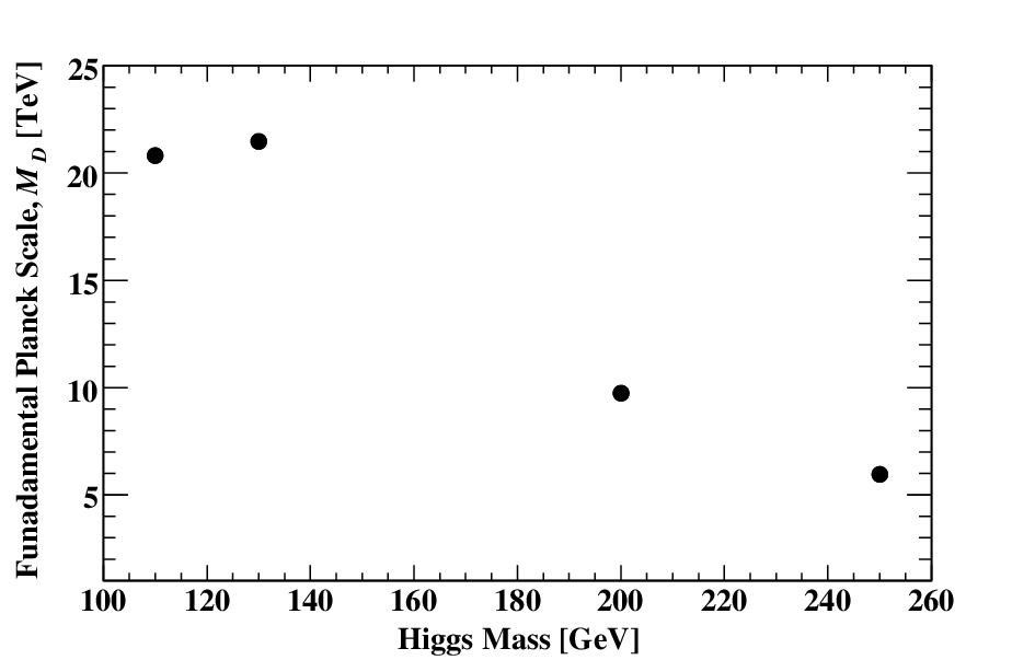
Recently, the ATLAS collaboration has performed a detailed study of its detector’s sensitivity to an invisibly decaying Higgs boson.[51] Model independent limits were set on the branching ratio time cross section divided by the SM Higgs boson cross section. Assuming the SM Higgs boson production cross section for models of bulk fermions, limits can be set on the invisibly decay branching ratio as a function of the neutrino mass, fundamental Planck scale, and the number of extra dimensions. For three extra dimensions and a bulk Dirac fermion mass eV, lower limits can be set on the fundamental Planck scale. Figure 16 show the derived lower limits on the fundamental Planck scale using the vector boson fusion limits in Ref. [51].
In summary, in certain regions of extra-dimensional parameter space, the branching ratio of Higgs boson decay into invisible modes can be greater than , but the Yukawa coupling is large. For reasonable values of , the invisible decay rate is a tiny fraction of the rate.
4.2.1 Associated Production of Bulk Neutrino with Light Higgs Boson
We now discuss in more detail the process of off-shell production and its leptonic decay. Consider the process (Fig. 17)
| (63) |
where is a KK mass eigenstate. The process is mediated by .
In calculating the cross section, we again work in a basis in which the charged lepton mass matrix is diagonal and is given by Eq. (43). Cao, Gopalakrishna, and Yuan[68] have shown that it is also beneficial to work in a bases in which is rotated with matrix , since this absorbs the unphysical matrix into the definition of . It was also found that one should retain in the flavour basis in order to explicitly keep only the physical matrix . In this basis, the total production rate for process in Eq. (63), summed over all lepton flavours, is proportional to , where , and is a physical diagonalised neutrino mass matrix. Using the neutrino data in section 2, the matrix in each mass hierarchy scheme is
| (64) |
| (65) |
| (66) |
and the values are (0.0509 eV)2 for the normal, (0.0707 eV)2 for the inverted, and (1.732 eV)2 for the degenerate mass hierarchy schemes.
The cross section summed over all lepton flavours , and as a function of , , , and has be calculated in Ref. [68]. The cross section is less than a femtobarn for , so we will focus on . The cross section decreases slightly with increasing Higgs boson mass. However, the main dependence is on (or ) with fb for TeV. Besides the new physics production mode, there is also the previously discussed production mode , which has been show to be indistinguishable from SM background processes.[65]
The Higgs boson can decay to the usual SM decay modes, as well as the invisible decay mode that we have described previously. The SM modes and are dominant. Since the invisible decay mode can only dominate at low Higgs boson masses GeV, we restrict our attention to this mass region and will not consider the decay mode. It should also be noted that it is difficult to detect the state. This is because the leptonic decay branching ratio is suppressed and the hadronic decay modes are dominated by background.
We consider the two Higgs boson decay modes, invisible and , for the new process. The decay mode
| (67) |
suffers from large background. However, this channel allows the invariant mass of the Higgs boson to be reconstructed. The signature is plus missing energy, where we will only consider or , because of the difficulty in reconstructing the different decay modes of the jet. We will assume the jets can be tagged by an experiment with an efficiency of about 50%, say. Two intrinsic SM processes dominate the background
| (68) | |||||
| (69) |
Ref. [68] has shown, that even with a perfect detector, for , TeV, GeV, and 100 fb-1 of data, only eight events above a background of can be obtained. Therefore it would be extremely difficult to use the mode to directly detect the signal at the LHC. However, a novel approach employing state-of-the-art jet reconstruction and decomposition techniques indicates that is a promising search channel for a SM Higgs bosons around 120 GeV in mass.[66] A recent study by the ATLAS collaboration has confirmed the viability of the new technique.[67]
Now consider the decay mode
| (70) |
The signature is , or plus missing energy. For the , we will consider only the decay mode. So the resulting signatures are plus missing energy or plus missing energy, where now or only. The major SM background is the Drell-Yan charged current process .
To search for an invisible decay mode, one can apply a set of cuts to enhance the signal to background and then look at the shape of the missing transverse energy spectrum. The procedure must be applied to the different mass hierarchy schemes separately since the relative numbers of each lepton type in the final state differ. Ref. [68] has shown that the and channels lead to similar significances. If is about 5 TeV (for normal or inverted) or about 20 TeV (for degenerate) we may expect the significance to be in the range of .[68] If we strictly impose the constraints on , we would expect a poor significance. However, we have pointed out previously that because of the dependence on the UV cut-off for , those constraints are uncertain to some extend. Therefore, in the event that the constraint on is relaxed somewhat, we may expect to see a signal at the LHC. We may also expect to see a signal if we consider a model with bulk neutrinos in a subspace of extra dimensions, or asymmetric dimensions.
Neutrino oscillation data do not give the sign of nor the absolute scale of the neutrino masses. Measuring the sign of would determine directly whether the normal or the inverted mass hierarchy is realized in nature. Can we use the collider observables to distinguish between the normal, inverted, or degenerate mass schemes? We can define a lepton flavour asymmetry. Let and be the number of electron and muon signal events, respectively. Define
| (71) |
From this asymmetry one can obtain
| (72) |
where the upper sign is for the normal mass hierarchy and the lower sign is for the inverted mass hierarchy. Thus for the normal mass hierarchy and for the inverted mass hierarchy. For the inverted mass hierarchy, the smallest value that can take is 0.05 eV. Figure 18 shows the ideal situation with no experimental affects included. For small , there is excellent discrimination power to determine whether the normal or inverted mass hierarchy is realized. However, as is increased, the number of , and lepton events becomes approximately equal and the discriminating power diminishes. We might also be able to determine the absolute scale of the neutrino mass , but only if is not too large compared to . The (or ) asymmetry does not add any additional information in probing the neutrino masses.

In summary, a signal of significance for and TeV (normal or inverted mass hierarchies), or TeV (degenerate mass scheme) could be obtained.[68] If a positive signal is found, the asymmetry in muon versus electron events could distinguish between the neutrino mass hierarchies and determine the absolute neutrino mass scale. The LHC might be a unique place to determine the hierarchy and mass scale as it is not available from neutrino oscillation experiments.
5 Summary
Singlet fermions in the bulk couple to the SM states on the brane as right-handed neutrinos with small couplings. The Yukawa couplings of the bulk fields are suppressed by the large volume of the extra dimensions. The interaction between the bulk fields and the brane fields generate Dirac mass terms between the neutrinos and all the KK modes of the bulk fields.
The effects of bulk neutrinos could be observed in charged Higgs boson decays. A clean sample of charged Higgs bosons would be needed to identify the model in which they are realized.
Observation of Higgs boson invisible decays in models of large extra dimensions could provide an opportunity to distinguish between the normal and inverted neutrino mass hierarchies, and to determine the absolute scale of the neutrino masses. Doing this requires measuring the asymmetry of the observed event numbers in the electrons and muons produced in association with the Higgs boson.
Observation of Higgs bosons in models with large extra dimensions will be difficult. This is due to the need to keep the dimensionless coupling constant low enough so that the effective theory is perturbative. However, models of asymmetric dimensions or bulk fermions living in a subspace of the extra dimensions allow a good chance to observe Higgs bosons at the LHC.
Acknowledgments
This work was supported in part by the Natural Sciences and Engineering Research Council of Canada.
Appendix A Mass Mixing Normalisation Factor
In this appendix, we perform the sum over KK states in the normalisation factor of the mass mixing. From Eq. (33),
| (73) |
We have dropped the “hat” notation in the last expression. For generality, we will not require the number of extra dimensions that the bulk fermion propagates in to be the same as the number of extra dimensions of gravity . To obtain expressions for the case when the two spaces are the same take .
For , the sum can be evaluated directly and the upper bound on the sum can be taken to infinity.
| (74) | |||||
where Eq. (5) has been used to replace in terms of and in the second expression.
For , the infinite sum does not converge so we replace the sum by an integral over a sphere.
| (75) |
where . We have
| (76) |
For ,
| (77) | |||||
For ,
| (78) | |||||
In the first line of above expression, we have made the approximation that the lower bound of integration can be taken to be zero.
Appendix B Scalar Boson to Two-Fermion Decay Widths
The decay width is
| (79) |
where the magnitude of either outgoing momentum in the boson rest frame is
| (80) |
If or (),
| (81) |
If and ,
| (82) |
The matrix element consists of a vertex factor times a spinor product
| (83) |
The spinor product for a signal polarization state is
| (84) |
If ,
| (85) |
If and ,
| (86) |
For fermions (not neutrinos), there will be two polarization states and hence the matrix element squared should be multiplied by a factor of two. For SM neutrinos this factor of two will be absent. Including the two polarization states, we have
| (87) |
for .
| (88) |
for and .
B.1 SM Higgs Boson and MSSM Charged Higgs Boson Decay Widths
For the SM Higgs boson,
| (89) |
For in MSSM,
| (90) |
For in MSSM,
| (91) |
Consider in MSSM. Using , , and gives
| (92) |
B.2 Large Extra Dimensions Decay Widths
Consider in the model of bulk fermions in large extra dimensions. We separate the zero mode from the modes; . Using , , , and , gives
| (93) | |||||
See C for a calculation of .
Consider . Using , , and gives
| (94) | |||||
See C for a calculation of .
Appendix C Kaluza Klein Phase Space Sums
For bulk fermions, the masses of the KK states are not negligible, nor are the masses of the final two particles equal. Thus with summed over the number of KK states is the quantity of interest in the decay width.
| (95) | |||||
Also of interest is
| (96) | |||||
References
- [1] Y. Fukuda et al., Phys. Rev. Lett. 81, 1562 (1998).
- [2] Y. Fukuda et al., Phys. Rev. Lett. 86, 5651 (2001).
- [3] Q.R. Ahmed et al., Phys. Rev. Lett. 87, 071301 (2001).
- [4] Q.R. Ahmed et al., Phys. Rev. Lett. 89, 011301 (2002).
- [5] Q.R. Ahmed et al., Phys. Rev. Lett. 89, 011302 (2002).
- [6] K. Eguchi et al., Phys. Rev. Lett. 90, 021802 (2003).
- [7] S.N. Ahmed et al., Phys. Rev. Lett. 92, 181301 (2004).
- [8] Y. Ashie et al., Phys. Rev. Lett. 93, 101801 (2004).
- [9] T. Araki et al., Phys. Rev. Lett. 94, 081801 (2005).
- [10] Y. Ashie et al., Phys. Rev. D 71, 112005 (2005).
- [11] B. Aharmim et al., Phys. Rev. C 72, 055502 (2005).
- [12] N. Arkani-Hamed, S. Dimopoulos and G. Dvali, Phys. Lett. B 429, 263 (1998).
- [13] I. Antoniadis, N. Arkani-Hamed, S. Dimopoulos and G. Dvali, Phys. Lett. B 436, 257 (1998).
- [14] N. Arkani-Hamed, S. Dimopoulos and G. Dvali, Phys. Rev. D 59, 086004 (1999).
- [15] K.R. Dienes, E. Dudas and T. Gherghetta, Nucl. Phys. B 557, 25 (1999).
- [16] G. Dvali and A.Y. Smirnov, Nucl. Phys. B 563, 63 (1999).
- [17] N. Arkani-Hamed, S. Dimopoulos, G. Dvali and J. March-Russell, Phys. Rev. D 65, 024032 (2001).
- [18] A. Aguilar et al., Phys. Rev. D 64, 112007 (2001).
- [19] R.N. Mohapatra and A. Pérez-Lorenzana, Nucl. Phys. B 593, 451 (2001).
- [20] C. Amsler et al., Phys. Lett. B 667 (2008).
- [21] D.J. Kapner, T.S. Cook, E.G. Adelberger, J.H. Gundlach, B.R. Heckel, C.D. Hoyle and H.E. Swanson, Phys. Rev. Lett. 98, 021101 (2007).
- [22] H. Davoudiasl, P. Langacker and M. Perelstein, Phys. Rev. D 65, 105015 (2002).
- [23] K.R. Dienes and I. Sarcevic, Phys. Lett. B 500, 133 (2001).
- [24] C.S. Lam and J.N. Ng, Phys. Rev. D 64, 113006 (2001).
- [25] K.R. Dienes and S. Hossenfelder, Phys. Rev. D 74, 065013 (2006).
- [26] J. Matias and C.P. Burgess, J. High Energy Phys. 0509, 052 (2005).
- [27] Q.-H. Cao, S. Gopalakrishna and C.-P. Yuan, Phys. Rev. D 69, 115003 (2004).
- [28] B. Pontecorvo, JETP 7, 172 (1958).
- [29] B. Pontecorvo, JETP 26, 984 (1968).
- [30] Z. Maki, M. Nakagawa and S. Sakata, Prog. Theor. Phys. 28, 870 (1962).
- [31] M. Apollonio et al., Phys. Lett. B 466, 415 (1999).
- [32] K. Agashe and G.-H. Wu, Phys. Lett. B 498, 230 (2001).
- [33] K.R. Dienes, Phys. Rev. Lett. 88, 011601 (2002).
- [34] K.R. Dienes and A. Mafi, Phys. Rev. Lett. 88, 111602 (2002).
- [35] K.R. Dienes and A. Mafi, Phys. Rev. Lett. 89, 171602 (2002).
- [36] G.C. McLaughlin and J.N. Ng, Phys. Lett. B 493, 88 (2000).
- [37] G.C. McLaughlin and J.N. Ng, Phys. Rev. D 63, 053002 (2001).
- [38] A. de Gouvêa, G.F. Giudice, A. Strumia and K. Tobe, Nucl. Phys. B 623, 395 (2002).
- [39] A. Ioannisian and A. Pilaftsis, Phys. Rev. D 62, 066001 (2000).
- [40] K. Agashe, N.G. Deshpande and G.-H. Wu, Phys. Lett. B 489, 367 (2000).
- [41] N.G. Deshpande and D.K. Ghosh, Phys. Lett. B 567, 235 (2003).
- [42] K.N. Abazajian, G.M. Fuller and M. Patel, Phys. Rev. Lett. 90, 061301 (2003).
- [43] R. Barbieri, P. Creminelli and A. Strumia, Nucl. Phys. B 585, 28 (2000).
- [44] G. Cacciapaglia, M. Cirelli and A. Romanino, Phys. Rev. D 68, 033013 (2003).
- [45] H.S. Goh and R.N. Mohapatra, Phys. Rev. D 65, 085018 (2002).
- [46] A.E. Faraggi and M. Pospelov, Phys. Lett. B 458, 237 (1999).
- [47] Z-z. Xing, Int. J. Mod. Phys. A 23 4255 (2008).
- [48] Z-z. Xing, “Naturalness and Testability of TeV Seesaw Mechanisms,” arXiv:0905.3903v2 [hep-ph].
- [49] F. del Aguila and J.A. Aguilar-Saavedra, Nucl. Phys. B 813, 22 (2009).
- [50] A. Atre, T. Han, S. Pascoli and B. Zhang, J. High Energy Phys. 0905, 030 (2009).
- [51] ATLAS Collaboration, “Expected Performance of the ATLAS Experiment, Detector, Trigger and Physics,” CERN-OPEN-2008-020; arXiv:0901.0512v3 [hep-ex].
- [52] The TEVNPA Working Group for the CDF and DØ Collaborations, “Combined CDF and DØ Upper Limits on Standard Model Higgs-Boson Production with up to 4.2 fb-1 of Data,” arXiv:0903.4001v1 [hep-ex].
- [53] T. Plehn, Phys. Rev. D 67, 014018 (2003).
- [54] E. Boos and T. Plehn, Phys. Rev. D 69, 094005 (2004).
- [55] N. Kidonakis, J. High Energy Phys. 0505, 011 (2005).
- [56] N. Kidonakis, “Higher order corrections to production,” arXiv:0811.4757v1 [hep-ph].
- [57] S. Dittmaier, M. Krämer, M. Spira and M. Walser, “Charged-Higgs-boson production at the LHC: NLO supersymmetric QCD corrections,” arXiv:0906.2648v1 [hep-ph].
- [58] J. Alwall and J. Rathsman, J. High Energy Phys. 0412, 050 (2004).
- [59] J. Alwall, “MATCHIG: A program for matching charged Higgs boson production at hadron colliders,” arXiv:hep-ph/0503124v1.
- [60] A. Djouadi, J. Kalinowski and M. Spira, Comp. Phys. Com. 108, 56-74 (1998).
- [61] K.A. Assamagan and A. Deandrea, Phys. Rev. D 65, 076006 (2002).
- [62] B. Mohn, M. Flechl and J. Alwall, “ATLAS Discovery Potential for the Charged Higgs Boson in Decays,” ATL-PHYS-PUB-2007-006 (2007).
- [63] S. Raychaudhuri and D.P. Roy, Phys. Rev. D 52, 1556 (1995).
- [64] S.P. Martin and J.D. Wells, Phys. Rev. D 60, 035006 (1999).
- [65] R.M. Godbole, M. Guchait, K. Mazumdar, S. Moretti and D.P. Roy, Phys. Lett. B 571, 184 (2003).
- [66] J.M. Butterworth, A.R. Davison, M. Rubin and G.P. Salam, Phys. Rev. Lett. 100, 242001 (2008).
- [67] ATLAS Collaboration, “ATLAS Sensitivity to the Standard Model Higgs in the HW and HZ Channels at High Transverse Momenta,” ATL-COM-PHYS-2009-245, ATL-COM-PHYS-2009-345.
- [68] Q.-H. Cao, S. Gopalakrishna and C.-P. Yuan, Phys. Rev. D 70, 075020 (2004).