Asymptotically free scalar curvature-ghost coupling in Quantum Einstein Gravity
Abstract
We consider the asymptotic-safety scenario for quantum gravity which constructs a non-perturbatively renormalisable quantum gravity theory with the help of the functional renormalisation group. We verify the existence of a non-Gaußian fixed point and include a running curvature-ghost coupling as a first step towards the flow of the ghost sector of the theory. We find that the scalar curvature-ghost coupling is asymptotically free and RG relevant in the ultraviolet. Most importantly, the property of asymptotic safety discovered so far within the Einstein-Hilbert truncation and beyond remains stable under the inclusion of the ghost flow.
I Introduction
The construction of an internally consistent and falsifiable theory of quantum gravity is one of the major challenges of modern theoretical physics. As the perturbative quantisation of the Einstein-Hilbert action yields a non-renormalisable theory [1, 2, 3, 4] several alternative approaches have been proposed: A change in the degrees of freedom and of the microscopic action, as well as a different approach to quantisation, or assumptions about a discrete nature of spacetime offer possible routes to a predictive theory of quantum gravity. However, the possibility remains that the apparent nonrenormalisability is not a failure of Einstein gravity but rather of the simple perturbative quantisation scheme. This is the underlying viewpoint of, e.g., lattice simulations of the gravitational path integral [5, 6, 7].
Within analytical continuum approaches to a non-perturbative quantisation of gravity, Weinberg’s asymptotic-safety scenario [8, 9, 10] represents a possible way for a predictive theory of quantum gravity: Weinberg argued that, if the non-perturbative renormalisation group trajectory of a quantum field theory approaches a non-Gaußian fixed point (NGFP) in the ultraviolet (UV), the UV limit can safely be taken. If furthermore the NGFP has a finite number of relevant directions, the theory has predictive power. If moreover an RG trajectory emanating from the NGFP can be connected continuously with a regime in the infrared, where both the cosmological constant and Newton’s constant are positive and small, the asymptotic-safety scenario is consistent with our universe as we observe it now.
A suitable tool to study this scenario is the functional renormalisation group (RG). Formulated in terms of the Wetterich equation [11, 12], the functional RG describes the change of the effective average action as a function of a momentum scale :
| (1) |
Here, denotes the second functional derivative of this effective action with respect to the fields, which is the full inverse propagator at the scale . The quantity is an infrared regulator, which suppresses contributions of modes with momenta to the supertrace. Projecting the equation onto a given operator on the left- and right-hand side yields the non-perturbative function of the coupling associated with this operator.
The functional RG for gravity has been pioneered by Reuter [13]. It proceeds in many ways similar to the corresponding quantisation of Yang-Mills theories, see, e.g., [14, 15, 16, 17, 18]. Whereas various systematic and consistent nonperturbative approximation schemes, such as derivative or vertex expansions have been devised and successfully applied in a large variety of cases ranging from critical phenomena to strong-coupling problems in gauge theories, the choice of truncations of the effective action in gravity has partly been guided by the available computational tools, most notably the heat-kernel expansion.
Early calculations have focussed on the Einstein-Hilbert truncation where the existence of a NGFP has been observed for the first time [13, 19]. The fixed point has remained remarkably stable upon the inclusion of higher orders of the curvature [20, 21, 22, 23, 24, 25, 26, 27, 28, 29, 30], even up to [31]. Recently, new techniques have allowed to go beyond the class of truncations and include, e.g., the operator involving the Weyl tensor among the gravitational interactions [32]. Not only the existence of the non-Gaußian fixed point has been confirmed in a variety of studies, but also the critical exponents classifying the relevant directions at the fixed point show a satisfactory convergence upon increasing the truncation. All these investigations have accumulated a substantial body of evidence for asymptotic safety of Quantum Einstein Gravity (QEG) (for reviews see [33, 34, 35]). This stimulated, of course, also the study of phenomenological implications of the existence of a fixed point (see e.g. [36] for references).
As is known from certain gauges in Yang-Mills theories, e.g., the Landau gauge or the Coulomb gauge, ghosts can play an important if not dominant role in the strong-coupling regime of a gauge theory [37, 38, 39, 40, 17, 41]. This is because the strong-coupling regime can be entropically dominated by field configurations near the Gribov horizon which induce an enhancement of the ghost propagator. As the Gribov ambiguity is also present in standard gauges in general relativity [42], similar mechanisms may become relevant in QEG. However, investigations of the non-Gaußian fixed point in QEG have neglected running couplings in the ghost sector so far, mainly for technical reasons. Only a classical ghost term has been considered. In this work, we take a first step in this direction and examine the RG flow in the ghost sector. More specifically, we truncate the theory space of QEG down to the following action:
| (2) |
where
| (3) | |||||
| (4) | |||||
| (5) | |||||
| (6) |
and . The Einstein-Hilbert action contains the dimensionful Newton constant , the running graviton wave function renormalisation , and the running cosmological constant . For the necessary gauge fixing of metric fluctuations, we apply the background-field method [43, 15, 13, 44], where the full metric
| (7) |
is decomposed into the background metric with its compatible covariant derivative . denotes the fluctuations around this background which do not have to obey any constraints concerning their amplitude. This is a crucial difference to a perturbative treatment on a fixed background. The curvature scalar constructed from the full metric is denoted by , the one pertaining to the background metric by . The gauge-fixing action contains the gauge-fixing condition , which reads for the background-covariant generalisation of the harmonic gauge:
| (8) |
In Eq. (4), we ignore any independent running of const. The appropriate ghost term contains the Faddeev-Popov operator
| (9) | |||||
and denotes a wave function renormalisation for the ghosts, which we will later set to in our calculations; this amounts to a classical treatment of the ghost ”kinetic” term. The term in Eq. (6) contains the running curvature-ghost coupling which is of central interest in this work. In any dimension, it corresponds to a marginal coupling in a perturbative power-counting classification, as the ghosts carry canonical dimension . Since such a classification does no longer hold at a non-Gaußian fixed point, it is a crucial question whether this curvature-ghost coupling becomes relevant or irrelevant because of the interactions.
In the remainder of this work, we drop the argument of the couplings which are implicitly understood as running couplings.
II Computational method
Our truncation (2) defines a hypersurface in theory space. The solution of the flow equation (1) provides us with an RG trajectory in this hypersurface, once an initial condition is specified. For unspecified initial conditions, the flow equation defines a vector field on this hypersurface. In order to arrive at an explicit representation of this vector field in terms of the flow of the couplings, we need to project the right-hand side of the flow equation onto the operators of our truncation.
For this, we perform the computation on a maximally symmetric background metric of a dimensional sphere of radius in Euclidean space where
| (10) |
Whereas this leads to an enormous simplification of the calculations, this background does not allow to disentangle the flow of from that of, e.g., an operator of the form . Moreover, as we set = in the flow equation, an operator of the form can not be disentangled from . Our calculation shares these ambiguities with most of the other works on the asymptotic-safety scenario for QEG, as the derivation of the flow equation with two distinct metrics and more complex backgrounds is highly non-trivial.
A simplifying but sufficiently unique choice for the background ghost fields is given by covariantly constant ghosts,
| (11) |
which allows to disentangle the flow of from that of the ghost wave function renormalisation .
Past works in QEG evaluated the trace on the right-hand side of the flow equation by invoking a propertime representation and using heat-kernel techniques. For our purposes, we explicitly invert on a sphere to get the graviton propagator in terms of a basis of hyperspherical harmonics. The trace operation over the eigenvalues can then be evaluated explicitly.
This technique has the advantage that it allows for a straightforward inclusion of external ghost fields, and hence the flow of the coupling parameter of the curvature-ghost term is accessible with our method. For this, we use a decomposition of into an inverse propagator matrix contribution containing the regulator but no external ghost fields and a fluctuation matrix contribution containing external ghost fields. The components of are either linear or bilinear in the ghost fields. With this decomposition, the right-hand side of the flow equation can be expanded as follows:
| (12) | |||||
where the derivative in the second line by defintion acts only on the dependence of the regulator, .
On the background of spheres, the left-hand side of the flow equation for the scalar curvature-ghost coupling after setting takes the form
| (13) | |||||
As contains terms linear and bilinear in the ghosts, the flow of is fully determined by the and terms of the expansion of the flow equation Eq. (12).
We evaluate the fluctuation matrix entries in the Landau-DeWitt gauge , as this is a fixed point of the RG flow [45, 46], and we set the second gauge parameter for our evaluation of the Einstein-Hilbert sector; see App.A. Then we apply the York decomposition [47] to the graviton to identify its trace part , its transverse traceless part , and the traceless longitudinal vector and scalar parts and :
| (14) |
In the Landau-DeWitt gauge, the contribution of all graviton modes except for the transverse traceless tensor mode is zero, as can be seen by considering the generic form of the flow equation: The full propagator (including a regulator) of vector, scalar and conformal mode is in the background version of the harmonic gauge Eq. (18). Thereby, each term in the expansion containing the vector, scalar, or conformal mode will always be , too.
Hence, we arrive at the five diagrams displayed in Fig. 1, in which only the transverse traceless graviton mode propagates:


The two-vertex diagram appears in four different versions, as two different antighost-ghost-graviton vertices exist in our truncation, namely one and one . Accordingly, there is a diagram with two vertices, one with two vertices and two mixed ones. Now we can make use of the fact that the equation of motion for the transverse traceless part of vanishes identically on spheres for vanishing ghost fields,
| (15) | |||
Hence, the antighost-ghost-graviton vertex which is does not receive a contribution from the transverse traceless mode, when evaluated on the Euclidean deSitter background. 11 1 This fact is obvious for maximally symmetric spaces, where . Hence, a different choice of background would require the evaluation of some of the ghost self-energy diagrams. However, this does not imply that the final result for the function is background dependent, as the fluctuation matrix entering the tadpole diagram would also change on a different background. A maximally symmetric background simply corresponds to a very efficient organisation of the flow equation also in terms of diagrams. Thereby, three of the four sunset diagrams are zero. Finally, the diagram with two vertices vanishes for covariantly constant ghost background fields, as the ghost kinetic term can be brought into the following symbolic form by partial integration
| (16) |
Upon deriving the antighost-ghost-graviton vertex connected to the antighost from this equation, the result is always proportional to , and hence the diagram vanishes on the covariantly constant ghost background, cf. Eq. (11). This simply reflects the fact that this diagram contributes solely to the running of the ghost wave function renormalisation.
To summarise, only the tadpole diagram contributes to the running of , corresponding to the term in the expansion of the flow equation Eq. (12). To evaluate the tadpole diagram, the necessary fluctuation matrix entry projected onto a sphere is
| (17) |
Next, we need the explicit form of the transverse traceless graviton propagator. The second variation of the Einstein-Hilbert action including the gauge fixing with respect to the metric takes the form [20]
| (18) | |||||
In the Landau-DeWitt gauge, we need only the inverse propagator for the transverse traceless tensor on the sphere:
| (19) |
Now we can invert the two-point function to arrive at the full regularised -dependent propagator,
| (20) |
where symmetrisation of and on the left-hand side is understood implicitly. At this stage, we take advantage of the existence of a basis for traceless tensor functions on the sphere: the tensor hyperspherical harmonics . They fulfil a completeness and an orthogonality relation, and are eigenfunctions of the covariant Laplacean ,
| (21) | |||||
| (22) |
For the tensor mode there is a -fold degeneracy of the hyperspherical harmonics for fixed but different [48, 49] where
| (23) |
The eigenvalues of the Laplacean are given by
| (24) |
As the hyperspherical harmonics form a basis for functions on the sphere, we can expand the Green’s function as follows:
| (25) |
with expansion coefficients . We insert our expression Eq. (19) into Eq. (20), and use the eigenvalue equation Eq. (22). As the regulator is some function of , it turns into the same function of in the hyperspherical-harmonics basis.
Applying the completeness relation allows to rewrite the right-hand side of the definition of the Green’s function Eq. (20). By a comparison of coefficients with respect to the hyperspherical-harmonics basis, we obtain
| (26) |
for . Here, we have assumed that the argument of the regulator is a function of the Laplacean, , such that
| (27) |
From the expression Eq. (26), it is obvious that the cosmological constant
is similar to a wrong-sign mass term for the graviton modes.
The term
in the expansion of the flow Eq. (12) finally reads
| (28) |
where the trace implies an integration with measure . Invoking the orthogonality relation Eq. (22) and evaluating the derivative, we end up with the following expression:
| (29) |
We parameterise the regulator function for the transverse traceless mode by
| (30) |
where the shape function specifies the details of the Wilsonian momentum-shell integration. Different choices correspond to different RG schemes. As we need to expand in the curvature radius in order to project the flow onto the truncation, an analytic shape function is required. Here, we work with an exponential shape function as an example. Moreover, the regulator can be adjusted to the flow of the spectrum of the full propagator [50], by choosing evaluated on the background field. For the graviton, this yields
| (31) |
where the prime denotes the derivative of with respect to . In addition, we have introduced the graviton anomalous dimension
| (32) |
(Our choice of a spectrally adjusted regulator corresponds to type III in [27].) For the trace in Eq. (29), i.e., the sum over , we invoke the Euler-MacLaurin formula that transforms the sum over into an integral. We expand the result in powers of the -sphere curvature amd project the result onto the power of in order to perform a comparison of coefficients with respect to the scalar curvature-ghost term, cf. Eq. (13). Incidentally, all non-integral terms in the Euler-MacLaurin formula do not contribute to the scalar curvature-ghost coupling.
Our method also applies straightforwardly to the Einstein-Hilbert sector, where our results confirm the asymptotic-safety scenario of QEG obtained in other gauges and with other regulators, see App. A. As we use an unprecedented combination of the Landau-DeWitt gauge together with a spectrally adjusted regulator, our results in this sector represent an independent confirmation of asymptotic safety.
III Results
For the discussion of the fixed-point structure of QEG, we introduce dimensionless renormalised couplings , , and which are related to the bare quantities by
| (33) |
The running of the wave function renormalisations of graviton and ghost, and , respectively, are governed by the corresponding anomalous dimensions, (see Eq. (32)), and .
From this point on, we confine ourselves to , even though the calculations in the remainder are straightforwardly generalisable to , see also [51] [52]. With these prerequisites, we can now state our result for the graviton-tadpole induced flow of the coupling :
This flow equation has a Gaußian fixed point . Let us investigate the properties of this fixed point in the ghost sector for the case that the remaining system is at the non-Gaußian fixed-point of the Einstein-Hilbert sector, , . For this, we evaluate Eq. () at the NGFP and obtain
| (35) | |||||
In the present truncation involving a classical ghost kinetic term, we have . Together with the fact that in the physical domain, this implies that the sign of decides about the sign of the linearised flow of near its Gaußian fixed point. Indeed, this function is negative for all , see Fig. 2.
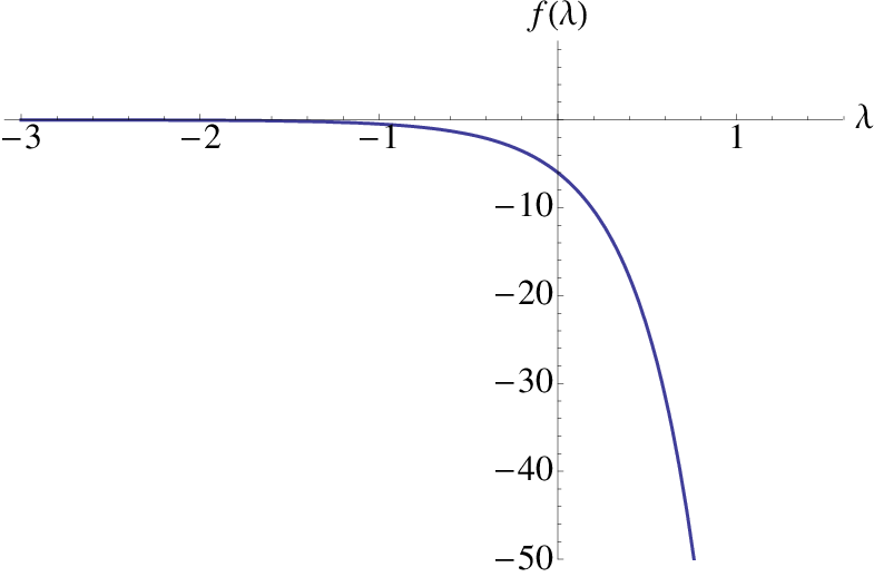
The negative sign signals that is asymptotically free. Inserting the fixed-point values from the Einstein-Hilbert sector in the Landau-DeWitt gauge with a spectrally adjusted cutoff (see App. A), we get . As long as the ghost anomalous dimension remains sufficiently small, our conclusion persists also for a larger truncation with a running ghost kinetic term.
Our result implies that (i) the non-Gaußian fixed point in the graviton sector is not influenced by the scalar curvature-ghost coupling, as the latter is zero at the fixed point, and (ii) this curvature-ghost coupling is RG relevant for the flow towards the IR. The latter property relates the initial value of this coupling to a physical parameter that has to be fixed by an RG condition (i.e., by an experiment). This does not necessarily imply that the scalar curvature-ghost coupling gives rise to an independent physical parameter. Since the background-field effective action has to satisfy (regulator-modified) Slavnov-Taylor and background-field identities [13, 15, 16, 17, 18, 44], this operator may be related to other purely gravitonic operators. An answer to this question requires to resolve the difference between background-metric and fluctuation-metric dependencies which is beyond the scope of this work.
Note that our arguments straightforwardly generalise to the coupling of any operator of the form , where is a scalar operator of some fields, e.g., matter fields. The interaction part of the corresponding flow will always have a contribution which supports an anti-screening flow. Of course, other contributions such as other interaction terms, the anomalous dimensions of the matter fields, and dimensional rescaling terms can eventually win out over the gravitational contributions.
IV Conclusions
We have contributed another building block to the asymptotic-safety scenario for Quantum Einstein Gravity by computing the RG flow of a scalar curvature-ghost coupling with the aid of the functional renormalisation group. In our present truncation involving an Einstein-Hilbert sector, a classical ghost kinetic term, and the curvature-ghost interaction, the coupling is found to be asymptotically free and RG relevant. Therefore, it belongs to the conjectured finite set of physical parameters which have to be fixed for an otherwise fully predictive theory of quantum gravity.
As this curvature-ghost coupling is marginal in a perturbative power-counting scheme, the relevance of this coupling at the non-Gaußian fixed point of the Einstein-Hilbert system is another example of the tendency of the fixed-point theory to increase the critical exponents of operators towards the RG relevant regime.
From a technical viewpoint, we have shown that a direct integration of gravity fluctuations in the functional RG equation is possible without relying on heat-kernel traces and propertime representations. As little is known about heat-kernel expansions with respect to ghost operators, a running ghost sector has not been included in an asymptotic-safety study of gravity up to now. However, ghost operators or a more general gauge-fixing sector may carry important pieces of information about the flow of a theory in certain gauges, as it is the case, e.g., in Landau-gauge Yang-Mills theory in the strong-coupling domain. We believe that a more detailed investigation of the ghost sector is important for a better understanding of the non-Gaußian fixed-point regime of Quantum Einstein Gravity.
For instance, an evaluation of the ghost wave function renormalisation is still an open question, but at the same time of primary importance as it will both feed back into the Einstein-Hilbert sector as well as take influence on the curvature-ghost coupling studied here.
Acknowledgements.
The authors would like to thank D.F. Litim, J.M. Pawlowski, and F. Saueressig for helpful discussions. This work was supported by the DFG under contract No. Gi 328/5-1 (Heisenberg program), FOR 723, and GK 1523.Appendix A Einstein-Hilbert sector
In this appendix, we summarise the results obtained from applying our technique to the flow of the Einstein-Hilbert sector. As the combination of the Landau-DeWitt gauge together with the spectrally adjusted regulator has not been used before, our results represent an independent verification of the fixed-point scenario.
The spectrally adjusted flow equation has the following form in the Einstein-Hilbert sector
| (36) |
where
| (37) |
Here, is the set of all modes of the York decomposition of the graviton as well as the ghost. We have also introduced a normalising factor which is chosen such that numerical factors in front of the eigenvalue of in the inverse propagator cancel in . This guarantees that all Lanplacean momentum modes are regularised by the same effective IR cutoff scale. In order to regularise the conformal instability, may also acquire a negative sign.
Inserting the propagators and using the Euler-MacLaurin formula for evaluating the spectral traces, we project onto the two running couplings in the Einstein-Hilbert sector. E.g., in four dimensions, is accompanied by a factor of the curvature radius squared, whereas the combination comes with a factor of . This allows for a straightforward projection and yields the following functions of the dimensionless couplings:
| (38) | |||||
| (39) | |||||
Note that branch cuts in the logarithm and the polylogarithm contribute imaginary parts which cancel for . Thereby, the flow equations are completely real for all values of . At the fixed point, and , implying (for )
| (40) | |||||
| (41) |
A numerical solution yields the following fixed-point values
| (42) |

The universal value is very close to the numerical values from other gauges and regulators [34]. The eigenvalues of the stability matrix correspond to the critical exponents at the fixed point (apart from a minus sign). In the present truncation, they appear as a complex conjugate pair,
| (43) |
inducing a spiral shape of the flow lines in the vicinity of the NGFP, see Fig. 3.
References
- [1] G. ’t Hooft and M. J. G. Veltman, Annales Poincare Phys. Theor. A 20, 69 (1974).
- [2] M. H. Goroff and A. Sagnotti, Phys. Lett. B 160, 81 (1985).
- [3] A. E. M. van de Ven, Nucl. Phys. B 378, 309 (1992).
- [4] S. M. Christensen and M. J. Duff, Nucl. Phys. B 170, 480 (1980).
- [5] J. Ambjorn, J. Jurkiewicz and R. Loll, Phys. Rev. Lett. 95, 171301 (2005) [arXiv:hep-th/0505113].
- [6] J. Ambjorn, J. Jurkiewicz and R. Loll, Phys. Lett. B 607, 205 (2005) [arXiv:hep-th/0411152].
- [7] J. Ambjorn, J. Jurkiewicz and R. Loll, Phys. Rev. Lett. 93, 131301 (2004) [arXiv:hep-th/0404156].
- [8] S. Weinberg, In *Hawking, S.W., Israel, W.: General Relativity*, 790-831
- [9] S. Weinberg, arXiv:hep-th/9702027.
- [10] S. Weinberg, arXiv:0903.0568 [hep-th].
- [11] C. Wetterich, Phys. Lett. B 301, 90 (1993).
- [12] C. Wetterich, Nucl. Phys. B 352, 529 (1991).
- [13] M. Reuter, Phys. Rev. D 57, 971 (1998) [arXiv:hep-th/9605030].
- [14] M. Reuter and C. Wetterich, Nucl. Phys. B 417, 181 (1994).
- [15] M. Reuter and C. Wetterich, arXiv:hep-th/9411227.
- [16] M. Reuter and C. Wetterich, Phys. Rev. D 56, 7893 (1997) [arXiv:hep-th/9708051].
- [17] J. M. Pawlowski, Annals Phys. 322, 2831 (2007) [arXiv:hep-th/0512261].
- [18] H. Gies, arXiv:hep-ph/0611146.
- [19] W. Souma, Prog. Theor. Phys. 102, 181 (1999) [arXiv:hep-th/9907027].
- [20] O. Lauscher and M. Reuter, Phys. Rev. D 65, 025013 (2002) [arXiv:hep-th/0108040].
- [21] M. Reuter and F. Saueressig, Phys. Rev. D 65, 065016 (2002) [arXiv:hep-th/0110054].
- [22] D. F. Litim, Phys. Rev. Lett. 92, 201301 (2004) [arXiv:hep-th/0312114].
- [23] L. N. Granda and S. D. Odintsov, Grav. Cosmol. 4, 85 (1998) [arXiv:gr-qc/9801026].
- [24] O. Lauscher and M. Reuter, Class. Quant. Grav. 19, 483 (2002) [arXiv:hep-th/0110021].
- [25] O. Lauscher and M. Reuter, Phys. Rev. D 66, 025026 (2002) [arXiv:hep-th/0205062].
- [26] P. F. Machado and F. Saueressig, Phys. Rev. D 77, 124045 (2008) [arXiv:0712.0445 [hep-th]].
- [27] A. Codello, R. Percacci and C. Rahmede, Annals Phys. 324, 414 (2009) [arXiv:0805.2909 [hep-th]].
- [28] P. Forgacs and M. Niedermaier, arXiv:hep-th/0207028.
- [29] M. Niedermaier, JHEP 0212, 066 (2002) [arXiv:hep-th/0207143].
- [30] M. Niedermaier, Nucl. Phys. B 673, 131 (2003) [arXiv:hep-th/0304117].
- [31] A. Codello, R. Percacci and C. Rahmede, Int. J. Mod. Phys. A 23, 143 (2008) [arXiv:0705.1769 [hep-th]].
- [32] D. Benedetti, P. F. Machado and F. Saueressig, arXiv:0901.2984 [hep-th].
- [33] M. Niedermaier and M. Reuter, Living Rev. Rel. 9, 5 (2006).
- [34] D. F. Litim, arXiv:0810.3675 [hep-th].
- [35] R. Percacci, arXiv:0709.3851 [hep-th].
- [36] E. Manrique and M. Reuter, arXiv:0905.4220 [hep-th].
- [37] T. Kugo and I. Ojima, Prog. Theor. Phys. Suppl. 66 (1979) 1.
- [38] V. N. Gribov, Nucl. Phys. B 139, 1 (1978).
- [39] D. Zwanziger, Phys. Rev. D 69 (2004) 016002.
- [40] R. Alkofer and L. von Smekal, Phys. Rept. 353, 281 (2001); [arXiv:hep-ph/0007355].
- [41] C. S. Fischer, J. Phys. G 32, R253 (2006) [arXiv:hep-ph/0605173].
- [42] A. K. Das and M. Kaku, Nuovo Cim. 50B, 303 (1979).
- [43] L. F. Abbott, Nucl. Phys. B 185, 189 (1981).
- [44] F. Freire, D. F. Litim and J. M. Pawlowski, Phys. Lett. B 495, 256 (2000) [arXiv:hep-th/0009110].
- [45] U. Ellwanger, M. Hirsch and A. Weber, Z. Phys. C 69, 687 (1996).
- [46] D. F. Litim and J. M. Pawlowski, Phys. Lett. B 435, 181 (1998).
- [47] J. W. York, J. Math. Phys. 14, 456 (1973).
- [48] M. A. Rubin and C. R. Ordonez, J. Math. Phys. 26, 65 (1985).
- [49] M. A. Rubin and C. R. Ordonez,
- [50] H. Gies, Phys. Rev. D 66, 025006 (2002) [arXiv:hep-th/0202207].
- [51] P. Fischer and D. F. Litim, AIP Conf. Proc. 861, 336 (2006) [arXiv:hep-th/0606135].
- [52] P. Fischer and D. F. Litim, Phys. Lett. B 638, 497 (2006) [arXiv:hep-th/0602203].