A new intrinsic numerical method for PDE on surfaces Thanks:  Partially supported by NSC, Taiwan

We consider a parameterization $x:U\rightarrow\Sigma$ at a point $p$, where $U$ is an open subset of the 2D Euclidean space $\mathbb{R}^{2}$. We can choose, at each point $q$ of $x(U)$, a unit normal vector $N(q)$. The map $N:x(U)\rightarrow S^{2}$ is the local Gauss map from an open subset of the regular surface $\Sigma$ to the unit sphere in the 3D Euclidean space $\mathbb{R}^{3}$. The Gauss map $N$ is differentiable. Denote the tangent space of $\Sigma$ at the point $p$ by $T\Sigma_{p}=\{v\in\mathbb{R}^{3}:v\bot N(p)\}$. The tangent space $T\Sigma_{p}$ is a linear space spanned by $\{x_{u},x_{v}\}$ where $u,v$ are coordinates for $U$.

The gradient $\nabla g$ of a smooth function $g$ on $\Sigma$ can be computed from

where $E$, $F$, and $G$ are the coefficients of the first fundamental form and

See do Carmo[7] for the details. Note that the gradient $\nabla g$ assigns to each point $q$ in $\Sigma$ a tangent vector $\nabla g(q)$ such that we have for all $v\in T\Sigma_{q}$,

where the smooth curve $\gamma(t)$ is in $\Sigma$ with $\gamma(0)$ and $\gamma^{\prime}(0)=v$.

The LB operator $\triangle$ acting on the function $g$ is defined by the integral duality

for all smooth function $\phi$ on $\Sigma$. A direct computation yields the following local representation for the LB operator on a smooth function $g$:

To move from regular surfaces to triangular meshes, one need to avoid the problem of local parametrization $x$ around a vertex $p$. In other word, one does not have the fist fundamental form $E$, $F$, $G$ and their derivatives for the computation of the gradient and the Laplacian operator of a function on a triangular mesh. To handle this problem, we give a novel method in Chen, Chi and Wu[5] to compute these differential quantities. The primary ideas were developed in Chen, Chi and Wu[4] where we try to estimate the discrete partial derivatives for 2D scattered data points.

In this section we shall describe a unified, simple and effective method to define the discrete gradient and the discrete Laplacian operator on functions on a triangular mesh. The primary ideas were developed in Chen, Chi and Wu[3, 4] where we try to estimate the discrete partial derivatives of functions on 2D scattered data points. Indeed, the method that we shall use to develop our algorithm is divided into two main steps: first we lift the 1-neighborhood points to the tangent space and obtain a local tangential polygon. Second, we use some geometric idea to lift functions and vectors to the tangent space and then we can compute their derivatives in the 2D tangent space. This means that the lifting process allows us to reduce the 2D curved surface problem to the 2D Euclidean problem and hence the methods in [4] and[8] can be applied.

Consider a triangular mesh $S=(V,F)$, where $V=\{v_{i}|1\leq i\leq n_{V}\}$ is the list vertices and $F=\{f_{k}|1\leq k\leq n_{F}\}$ is the list of triangles. Next, we introduce the notion of the local tangential polygon $P(v)$ at the vertex $v$ of $S$ as follows:

1. 1.

   The normal vector $N(v)$ at the vertex $v$ in $S$ is given by

   $$N(v)=\frac{\sum_{f\in T(v)}\omega_{f}N_{f}}{\left\|\sum_{f\in T(v)}\omega_{f}N_{f}\right\|}$$

   (6)

   where $N_{f}$ is the unit normal to a triangle face $f$ and the centroid weight is given in [2] by

   $$\omega_{f}=\frac{\frac{1}{\|G_{f}-v\|^{2}}}{\sum_{\tilde{f}\in T(v)}\frac{1}{\|G_{\tilde{f}}-v\|^{2}}}.$$

   (7)

   Here, $G_{f}$ is the centroid of the triangle face $f$ determined by

   $$G_{f}=\frac{v_{i}+v_{j}+v}{3}.$$

   (8)

2. 2.

   The tangent plane $TS(v)$ of $S$ at $v$ is now determined by

   $$TS(v)=\{w\in\mathbb{R}^{3}|w\bot N(v)\}.$$

   (9)

3. 3.

   The local tangential polygon $P(v)$ of $v$ in $TS(v)$ is formed by the vertices $\tilde{v}_{i}$ which is the lifting vertex of $v_{i}$ adjacent to $v$ in $S$.

   $$\tilde{v}_{i}=(v_{i}-v)-<v_{i}-v,N(v)>N(v).$$

   (10)

   as in figure 1.

Let $h$ be a function on $V$. We will lift locally the function $h$ to a function, denoted by $\tilde{h}_{v}$, on the vertices $\tilde{v}_{i}$ in $P(v)$ by simply setting

And $\tilde{h}_{v}(\vec{0})=h(v)$ where $\vec{0}$ is the origin of $TS(v)$. One can then extend the function $\tilde{h}_{v}$ to a piecewise linear function, still denoted by $\tilde{h}_{v}$, on $P(v)$ as follows.

Consider a face $f$ with vertices $v$, $v_{i}$ and $v_{j}$ in $F$. We obtain a lifting face $\tilde{f}$ with vertices $\vec{0}$, $\tilde{v}_{i}$ and $\tilde{v_{j}}$ in $P(v)$. Every point $p$ in $\tilde{f}$ can be written as a linear combination of $\tilde{v}_{i}$ and $\tilde{v_{j}}$ . That is, $p=a\tilde{v}_{i}+b\tilde{v}_{j}$ where $a,b\geq 0$ and $a+b\leq 1$. Then we define

Hence, the extended function $\tilde{h}_{v}$ is affine on each triangle $\tilde{f}$ of $P(v)$ and is differentiable on $\tilde{f}$. The gradient $\nabla(\tilde{h}_{v})_{\tilde{f}}$ of $\tilde{h}_{v}$ at the origin $\vec{0}$ can be obtained by

where the coefficients $\alpha$ and $\beta$ satisfy the relations:

As easy computation gives

To obtain the gradient $\nabla h(v)$ of $h$ on $S$ at the vertex $v$, we use again the weighted combination method. Namely, we set

with

where $G_{\tilde{f}}$ is the centroid of the lifting triangle face $\tilde{f}$ and is determined by

Next we explain how to obtain a good discrete Laplacian $\triangle h(v)$ of a function $h$ on the triangular mesh $S$. From the discussions above, we obtain the gradient $\nabla h(v)$ of $h$ on $S$ at each vertex $v$. We can use the method of parallel transport to lift the vector $\nabla h(v_{i})$ at $v_{i}$ to a vector $\nabla\tilde{h}(\tilde{v}_{i})$ in the tangential space $TS(v)$. The idea is to define a orthonormal linear map from $TS(v_{i})$ to $TS(v)$. To do so, we choose an orthonormal basis for $TS(v)$ by

The corresponding orthonormal basis for $TS(v_{i})$ is then given by

Then, the linear map $L$ of the parallel transport is given by

for $w=a\tilde{e}_{1}+b\tilde{e}_{2}$ in $TS(v_{i})$. See figure 2.

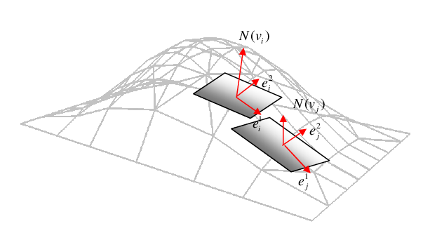
In this way, we can set the tangential gradient $\nabla\tilde{h}$ at $\tilde{v}_{i}$ by

Hence we obtain a tangential gradient $\nabla\tilde{h}$ of $h$ at each vertex $\tilde{v}_{i}$ in the tangential polygon $P(v)$ and we also set

See figure 3.

Fix an orthonormal basis $\{e_{1},e_{2}\}$ for $TS(v)$. The tangential gradient $\nabla\tilde{h}$ can be written as

The coefficients $a(\tilde{v}_{i})$ and $b(\tilde{v}_{i})$ can now be viewed as functions on the vertices $\tilde{v}_{i}$ of the tangential polygon $P(v)$. As before, we can then obtain their gradients $(\nabla a)(\vec{0})$ and $(\nabla b)(\vec{0})$ at origin. Namely,

with the centroid weights $\omega_{\tilde{f}}$ as in (17).

Put them in the matrix form to give

Therefore we have the Laplacian $\triangle h(v)$ of $h$ at the vertex $v$ of $S$ :

Theoretically the definition of the Laplacian $\triangle h(v)$ is independent of the choice of the orthonormal basis $\{e_{1},e_{2}\}$.

References

- [1] Bertalmio, M. Sapiro, G. Cheng L.T. and Osher, S. A framework for solving surface partial differential equations for computer graphics applications.(2000) CAM Report00-43, UCLA, Mathematics Department.
- [2] Chen, S.-G., Wu, J.-Y.. Estimating normal vectors and curvatures by centroid weights.(2004) Computer Aided Geometric Design vol 21, pp. 447-458.
- [3] Chen, S.-G., Chi, M.-H., Wu, J.-Y.. Curvature estimation and curvature flow for digital curves.(2006) WSEAS transcations on computers, vol 5, p804-809.
- [4] Chen, S.-G., Chi, M.-H., Wu, J.-Y.. Boundary and interior derivatives estimation for 2D scattered data points.(2006) WSEAS transcations on computers, vol 5, p824-829.
- [5] Chen, S.-G., Chi, M.-H., Wu, J.-Y.. On a new differential method for triangular meshes.(2009) preprint.
- [6] Dorsey, J. and Hanrahan, P.. Digital materials and virtual weathering.(2000) Scientific American 282:2, pp46-53
- [7] do Carmo, M.. Differential Geometry of curves and surfaces.(1976) Prentice Hall, Englewood Cliffs, NJ.
- [8] Hiroshi Akima, On estimating partial derivatives for bivariate interpolation of scattered data, Rocky Mountain Journal 14 (1984), pp. 41-52, MR0736165.
- [9] Taubin, G.. A signal processing approach to fair surface design.(1995) In SIGGRAPH’95 Proceedings, pp. 351-358.
- [10] Taubin, G.. Estimating the tensor of curvatures of a surface from a polyhedral approximation.(1995) In: proceedings of the Fifth International Conference on Computer Vision, pp. 902-907.
- [11] Turing, A.. The chemical basis of morphogenesis.(1952) Philosophical Transactions of the Royal Society B 237, pp.37-72.
- [12] Turk, G.. Generating textures on arbitrary surfaces using reaction-diffusion.(1991) Computer Graphics (SIGGRAPH) 25:4,pp. 289-298.
- [13] Witkin, A. and Kass, M.. Reaction-diffusion textures.(1991) Computer Graphics (SIGGRAPH) 25:4,pp. 299-308