Throughput Improvement and Its Tradeoff with The Queuing Delay in the Diamond Relay Networks
Abstract
Diamond relay channel model, as a basic transmission model, has recently been attracting considerable attention in wireless Ad Hoc networks. Node cooperation and opportunistic scheduling scheme are two important techniques to improve the performance in wireless scenarios. In the paper we consider such a problem how to efficiently combine opportunistic scheduling and cooperative modes in the Rayleigh fading scenarios. To do so, we first compare the throughput of SRP (Spatial Reused Pattern) and AFP (Amplify Forwarding Pattern) in the half-duplex case with the assumption that channel side information is known to all and then come up with a new scheduling scheme. It will that that only switching between SRP and AFP simply does little help to obtain an expected improvement because SRP is always superior to AFP on average due to its efficient spatial reuse. To improve the throughput further, we put forward a new processing strategy in which buffers are employed at both relays in SRP mode. By efficiently utilizing the links with relatively higher gains, the throughput can be greatly improved at a cost of queuing delay. Furthermore, we shall quantitatively evaluate the queuing delay and the tradeoff between the throughput and the additional queuing delay. Finally, to realize our developed strategy and make sure it always run at stable status, we present two criteria and an algorithm on the selection and adjustment of the switching thresholds .
Index Terms:
diamond relay networks, cooperative pattern, block Rayleigh fading, finite state channel, G/G/1 queueing system, tradeoff.I Introduction
In recent years, motivated by higher quality-demanded applications in the wireless Ad Hoc networks, cooperation among nodes is considered to be more useful over various relay network models. Early in 1970s, a classical three-node relay channel comprised of one source, one destination and only one relay was first introduced by van de Meulen in [3]. Then, in reference [4] and [5], the cut-set bound and the achievable rates with power allocation were studied for the half-duplex case in this three-node network. Especially, Reference [5] presented some lower and upper bounds on outage capacity of three-node network. The analysis of diversity-multiplexing tradeoff for the three-node network in the half-duplex case was given in [6]. Besides, systems using multiple relays were also studied. In [7], both the achievable rates and the upper bound of capacity were studied for the diamond relay network in the half-duplex case. The two-relay model (i.e. the Diamond Relay Networks) operating in the full-duplex case were studied in [8]. In [9], they analyzed a model in which cooperative communication proceeds in a parallel relay network where the exogenous arrival of packets and the FIFO (First In First Out) queueing system are introduced. Multiple relays using orthogonal channels were analyzed in [10]. Besides, relay networks with and without delay were discussed in [12] and [13], respectively. Reference [14]-[19] presented analysis of capacity and delay tradeoff in the networks comprised of many random prelocated nodes. These works showed that a cooperative gains can be obtained in distributed wireless networks if nodes can help each other to relay information. This motivated us to study the wireless relay networks further, especially for some classical topologies and cooperative modes.
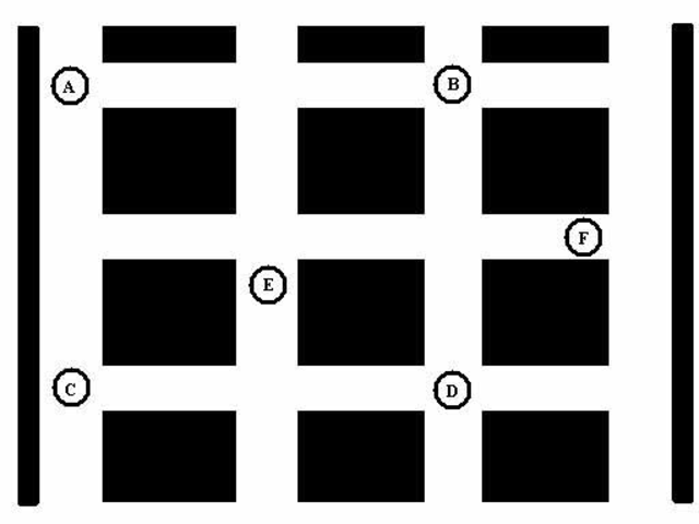
Referring to the wireless relay networks, the three-node network has been a very hot topic in the research area of the cooperative network since 1970s due to its classical and representative topology. In the late ninety’s, B.Schein and R.Gallager proposed another kind of relay network, the Gaussian parallel relay network [8], in which the diamond relay network was first introduced implicitly. The reasons that diamond relay networks were considered include two facets: Firstly, this kind of topology is relatively easy traceable in theory and has more freedom than three-node network model. Secondly, this model can be used in some wireless scenarios, where a sender is convenient to select a few neighbors. Fig. 1 shows one application scenario where the black and square parts represent the obstacles blocking radio signals seriously, e.g., skyscrapers in business district. In such a scenarios, if node A wants to transmit to node D at a higher rate, the diamond relay network comprised of node A,B,C and D can do a great help.
Based on different topologies of the wireless relay networks [3]-[8],[10], several cooperative modes were introduced consequently, such as SRP (Spatial Reused Pattern) and AFP (Amplify Forwarding Pattern) in [7]. In the wireless time-varying and fading scenarios, different cooperative modes may have big difference in term of reliable throughput where opportunistic scheduling may play a key role in improving the throughput. Motivated by this, we firstly review the two different cooperative modes, namely SRP and AFP, and present their corresponding capacities in the diamond relay network, shown in Fig. 2, in the half-duplex case. In the discussion, relay nodes adopt two relay schemes, namely, the amplify-and-forward (AF - relay node simply amplifies the signals received from source and forwards to destination) and decode-and-forward (DF - relay node decodes the information received from source, re-encodes and forwards to destination). In the sequel, AF relay scheme is referred to AFP (Amplify Forwarding Pattern) mode while DF relay scheme is referred to SRP(Spatial Reused Pattern) mode. Furthermore, we compare the throughput of the two cooperative modes and find that there exists a big difference between the performances of the SRP and AFP mode. In some cases, SRP has a larger throughput than AFP. Otherwise, it has smaller throughput than AFP. Thus, our first contribution is that we analyze the efficiency of opportunistic scheduling and put forward a hybrid relay scheme with switching between SRP and AFP so that it can be adapted to the channel variation.
Although the opportunistic scheduling is usually considered to be effective, it will be shown that combining SRP and AFP in a simple way can not obtain an expected improvement. This is because SRP is always superior to AFP on average due to the efficient spatial reuse. In previous works [3]-[8], using Max-Flow Min-Cut theorem, it can be seen that the whole performance is always reduced greatly by some bottleneck links usually caused by the fading and time-vary characteristics of the wireless channels. Therefore, using buffers at nodes maybe help to efficiently employ some channels in rather good conditions. In this way, it will improve the whole performance of the throughput in the wireless networks at the cost of some additional queuing delay. Motivated by this, we shall put forward a new processing strategy in which buffers are employed at both relays in SRP mode. Its basic idea is that in diamond relay channels, sometimes there is only one or two links in very good conditions while the others in bad ones. In this case, buffers can help relays efficiently utilizing the links in good conditions so that the throughput is greatly improved at some cost of queuing delay. One important contribution of this work is that we quantitatively evaluate the queuing delay and discuss its tradeoff with the throughput where two criteria are considered to characterize the thresholds for separating pretty good or rather bad condition of channels and make sure the network run in stable status. In addition, an adjust algorithm is also given.
For simplicity, finite state channel model is used in which the received SNR is partitioned into levels. The status of the four links are assumed to be independent and each link operates in a memoryless mode. G/G/1 queueing system is used to model the relay node with buffers and the associated two links connecting to it. Besides, a continuous traffic model is considered in which the source always has information to send. Then one can use Marshall’s theory to solve it. Note that here we consider the source always has information to send, which will help us to get more insights on the maximum achievable throughput of this diamond network. Thus, other traffic models, such as Bernoulli or Poisson traffic model, will not be discussed here. Another point should be mentioned is that due to the IC design improvement, buffers with enough capacity are becoming much cheap and with low cost, so the delay is a more rigorous factor influencing the performance of the networks. Therefore we emphasize the average queuing time without limitation of the buffer sizes, referred to delay in this paper.
The rest of this paper is organized as follows: In Section II, we introduce the system model. In Section III, we firstly compare the performance of SRP and AFP scheme,then we give an opportunistic scheduling scheme, namely an hybrid scheme of combining SRP and AFP modes. In Section IV, we shall propose a new processing strategy in which buffers are employed at the relay nodes in SRP mode. We present two criteria to characterize the thresholds for realizing tradeoff between the throughput and queuing delay and make sure the network run in stable status. Some simulation results are given in Section V. Finally, We present the conclusion in section VI.
II System Model
II-A Diamond Relay Channel and Two Time Sharing Patterns: SRP and AFP
The discussion of diamond relay channel was first considered in
Schein and Gallager’s work in a full-duplex case [8]. Recently,
Feng, etc, studied this kind of networks in the half-duplex case in
[7], shown in Fig. 2. It is comprised of four nodes including a
source , two relays and and a destination . It
is assumed that all four nodes operate in half-duplex mode, and that
the destination can not communicate with the source directly and the
two relay nodes will not interfere with each other [7]. Now we first
review the two cooperative modes, namely SRP and AFP, as follow.
SRP: A time block, , is divided into two stages.
- 1.
Stage 1: In the first slots, source node and relay node transmit signals while relay node and destination node are in receiving status. is time sharing parameter.
- 2.
Stage 2: In the remaining slots, source node and relay node transmit signals while relay node and destination node are in receiving status.
AFP: A time block is also divided into two stages.
- 1.
Stage 1: In the first slots, source node transmit signals while both relays and are in receiving status. In this case, the destination can not hear the signal.
- 2.
Stage 2: In the next slots, both relays and forward the received signals in the first time slots while the destination is in receiving status and source node keeps silent.
Let and denote the signal sent by node and that received by node , respectively. Then the equivalent baseband signals of the two cooperative modes are given by, respectively,
- 1.
In SRP:
In the first slots:
In the remained slots: - 2.
In AFP:
In the first slots:
In the remained slots:
where are independent and identically distributed (i.i.d) circular Gaussian random variables. is the gain factor of the link from node to node . In the discussion, all the nodes are power limited. Their maximum transmitted are assumed to be the same, denoted as . Here the channel side information is used by receivers feedback few bits reflecting the link conditions. The bit number is relatively little compared to the data packets. For instance, one relay can first estimate the status of the two links associated to it and then feedback to the source and the destination. The source will inform the status of this link to another relay in next time slot by adding a overhead in its traffic massage. This process renews only once at the beginning of each time block according to the block channel fading. In this way, all the nodes could obtain the channel side information and cooperate in this time block, , which consists of many time slots.
II-B Finite State Fading Channel
To effectively analyze the fading and time-variant characteristics of channels, a finite state fading model is built by partitioning the instantaneous received SNR into N levels. Some partition methods , such as the equal-probability partition method [20], the optimum Minimum Mean-Square Error (MMSE) Lloyd-Max quantification method etc. have been employed previously. For simplicity, we shall adopt an equal-probability partition and use its mean value of SNR to represent the exact SNRs in each interval [20] here. Note that it will be consistent with the real case as the partition level is large enough.
Let denote the probability of link state and denote the partition boundary of each state, which is determined by
| (1) | |||
| (2) |
where is the of the received SNR over a Rayleigh channel and is the reciprocal of the average received . The mean value of SNRs in each interval, ,, is given by
| (3) |
The maximum average rate of the link at the state level i is given by .
In the paper, we assume that the maximum rate can be approximately achieved by some effective pseudo-random channel coding schemes and that the destination node can receive the signals from the two relays coherently in the AFP model. Thus, we use the corresponding capacity to approximately trace the maximum achievable transmitting rate. For simplicity, let denote the maximum achievable rate in the sequel.
II-C Block Rayleigh Fading Model
It is assumed that the channels endure block fading, which means that the received SNR in one time block is a constant, but it may vary from block to block obeying the exponential distribution, which is corresponding to Rayleigh fading. Furthermore, the states of the four links are assumed to be independent and for each link its SNR varies according to a memoryless mode.
II-D Marshall’s Queueing Theory
For G/G/1 model, Marshall’s theorem on the estimation of the average queuing time is reviewed here [11].
Theorem : For all G/G/1 queues with , we have
| (4) |
where and denote the arrival interval and the service time, respectively. and denote the corresponding variances of them, respectively. is the average traffic arrival rate and is the traffic intensity of the system. and are the first and second order moments of the idle period of the system.
If the inequality holds, the upper bound of the waiting time is given by
| (5) |
Note that the inequality becomes an equality when approaches .
III Opportunistic Scheduling Scheme Combining SRP and AFP
To compare the performance of cooperative modes, SRP and AFP, we
first analyze the capacity of the SRP and AFP. For convenience,
several symbols are defined first.
(1) is defined as and
(2) are defined as follows,
respectively. ,
.
III-A Capacity of SRP and AFP Modes
The SRP mode is a 2-hop strategy in which relay nodes decode their recdeived information first before re-transmitting to the destination. It is an efficient cooperative scheme for the diamond relay model due to the full spatial reuse. In the AFP mode, both relay nodes just amplify the signals received in the first half of T and re-transmit it in the next one. At each relay node, the signal is multiplied with a constant and the amplified signals from the two relay nodes are coherently added up at the destination if the timing synchronization and carrier recovery are perfect. In both modes, no buffer is used by the relay nodes. The maximum achievable transmission rate is based on the capacities between the links associated to the relay nodes.
Theorem :[7,Theorem4.1 and 5.2] (i) In SRP mode, denotes the capacity of the link from node to node . Transmitting rate of the link is denoted as and the one of the link is denoted as . The capacity of the SRP mode denoted as , which also represents the maximum achievable rate, is given by
| (6) | |||||
in which and .
In addition, the link-state space can be divided into four different subspace according to the following conditions (7) (8) (9) and (10). The explicit expression of capacity for the SRP mode in each case is given as follow.
| (10) | |||||
(ii) In AFP mode, parameter and denote the amplified factors at relay node and , respectively. Since the signals are received coherently, the maximum achievable rate is
| (11) | |||||
The first factor is due to the equal time-sharing and the first inequality becomes equality when holds.
Based on the theorem above, one can compare the maximum achievable rate of the two cooperative modes. However, Theorem 3.1 only consider the case where all the link capacity are fixed. If all the links are time varying, it is possible for us to select an effective processing mode adapted to the variation of the links so that we can get larger throughput by using buffers at relay nodes, which will shown later. Numerical results in Fig. 5 indicate that the upper bound of in Eqn.(11) is much smaller than on average. In addition, a general form of will be given in Appendix (B).
III-B Comparison Between SRP and AFP and An Opportunistic Scheduling Scheme
Using Eqn.(6) and Eqn.(11), we can divide the link-state space spanned by the four channel gain factors, , into eight different subspace. In each subspace, the capacity for both SRP and AFP modes are completely determined. Now, let us see a special case on AFP.
Theorem : In AFP mode, the link-state space is divided into two different subspace by the following conditions, where is satisfied. The corresponding explicit expression of in each case is given by
| (12) | |||||
| (13) | |||||
The proof is given in Appendix (A), while a general expression of is given in Appendix (B).
Based on and , the maximum average achievable rate can be explicitly presented in theory for all the different subspace so that the comparison between them becomes traceable.
The whole link state space spanned by is divided into eight different subspace and they are given by
According to the above analysis, an effective hybrid scheme combining the SRP and AFP modes is presented here.
An Opportunistic Scheduling Scheme : In the diamond relay network model, if the channel side information is obtained by all the nodes at the beginning of each time block, it is possible to find the thresholds properly for subspace partition and select an effective cooperative mode with larger throughput.
Note that the switch between the two cooperative models will not be very frequent due to the block fading channel. It only occurs between two time blocks if necessary.
IV A New Processing Strategy With Buffers Employed by Relay Nodes
Numerical results in Fig. 5 indicated that SRP always performs much better than AFP on average due to its full spatial reuse. This means that only adopting a hybrid scheme simply can not bring an expected throughput improvement. Since the links associated to the relay is time-varying and block fading, some links in bad conditions will form a bottleneck, which greatly reduce the throughput. To overcome it, we shall put forward a new processing strategy in which buffers are used at both relays to efficiently use the links in good conditions, which is referred to opportunistic scheduling.
In fact, it is possible to find an effective opportunity scheduling under some cases, such as that only one or two links are in very good conditions while the others are all in bad conditions. Now we consider the following two cases shown in Fig. 3.
- 1.
At least one link from to the two relays are in pretty good conditions while the two links from the relays to destination are in rather bad conditions.
- 2.
At least one link from the two relays to destination are in pretty good conditions while the two links from source to the relays are in rather bad ones.
In Fig. 3, symbol denotes the link in pretty good conditions, denotes it in rather bad ones and denotes it in arbitary conditions (i.e. pretty good, rather bad or average). In this two cases, the links in rather bad conditions form the bottleneck of the networks, especially for those schemes without buffers. Therefore, the new opportunity scheduling scheme is expressed as follows.
New Strategy With Buffers Employed
(1) Under the above tow cases, we shall use these links with pretty good conditions to transmit signals while the links with rather bad conditions will keep silent and some received signals will be stored at its corresponding buffers.
(2) For other cases, we still adopt the same policy as that in hybrid scheme of combining SRP and AFP without buffers.
From the new opportunity scheduling scheme, one can find that a new raising problem is how to determine each link condition being good or bad? Furthermore, the evaluation of queuing delay caused by using buffers is a new problem to be considered. In the sequel, we shall deal with them.
IV-A Two Criteria for Selecting Threshold of Link Condition
Since the signals transmitted from source to both relays in AFP mode is the same and the destination needs to receive it coherently, no buffers in AFP mode may loss some opportunities to adapt the link time-varying conditions. For SRP mode, source will transmit different signals to the two relays, the sequence number of the received symbols at the destination may be different with its original ones due to these link time varying capacities, which is similar to the phenomenon in Internet. Furthermore, is mainly determined by the very bad links according to Theorem 3.2 when the conditions of the four links have much difference. Therefore, buffers employed in SRP mode for the two cases listed above can mitigate the impact of bottleneck links. In other cases, e.g., the conditions of the links are almost the same, no matter whether it is good or bad, the impact of bottleneck links is relatively small for SRP mode.
To separate the pretty good and rather bad link states, we first propose two thresholds of the link state levels, denoted as and , respectively, based on the finite state fading channel model. That is to say, the link is considered to be in pretty good condition if its state level is above or equal to and considered to be in rather bad condition if its state level is below or equal to .
| (14) |
Based on this criterion, we shall prove that only under the two cases discussed above, the throughput improvement can be obtained. The detail of proof is given in Appendix (C). Here we shall give an explanation for Criterion 1 in principle.
Consider two consecutive time blocks and , , and is prior to . For the hybrid scheme without buffers, the total amount of information transmitted in this two consecutive time blocks, denoted as , is given by
| (15) |
and for the new developed strategy, the total amount of information transmitted in this two consecutive time blocks, denoted as , is given by
| (16) |
Note that “” is to guarantee that the buffer is not empty while “” in Eqn. (16) means utilizing the better route. In fact, in a causal system, one can not obtain during the block , thus Eqn.(16) only presents an ideal case. In practice, we shall use the better front-side link associated to the two relays when case (1) happens. This is because the probabilities of different link states are equal and the link states change independently from one block to next, which means the two back-side links associated to the relays have the same probability being in pretty good conditions when case (2) happens. From statistic view of point, choosing the better front-side link and sending massage as much as possible will obtain a larger gain. In addition, if the buffer becomes empty as case (2) happens, the relay will not transmit any massage. This is the case just as that in a general G/G/1 system. Even though, the performance will degrade little because the throughput of those non-buffer strategies also become rather small when case (2) happens. Thus, we can still use Eqn.(16) in the following analysis approximately.
Let us observe the case that in only the link from to is pretty good and in only link from to is pretty good while all the other three links are rather bad, which means and hold. In this case, the throughput of the hybrid scheme without buffers is very small due to the existence of bottleneck links. But for the new developed strategy, since one buffer is employed by , the total throughput in the two time blocks becomes much larger due to the efficient utilization of the link from to in and the good link from to in .
Associated with that SRP mode is better than AFP on average, it can be concluded that if the inequality holds, then the total amount of information transmitted in these two consecutive time blocks with the buffer’s help will be larger than that in the original hybrid mode in a certain degree. For other cases except cases and , buffers will not be used and their corresponding throughput parts keep the same. Therefore, one can see that the new developed strategy will improve the average throughput. The proof of is given in Appendix (C). Its main idea is that holds in these two cases according to Theorem 3.1. If the condition in Criterion 1 is satisfied, the inequality will hold and the improvement of throughput can be guaranteed.
TABLE I shows the levels of 16-state partition of the fading channel obtained by the corresponding maximum achievable rate with the normalization for different received SNR. According to Criterion 1, is selected from the left side of for each link state level and is selected from the right side of for the corresponding state level. In addition, the two sides are formed symmetrically because the performance of original schemes is relatively good for the case that link state levels fall into the interval between and since the impact of the bottleneck only dominates when the link states differ a lot.
IV-B Delay Analysis
In the previous example, the two time blocks, and , are assumed to be consecutive. In fact, they may not be adjacent to each other according to the link state model. That is, the information in the buffer has to wait for transmission. On the other hand, due to the links being in Rayleigh fading, the probability of links in pretty good conditions is relatively low, resulting in a larger delay for information transmission. In the new developed strategy, the mean value of the delay for information transmission is mainly determined by the thresholds and . Based on the topological symmetry of the diamond relay networks, we only analyze the performance of the subsystem, shown in Fig. 4. In Table II, some notations are firstly defined.
with the link state model, and are given by
Note that the item is the probability that the condition of the link between and is better than that between and when they are both pretty good. In the new developed strategy, only if the link state falls into one of the two cases mentioned previously, the buffer works. In other cases, the buffer will not work and the networks run with the same procedure as the non-buffer scheme. That is, no new massage is put into the buffer though it is delivered to the corresponding relay node. The massage queuing in the buffer previously will wait for the moment at which cases (1) or (2) happen again. The details of the queuing model can be described as follows.
- 1.
Arrival process: Since the source always has information to deliver, the link state to the relay determines the input process of the buffer, refer to the arrival process of buffer, including the arrival interval and rate. When link state is at level , the arrival interval between the successive traffic units is equal to . The symbol is a parameter determined by the traffic types of source (i.e. bit, byte or packet), which is not a key point and for simplicity, let represent a packet.
- 2.
Service process: The service process refers to the delivering process of the message stored in the buffer of the relays to destination. Once a packet stored in the buffer is transmitted successfully, it is served. Thus, the link state between the relay and destination determines the service process, including the service interval and rate.
The arrival interval of traffic units needs to be considered for the following three cases: when the buffer works, the condition of the link to the relay is pretty good. When the buffer works, the condition of the link to the relay is rather bad; and that buffer does not work. The value of arrival interval and its corresponding probability for each case is
and for the service time, similar results are given by
It is easy to see that the distributions of the arrival and service interval do not obey the uniform or Poisson distribution,etc. They are general. Therefore, one can solve it with the G/G/1 queuing model. The mean values and variances are given in Theorem 4.1.
In fact, the stability of queueing in buffer is very important. To solve this problem, the traffic intensity of buffer, denoted as , should be less than . In the new strategy, the stability of buffer can be guaranteed by selecting the thresholds, and , following criterion 2:
| (17) |
The proof is given in the Appendix (D). Furthermore, one can easily infer that for the case “” or “”, the buffer is also stable. Besides, due to that the thresholds, and or and are relatively close to each other and the source node has a continuous traffic to deliver, the arrival rate of the buffer is then close to but smaller than the service rate. That is, the traffic intensity of the buffer, the ratio of the arrival rate to the service rate, approach to . Consequently, the upper bound of the average delay in Marshall’s theory become more effective.
Theorem : For the new developed strategy with buffers at both relay nodes, we have
| (18) |
| (19) | |||||
| (20) | |||||
| (21) |
where , , and are given by, respectively,
The proof is given in the Appendix (E). , presented the upper bound of the average delay, , which is a function of the thresholds , , and . Consequently, it provides an theoretical way to consider the good tradeoff between the average delay and the network throughput.
IV-C Tradeoff Between the Throughput and the Delay
Follow the above discussions in Subsections IV. A and IV. B, the new developed strategy can really improve the throughput by efficiently utilizing the pretty good links at a cost of queuing delay. Using the two criteria, for the fixed and , if a relatively lower and higher are selected, the throughput improvement is less than that with selection of a relatively higher and lower . This is because that in the former case the value of is less than the one in the latter case (see Appendix (F)). On the other hand, according to , the former case has a shorter delay due to its higher service rate. A similar result can be observed for selecting and under the condition that and are fixed. Simulations in Section V will also confirm this phenomenon.
To achieve a good tradeoff between the throughput and the delay, we shall present an algorithm to select the thresholds, and , which is summarized as follows.
Enumerative Algorithm :Due to that the nodes are able to know the partition of link states in advance and obtain the average received SNR at the beginning of each time block . In other words, they already have the side information in Table I.
- 1.
Step 1: Enumerate the combinations of and according to both of the criteria.
- 2.
Step 2: Estimate the average delay for each case via and find out all the possible combinations of and whose average delay is shorter than the requirement by the service traffic. Let us denote the available set as .
- 3.
Step 3: For all the possible pair of and belonging to , to achieve larger throughput the nodes select as low as possible and as high as possible or select as low as possible and as high as possible.
V Numerical Results
In this section, simulation is used to demonstrate our theoretical results. In the simulation part, the stream traffic model is employed and the source node is assumed to have massage to deliver always. The average received SNR of these two relays and the destination varies from 0dB to 10dB. The simulation period consists of time blocks, denoted by , where each time block is equal to . For the new developed strategy, the total amount of information received successfully by the destination is . Then, the average throughput of the new developed strategy is evaluated by . Since there are several selections of and for each average received SNR, we estimate the average throughput for each case under the same average received SNR. For the original schemes, similar procedure are done.
Fig. 5 shows the maximum achievable rates of SRP, AFP, the hybrid scheme and the new developed strategy with buffers for each average received SNR. Both the theoretical and simulation results indicate that if all the links have the same average SNR, SRP mode is always better than AFP mode. Consequently, the hybrid scheme simply combining both of them is almost equivalent to that only adopting SRP mode. Compared with the original schemes, the new developed strategy with buffers really improve the average throughput, e.g. there is an approximate increment of unit/s at the average received SNR of 4dB. That is about improvement. In addition, the improvement rate will decrease as the received SNR increases further. It is because that when the average capacity of each link increases under a higher SNR, the degree of the bottleneck link influence becomes smaller.
Fig. 6 illustrates the average delay under different received SNR, evaluated in terms of the number of . It is shown that for a fixed average received SNR, the average delay increases as the traffic intensity becomes larger and for a fixed traffic intensity, the average delay decreases as the average received SNR increases. For instance, when traffic intensity is , the delay in the average received SNR of 2dB is , while the delay in the average received SNR of 10dB, it is only . Also it can be seen that the simulated curve becomes much closer to the theoretical one as approaches to 1, which demonstrated that the upper bound derived in theory is effective.
Fig. 7 shows the tradeoff between the improvement of network throughput and the average delay, which is consistent with our theoretical predication. Some simulation results are also listed in Table III where the average received SNR is equal to . It is shown that if the required average delay by the traffic is no more than 20 time blocks, one can only obtain a throughput increment of 0.0311bit/s when the thresholds are selected as , , and . That is about improvement compared to the original value in Table I. A larger improvement can be obtained if the requirement of average delay becomes loose. One can see that when nodes select a lower and a higher or select a lower and a higher , the throughput improvement become larger while the delay becomes larger simultaneously. In addition, if the average delay approaches to infinity in the case that , , and , since it does not match the stable conditions, Criterion 2.
VI Conclusions
In this paper, the diamond relay mode was studied. We compared the throughput performance of the two classical cooperative modes, SRP (Spatial Reused Pattern) and AFP (Amplify Forwarding Pattern) under wireless scenarios with assumption that the channel side information is known to all the nodes. We analyzed the possibility to improve the throughput by employing buffers at relays and proposed an new opportunity scheduling scheme. In order to improve the network throughput while guaranteing the stable running of the whole network, we established two criteria on the selection of SNR thresholds and one adjustment algorithm on the tradeoff between the throughput improvement and the queueing delay. Simulation results confirmed the effectiveness of our theoretical analysis and our new developed opportunity scheduling method.
Acknowledgment
It was supported by NSFC/RGC Joint Research Scheme No.60831160524 and the open research fund of National Mobile Communications Research Laboratory, Southeast University, China.
Appendix (A)
Proof of Theorem : The original expression can be transformed into the equivalent form:
That means achieves its maximum when reaches its maximum under the three constraints above. With the three constraints, one can find that
| (22) | |||||
Thus, the expression of in Eqn.(22) is obtained.
Appendix (B)
The original problem above is equivalent to the following one,
| (23) |
where
To derive the maximum value of , we first have
| (24) |
then we solve the following equations,
| (25) | |||
| (26) |
Rewriting Eqn. (23), it is easily found that
This indicates that is a monotone increasing function of if and a monotone decreasing function of if . Similar results can be derived for .
In addition, we find that the two equations and can not hold simultaneously. Otherwise, , which resulting in contradiction. In fact, if holds, then will be guaranteed.
According to the expression of , we only need to prove holds. Since
we have
Similar result can be obtained for that case if holds, then will be true.
In addition, according to Eqn.(25) and (26), if holds, then is true and if holds, then is true. Now we can summarize different cases:
(1) For the case that :
If , then and . Otherwise, we divide it into two subcases: a) If holds, we have and . b) If holds, we have and . where “” denotes the larger one between and with the constraint that both of them are less or equal to . If anyone of them is above , its value is defined as .
(2) For the case that :
If , then we have and . Otherwise, we also divide it into two subcases. a) If , then we have and . b) If , then we have and .
(3) For other cases: achieves the maximum value if and .
Appendix (C)
Without loss of generality, let us consider the proof of case (a) shown in Fig. 3. ( i.e. At least a link from source to the relays is pretty good and the two links from the relays to destination are rather bad.) It is easily to check that the condition (9) in Theorem 3.1 is satisfied for case (a). Thus, the maximum achievable transmitting rate can be given by
| (27) |
where , and holds in case (a).
In addition, is a monotone increasing function of both and . Thus, we have
| (28) |
Likewise, similar proofs can be given for another three cases in Fig. 3. Finally, based on Criterion 1, we conclude that holds only in the cases (1) and (2) presented in Section IV.
Appendix (D)
Firstly we deduce the average arrival rate and service rate for the system shown in Fig. 4, denoted as and , respectively. According to the new developed strategy, only cases (1) or (2) happens, the buffers start to work. Therefore, the average transmitting rate when the link states are in pretty good and rather bad conditions can be derived as follow
Associated with the probabilities that the buffers is in working status, and , we have
| (29) |
| (30) |
Next we consider the two conditions expressed in Criterion 2, respectively.
(i) If and , holds, then we have
The first inequality above holds because is true. Associated with and , one can see that . Thus, the corresponding traffic intensity is less than 1, indicating that the queueing is stable.
(ii) If and , holds, then we have
Similarly, the first inequality above holds because is true. Check all the possible combinations in Table I according to Criterion 1 and for each case, one can see that is true.
Likewise, we can also verify the case of the 8-level and 32-level partition and make sure the conclusion holds based on the two Criteria. The explanation in principle is that the impact of the variation of the terms “” and “” to the plus-minus of the inequality is much more greatly than that exerted by the gap between the ’s value in for each case with equal partition. Thus, holds, which guarantees the corresponding traffic intensity is less than 1 and the queue is also stable.
Appendix (E)
Proof of Theorem : Here just give the proof of the
mean and variance of arrival interval , respectively, denoted as
and . Similar proof for the service time can follow this one.
(1) When the buffer works and the link state is higher or equal to
state level , we have
| (31) |
(2) When the buffer works and the link state is lower or equal to the state level , we have
| (32) |
(3) When the buffer does not work in the consecutive time blocks, we have
| (33) |
With the results above, we get .
The proof for the variance of the arrival interval is similar. For example, When the buffer works and the link state is higher or equal to state level , we have
| (34) | |||||
When the buffer works and the link state is lower or equal to state level , the proof of is similar and we omit it here. When the buffer does not work in the consecutive time blocks, we have
| (35) | |||||
By using the known results, for , ,
and
| (36) | |||||
we have
| (37) |
Finally, we get .
Appendix (F)
Consider the average throughput improvement in the two time blocks and mentioned in our discussion. It can be denoted as . In addition, according to the expression of , we need to find out the transmitting rate (i.e.the explicit value of ) in all the possible cases and their corresponding probabilities.
For the fixed and , if we choose , then subjected to Criterion 2. The probability that the buffer works, , in the two time blocks and is
| (38) |
In addition, if holds, the average transmitting rate, denoted as , is
| (39) |
and if holds, the average transmitting rate, denoted as , is given by
| (40) |
Summarizing the results above, we have . That is,
| (41) |
Let represent the throughput improvement when and are selected. Then
| (42) | |||||
Next we keep as a invariable. For the case that , and we have
| (43) | |||||
In order to prove that , we use the following way.
Based on , in the expression of , we replace the former items with and the latter items with , then we obtain the infimum of as follows
| (44) | |||||
In the expression of , we replace the former items with and the latter items with , then we get supremum of as follows
| (45) | |||||
where .
Now by scaling and further according to , we have
| (46) | |||||
| (47) | |||||
From the deductions above, the proof of is equivalent to the proof of .
Using the result in Appendix (D), we have . From Table 1, we find that always holds for all the cases of average SNR if . Furthermore,
| (48) |
This indicates that to prove , we only need to analyze the expression . In fact, if the following inequality holds,
| (49) |
the inequality will be true.
According to Table 1, we obtain that the maximum value of is equal to 0.342 when for each case of SNR. Thus, inequality (49) is guaranteed for . Likewise, similar proof can be given in the case that is first selected and varies. It can be proved that when decreases, the improvement of the throughput will become smaller.
Thus, decreasing and increasing subjected to our established criteria will bring a larger throughput.
In addition, one can see that the procedure of proof is related to the values in Table 1, which means it is influenced by the levels of link state partition. In fact, we can also verify the case of the 8-level and 32-level partition and make sure the conclusion also holds.
References
- [1] J. N. Laneman, D. N. C. Tse and G. W. Wornell,”Cooperative diversity in wireless networks: Efficient protocols and outage behavior,” IEEE Trans. Inf. Theory, vol. 50, no. 12 pp. 3062-3080, December 2004.
- [2] G. Kramer, M. Gastpar and P.Gupta,”Cooperative strategies and capacity theorems for relay networks,” IEEE Trans. Inf. Theory, vol. 51, no. 9 pp. 3037-3063, September 2005.
- [3] E. van der Meulen, ”Three-terminal communication channels,” Adv. Appl. Probab. , vol. 3, pp. 120-153, 1971.
- [4] M. A. Khojastepour, A. Sabharwal and B. Aazhang,”Bounds on achievable rates for general multi-terminal networks with practical constraints,” Proc. Inf. Process. Sens. Netw. :Second Int. Work., Palo Alto, CA, April 2003.
- [5] A. Host-Madsen and J. Zhang, ”Capacity bounds and power allocation for wireless relay channels,” IEEE Trans. Inf. Theory, vol. 51, no. 6 pp. 2020-2040, June 2005.
- [6] K. Azarian, H. El Gamal and P. Schniter, ”On the achievable diversity-multiplexing tradeoff in half-duplex cooperative channels,” IEEE Trans. Inf. Theory, vol. 51, no. 12 pp. 4152-4172, December 2005.
- [7] Feng. Xue and Sumeet Sandhu, ”Cooperative in a Half-Duplex Gaussian Diamond Relay Channel,” IEEE Trans. Inf. Theory, vol. 53, no. 10 pp. 3806-3814, October 2007.
- [8] B. Schein and R. Gallager, ”The Gaussian parallel relay network,” IEEE Int. Symp. Inf. Theory, 2000.
- [9] E. M. Yeh and R. A. Berry, ”Throughput optimal control of cooperative relay networks,” Proc.2005 Int. Symp. Inf. Theory, Adelaide, Australia, September 4-9, 2005, pp. 1206-1210.
- [10] J. N. Laneman and G. W. Wornell, ”Distributed space-time-coded protocols for exploiting cooperative diversity in wireless networks,” IEEE Trans. Inf. Theory, vol. 49, no. 10 pp. 2415-2425, November 2003.
- [11] J. Medhi, ”Stochastic Models In Queueing Theory,” United Kingdom Edition, published by Academic Press, Inc, 1991.
- [12] A. EI Gamal and J. Mammen, ”Relay networks with delay,” UCSD Workshop on Information Theory and Its Applications, San Diego, CA, February 2006.
- [13] A. EI Gamal and N. Hassanpour, ”Relay without delay,” IEEE Int. Symp. Inf. Theory, Adelaide, Australia, September 4-9, 2005, pp. 1078-1080.
- [14] E. Perevalov and R. Blum, ”Delay limited capacity of ad hoc networks: Asymptotically optimal transmission and relaying strategy,” IEEE INFOCOM, San Francisco, CA, March 2003.
- [15] A.E. Gamal, J. Mammen, B. Prabhakar and D. Shah, ”Throughput-delay trade-off in wireless networks,” IEEE INFOCOM, Hong Kong, March 2004.
- [16] N. Bansal and Z. Liu, ”Capacity,delay and mobility in wireless ad hoc networks,” IEEE INFOCOM, San Francisco, CA, March 2003.
- [17] E. Perevalov and R. Blum, ”Delay-limited throughput of ad hoc networks,” IEEE Trans. Commun, vol. 52, no. 11 pp. 1957-1968, November 2004.
- [18] M. J. Neely and E. Modiano, ”Improving delay in ad hoc mobile networks via redundant packet transfers,” Conf. Inf. Sci. Syst., Baltimore, MD, March 2003.
- [19] S. Toumpis and A. J. Goldsmith, ”Large wireless networks under fadng, mobility, and delay constraints,” IEEE INFOCOM, Hong Kong, March 2004.
- [20] H.S.Wang and N.Moayeri, ”Finite-state Markov channel-A useful model for radio communication channels,” IEEE Trans. Veh. Technol., vol. 44, pp. 163-171, Feb. 1995.


| (dB) | rank1 | rank2 | rank3 | rank4 | rank5 | rank6 | rank7 | rank8 |
|---|---|---|---|---|---|---|---|---|
| 0 | 0.025 | 0.07 | 0.115 | 0.16 | 0.205 | 0.255 | 0.305 | 0.355 |
| 2 | 0.035 | 0.105 | 0.17 | 0.24 | 0.32 | 0.37 | 0.435 | 0.50 |
| 4 | 0.0505 | 0.16 | 0.255 | 0.35 | 0.435 | 0.52 | 0.605 | 0.685 |
| 6 | 0.085 | 0.24 | 0.375 | 0.495 | 0.605 | 0.71 | 0.81 | 0.91 |
| 8 | 0.13 | 0.35 | 0.525 | 0.68 | 0.815 | 0.935 | 1.05 | 1.16 |
| 10 | 0.20 | 0.495 | 0.715 | 0.90 | 1.055 | 1.19 | 1.32 | 1.435 |
| (dB) | rank9 | rank10 | rank11 | rank12 | rank13 | rank14 | rank15 | rank16 |
| 0 | 0.405 | 0.465 | 0.525 | 0.59 | 0.67 | 0.76 | 0.88 | 1.015 |
| 2 | 0.57 | 0.64 | 0.715 | 0.795 | 0.885 | 0.99 | 1.13 | 1.28 |
| 4 | 0.77 | 0.855 | 0.94 | 1.035 | 1.135 | 1.255 | 1.40 | 1.565 |
| 6 | 1.00 | 1.10 | 1.195 | 1.30 | 1.41 | 1.535 | 1.695 | 1.865 |
| 8 | 1.265 | 1.355 | 1.475 | 1.585 | 1.705 | 1.835 | 2.005 | 2.175 |
| 10 | 1.55 | 1.66 | 1.775 | 1.89 | 2.01 | 2.15 | 2.32 | 2.495 |
| symbol | meanings |
|---|---|
| total number of the state levels | |
| level number of for source-relay links | |
| level number of for relay-destination links | |
| level number of for source-relay links | |
| level number of for relay-destination links | |
| probability that at least one source-relay link is very good | |
| while the two from relay-destination links are very bad | |
| probability that at least one relay-destination link is very good | |
| while the two from source-relay links are very bad | |
| the sum of | |
| arrival interval of the relay node | |
| service time of the relay node | |
| maximum rate of the link when its state is at level | |
| set of arrival intervals when link state level is above or equal to U | |
| set of arrival intervals when link state level is below or equal to D | |
| set of service time when link state level is above or equal to u | |
| set of service time when link state level is below or equal to d | |
| mean value of arrival interval | |
| mean value of service time | |
| variance of arrival interval | |
| variance of service time | |
| traffic intensity of the buffer | |
| the mean value of delay |
| SNR | 6dB | ||||
| average delay | 6.68 | 15.08 | 17.27 | 29.38 | |
| rate-improvement | 0.0199 | 0.0269 | 0.0311 | 0.0465 | |
| 3 | 3 | 3 | 3 | 2 | |
| 1 | 1 | 2 | 2 | 2 | |
| 16 | 16 | 16 | 15 | 15 | |
| 14 | 15 | 15 | 15 | 15 |