Large Mixing of Light and Heavy Neutrinos in Seesaw Models
and the LHC

It is now well established from a number of experiments that neutrinos have mass and mix with each other [1]. Various ways to go beyond the standard model (SM) have been proposed in order to accommodate this observation. Among many possibilities [2, 3, 4, 5], the most popular are the seesaw scenarios in which new particles are introduced that have masses sufficiently large to make the light-neutrino masses small. Needless to say, it is very important to see if models for neutrino masses can be directly tested experimentally. The best way to verify the seesaw mechanism directly would be by observing the heavy particles responsible for generating the tiny neutrino masses [6, 7, 8, 9]. It is widely hoped that this can be realized during the upcoming operation of the CERN Large Hadron Collider (LHC). With a center-of-mass energy of 14 TeV, the $pp$ collisions at the LHC may lead to the discovery of these heavy particles, thereby providing a window to probe the models.

In this paper, the seesaw scenarios of interest are the so-called types I and III, in which the heavy particles responsible for the seesaw mechanism are neutral fermions – the heavy neutrinos [3, 5]. Whether these heavy neutrinos (as well as their charged partners in the case of type III) can be produced and detected at colliders crucially depends on the strength of their interactions with SM particles. Along this line, we will explore particularly the possibility of large mixing between the light and heavy neutrinos, subject to current experimental constraints. We will first consider the popular type-I seesaw for a detailed analysis and then extend the discussion to the context of type-III seesaw.

In the type-I seesaw model the size of mixing between the light and heavy neutrinos, $\nu$ and $N$, respectively, is of order the square root of their mass ratio, $(m_{\nu}/m_{N})^{1/2}$, with only one generation of the neutrinos. Since the light-neutrino mass must be less than an eV or so, the mixing would be very small, less than $10^{-5}$ even for $m_{N}$ of order 100 GeV. This would make it impossible to test the model at the LHC, even if it is kinematically possible for the heavy neutrinos to be singly produced, such as via the quark-level process  $q\bar{q}^{\prime}\to W^{*}\to lN$  involving a SM charged lepton $l$. However, it has been realized for some time that, with more than one generation of light and heavy neutrinos, there are circumstances in which the mixing can be much larger [10], offering greater hope to test the seesaw mechanism at the LHC. In this paper, we explore this possibility further and consider specific examples in detail in the context of type-I seesaw. We examine its implications for the single production of $N$ at the LHC via the main channel  $q\bar{q}^{\prime}\to W^{*}\to lN$.  Subsequently we extend the analysis to the situation in the type-III seesaw model, which has richer phenomenology due to presence of the charged partners $E$ of the heavy neutrinos. We then discuss the implications for the single production of these heavy leptons at the LHC, via  $q\bar{q}^{\prime}\to W^{*}\to lN$  and  $q\bar{q}\to Z^{*}\to lE$.  Interestingly, in type-III seesaw the new kinds of solutions that we find also make it possible to have sizable flavor-changing neutral current (FCNC) effects in processes involving SM charged leptons.

In the type-I seesaw scenario, the seesaw mechanism is realized by introducing right-handed neutrinos that are singlets under the SM gauge groups and can therefore have large Majorana masses [3]. For one generation of light and heavy neutrinos, $\nu_{L}$ and $N_{R}$, the relevant Lagrangian describing their masses is given by

where $Y_{D}$ is the Yukawa coupling,  $\tilde{H}=i\tau_{2}H^{*}$  with $\tau_{2}$ being the usual second Pauli matrix and  $H=\bigl(\phi^{+}~~\phi^{0}\bigr){}^{\rm T}=\bigl(\phi^{+}~~(v+h+i\eta)/\sqrt{2}\bigr){}^{\rm T}$  the Higgs doublet having vacuum expectation value $v$,  $L_{L}=\bigl(\nu_{L}~~l^{-}_{L}\bigr){}^{\rm T}$  is the left-handed lepton doublet, $M_{N}$ is the Majorana mass of $N_{R}$, and $(N_{R})^{c}$  denotes the charge conjugate of $N_{R}$. The Dirac mass in this case is therefore  $m_{D}=vY_{D}/\sqrt{2}$.  With more than one generation of light and heavy neutrinos, the resulting mass terms can be expressed as

with the seesaw mass matrix

where now $\nu_{L}$ and $N_{R}$ are column matrices and $m_{D}$ and $M_{N}$ are square matrices, $M_{N}$ also being symmetric. Without loss of generality, in what follows we work in the basis where $M_{N}$ is already diagonal and real, unless otherwise indicated.

One can write the weak eigenstates $\nu_{L}$ and $(N_{R})^{c}$ in terms of the mass eigenstates $\nu_{mL}$ and $N_{mL}$ as

Thus $U$ is unitary and diagonalizes $M_{\rm seesaw}$,

where for three generations

On the other hand, the block matrices $U_{\nu\nu}$, $U_{\nu N}$, $U_{N\nu}$, and $U_{NN}$ are not unitary. Assuming that the nonzero elements of $M_{N}$ are all much larger than those of $m_{D}$, and expanding in terms of $m_{D}M_{N}^{-1}$, one then finds to leading order

$U_{\nu\nu}$ having small deviations from unitarity, and the reduced light-neutrino mass matrix

The matrix $m_{\nu}$ can be diagonalized using the unitary Pontecorvo-Maki-Nakagawa-Sakata matrix $U_{\rm PMNS}$ [11],

Since $U_{\nu\nu}$ is nearly unitary and plays the role of $U_{\rm PMNS}$ in a theory with only three light neutrinos, for numerical analysis we will take $U_{\nu\nu}$ to be $U_{\rm PMNS}$.

In terms of the weak eigenstates, the neutrinos couple to the gauge and Higgs bosons in the SM according to

where  $c_{\rm w}=\cos\theta_{\rm W}$.  In the mass-eigenstate basis, given in Eq. (I), one can rewrite ${\cal L}^{\prime}$ as

using the relations  $U_{N\nu}^{\rm T}\,m_{D}=\hat{m}_{\nu}U_{\nu\nu}^{\dagger}$  and  $U_{NN}^{\rm T}\,m_{D}=\hat{M}_{N}\,U_{\nu N}^{\dagger}$  derived from Eq. (I).

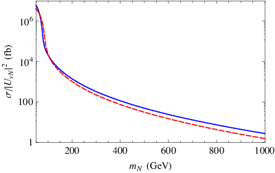
The equations for ${\cal L}^{\prime}$ above indicate that, although the heavy neutrinos $N_{R}$ do not directly have SM gauge interactions, through mixing they can interact with the SM gauge bosons. In particular, $N$ couples to $W$, $Z$, or $h$ at tree level, as can be seen from Eq. (23). Consequently, $N$ can be singly produced via the quark-level processes  $q\bar{q}^{\prime}\to W^{*}\to lN$  and  $q\bar{q}\to\bigl(h^{*},Z^{*}\bigr)\to\nu N$,  the former with a charged lepton $l$ in the final state being easier to observe. This implies that the LHC can, in principle, test the seesaw mechanism for $N$-mass values up to a TeV or so. Since all these $N$-production processes depend on the elements of $U_{\nu N}$, their size plays a crucial role as far as the testability of the seesaw mechanism is concerned. In Fig. 1, we show the cross section of  $pp\to lNX$  (solid curve) as a function of $m_{N}$ for $pp$ center-of-mass energy of  $\sqrt{s}=14$ TeV,  with the $U_{\nu N}$ element associated with the $WlN$ coupling set to unity. It is therefore interesting to examine how large the elements of $U_{\nu N}$ can be, taking into account constraints from existing experimental data, especially the light-neutrino masses. This we will do in the next section.

From Eq. (23), one can also extract the couplings of $N$ to SM particles in order to evaluate the rates of its decay modes. We have collected the formulas for the dominant modes in Appendix A, which each depend on the elements of $U_{\nu N}$. We will illustrate this dependence in the examples studied in the next section. Thus, once $N$ is discovered, one may gain additional information about neutrino mixing patterns by studying its individual decays and their branching ratios.

With only one generation and the requirement  $m_{N}\gg|m_{D}|$  for the $N$ mass, the light-neutrino mass is given by  $m_{\nu}=-m^{2}_{D}/m_{N}$  at leading order, which explains why the light-neutrino mass is much smaller than the mass of its charged-lepton partner. For one generation, the mixing between the light and heavy neutrinos has a magnitude of  $|U_{\nu N}|=|m_{D}/m_{N}|=(m_{\nu}/m_{N})^{1/2}$.  If $|U_{\nu N}|^{2}$ is large enough, the heavy neutrino $N$ may be produced at the LHC. However, with the light-neutrino mass constrained to be less than ${\cal O}$(1 eV), the size of $U_{\nu N}$ is bounded by  $10^{-5}(100{\rm\,GeV}/m_{N})^{1/2}$. Hence the mixing is extremely small, even with $m_{N}$ as low as 100 GeV. With such small mixing, it is not possible to produce enough number of heavy neutrinos to study its properties at the LHC. This may lead one to think naively that it is not possible to test type-I seesaw at the LHC. However, before drawing such a conclusion, one should make sure that with more than one generation the elements of $U_{\nu N}$ are always constrained to be as small as that with just one generation. We find that this is not generally true and that it is possible to have large enough $U_{\nu N}$ such that testing the seesaw mechanism at the LHC can be achieved.

With more than one generation, from Eqs. (19) and (20) we have the leading-order relation

Thus, if there is a nontrivial solution for $U_{\nu N}$ which makes the right-hand side vanish exactly, the elements of $U_{\nu N}$ can be large and evade the constrain  $|U_{\nu N}|^{2}=m_{\nu}/m_{N}$  in the one-generation case [10]. We will denote such a solution by $U_{0}$. Once $U_{0}$ is found, one should of course make sure that by adding a perturbation $U_{\delta}$ to $U_{0}$, so that  $U_{\nu N}=U_{0}+U_{\delta}$,  one can obtain the light-neutrino masses and mixing. As we discuss below, such solutions indeed exist. In the following we will work with three generations of light and heavy neutrinos.

Let us first consider what the rank of $U_{0}$ must be that can yield the right solutions. We find it convenient to work in the basis where $U_{0}$ is already diagonalized. In that case, $M_{N}$ generally is not diagonal. Since $M_{N}$ must be of rank three in order that the three heavy neutrinos have nonzero masses, the rank of $U_{0}$ must not be more than two, for otherwise the determinant of  $U_{0}M_{N}U_{0}^{\rm T}$  would not be zero in contradiction with the assumption  $U_{0}M_{N}U_{0}^{\rm T}=0$.  It turns out that $U_{0}$ of rank two is also problematic. Writing the diagonal form of $U_{0}$ as  $\hat{U}_{0}={\rm diag}(a,b,0)$,  we have

where $M_{ij}$ are the elements in $M_{N}$, which is symmetric. Since $M_{N}$ is of rank three, $M_{12,11,22}$ cannot all be simultaneously zero. This implies that, if we keep at least one of $a$ and $b$ nonzero, we have two types of nontrivial solutions with necessary and sufficient conditions: (1) $b=0$,  $M_{11}=0$  and  (2) $a=0$,  $M_{22}=0$.  We conclude that $U_{0}$ must be a rank-one matrix. This type of texture for the mass matrix can be made stable by imposing symmetries [10, 12].

Next we derive the general expression for $U_{0}$ which has rank one and satisfies

where  $\hat{M}_{N}={\rm diag}\bigl(M_{1},M_{2},M_{3}\bigr)$  as before. Without loss of generality, the diagonal form of $U_{0}$ can be chosen to be  $\hat{U}_{0}={\rm diag}(\hat{u},0,0)$,  with $\hat{u}$ being some constant. This is related to the nondiagonal $U_{0}$ by the biunitary transformation  $U_{0}=V^{\prime}\hat{U}_{0}V$,  where $V$ and $V^{\prime}$ are 3$\times$3 unitary matrices. As a consequence, $U_{0}$ and $\hat{U}_{0}$ share the same rank. Denoting the elements of $V^{(\prime)}$ by $V_{kl}^{(\prime)}$, we then arrive at

where $\kappa$ is a proportionality constant,  $\kappa a=\hat{u}V_{11}^{\prime}$,   $\kappa b=\hat{u}V_{21}^{\prime}$,  and  $\kappa c=\hat{u}V_{31}^{\prime}$.  Since this $U_{0}$ has to satisfy Eq. (29), we use the relation  $U_{0}=V^{\prime}\hat{U}_{0}V$  in the equation to find  $\hat{U}_{0}M_{N}\hat{U}_{0}^{\rm T}=0$,  where  $M_{N}=V\hat{M}_{N}V^{\rm T}$,  which is clearly symmetric and generally nondiagonal. As shown in the preceding paragraph, this implies that the (1,1) element of $M_{N}$ must vanish,  $M_{11}=0$,  which translates into

Thus, with $V_{11}$, $V_{12}$, and $V_{13}$ required to fulfill this condition, Eq. (II) has the desired expression for $U_{0}$ in terms of the parameters $a$, $b$, and $c$, which are to be fixed from experimental data.

To illustrate that one can find $U_{0}$ of the form in Eq. (II) that yields large light-heavy mixing while simultaneously satisfying constraints from various measurements, we find it convenient to consider specific examples. Accordingly, in the rest of this section we work in the basis in which $M_{N}$ is diagonal, writing

where we have regarded $m_{N}$ as representative of the mass scale of the heavy neutrinos, and so can take it to be the lightest of $M_{1,2,3}$. Then, choosing the appropriate $V_{11,12,13}$ in Eq. (II) to satisfy Eq. (34), as well as the unitarity relation  $|V_{11}|^{2}+|V_{12}|^{2}+|V_{13}|^{2}=1$,  and adjusting $\kappa$ in each instance, we obtain as examples for $U_{0}$

where we have factored out the diagonal matrix $\cal R$ in order to maintain the form of $U_{0}$ in cases where the heavy neutrinos are nondegenerate. In our numerical examples, we will use in particular only $U_{0}^{a}$ and $U_{0}^{d}$, although the other options would also be possible. We remark that it may sometimes be necessary to use trial and error in order to determine the right choice of $U_{0}$, with $a$, $b$, and $c$ being subject to experimental constraints that are relevant in specific circumstances.

We now show explicitly that one can find solutions for $U_{\nu N}$ which satisfy all experimental data on light neutrinos by adding a perturbation matrix $U_{\delta}$ given by

Since  $U_{0}\hat{M}_{N}U_{0}^{\rm T}=0$,  the light-neutrino mass matrix  $m_{\nu}=-U_{\nu N}\,\hat{M}_{N}\,U_{\nu N}^{\rm T}$  becomes

When trying to find solutions, one should keep in mind that $\delta_{ij}$ as perturbations should be much smaller than $a$, $b$, and $c$, while the size of  $(a,b,c)\delta_{kl}M_{i}$  is set by the light-neutrino masses. One can neglect the last term, $U_{\delta}M_{N}U^{\rm T}_{\delta}$, in Eq. (54) compared with the first two terms. In case the combination of the first two terms in Eq. (54) happens to vanish, one needs to keep the $U_{\delta}M_{N}U^{\rm T}_{\delta}$ term, the elements of $U_{\delta}$ now being of order $(m_{\nu}/m_{N})^{1/2}$.

References

• [1] C. Amsler et al. [Particle Data Group], Phys. Lett. B 667, 1 (2008) and 2009 partial update for the 2010 edition.
• [2] A. Zee, Phys. Lett. B 93, 389 (1980) [Erratum-ibid. B 95, 461 (1980)]; K.S. Babu, Phys. Lett. B 203, 132 (1988); E. Ma, Phys. Rev. Lett. 81, 1171 (1998) [arXiv:hep-ph/9805219]. A. Pilaftsis, Z. Phys. C 55, 275 (1992) [arXiv:hep-ph/9901206].
• [3] P. Minkowski, Phys. Lett. B 67, 421 (1977); T. Yanagida, in Proceedings of the Workshop on the Unified Theory and the Baryon Number in the Universe, edited by O. Sawada and A. Sugamoto (KEK, Tsukuba, 1979), p. 95; M. Gell-Mann, P. Ramond, and R. Slansky, in Supergravity, edited by P. van Nieuwenhuizen and D. Freedman (North-Holland, Amsterdam, 1979), p. 315; S.L. Glashow, in Proceedings of the 1979 Cargese Summer Institute on Quarks and Leptons, edited by M. Levy et al. (Plenum Press, New York, 1980), p. 687; R.N. Mohapatra and G. Senjanovic, Phys. Rev. Lett. 44, 912 (1980).
• [4] W. Konetschny and W. Kummer, Phys. Lett. B 70, 433 (1977); T.P. Cheng and L.F. Li, Phys. Rev. D 22, 2860 (1980); G. Lazarides, Q. Shafi, and C. Wetterich, Nucl. Phys. B 181, 287 (1981); J. Schechter and J.W.F. Valle, Phys. Rev. D 22, 2227 (1980); R.N. Mohapatra and G. Senjanovic, Phys. Rev. D 23, 165 (1981).
• [5] R. Foot, H. Lew, X.G. He, and G.C. Joshi, Z. Phys. C 44, 441 (1989).
• [6] T. Han and B. Zhang, Phys. Rev. Lett. 97, 171804 (2006) [arXiv:hep-ph/0604064]; B. Bajc, M. Nemevsek, and G. Senjanovic, Phys. Rev. D 76, 055011 (2007) [arXiv:hep-ph/0703080]; W. Chao, Z.G. Si, Z.Z. Xing, and S. Zhou, Phys. Lett. B 666, 451 (2008) [arXiv:0804.1265 [hep-ph]]; P. Fileviez Perez, T. Han, G.Y. Huang, T. Li, and K. Wang, Phys. Rev. D 78, 015018 (2008) [arXiv:0805.3536 [hep-ph]]; F. del Aguila and J.A. Aguilar-Saavedra, Phys. Lett. B 672, 158 (2009) [arXiv:0809.2096 [hep-ph]]; Z.Z. Xing, Int. J. Mod. Phys. A 24, 3286 (2009) [arXiv:0901.0209 [hep-ph]]; A. Atre, T. Han, S. Pascoli, and B. Zhang, JHEP 0905, 030 (2009) [arXiv:0901.3589 [hep-ph]]; N. Haba, S. Matsumoto, and K. Yoshioka, Phys. Lett. B 677 (2009) 291 [arXiv:0901.4596 [hep-ph]]; A. Arhrib, B. Bajc, D.K. Ghosh, T. Han, G.Y. Huang, I. Puljak, and G. Senjanovic, arXiv:0904.2390 [hep-ph]; P. Bandyopadhyay, S. Choubey, and M. Mitra, arXiv:0906.5330 [hep-ph]; W. Chao, Z.G. Si, Y.J. Zheng, and S. Zhou, arXiv:0907.0935 [hep-ph].
• [7] F. del Aguila, J. A. Aguilar-Saavedra and R. Pittau, JHEP 0710, 047 (2007) [arXiv:hep-ph/0703261].
• [8] R. Franceschini, T. Hambye, and A. Strumia, Phys. Rev. D 78, 033002 (2008) [arXiv:0805.1613 [hep-ph]].
• [9] F. del Aguila and J.A. Aguilar-Saavedra, Nucl. Phys. B 813, 22 (2009) [arXiv:0808.2468 [hep-ph]].
• [10] W. Buchmuller and D. Wyler, Phys. Lett. B 249, 458 (1990); W. Buchmuller and C. Greub, Nucl. Phys. B 363, 345 (1991); J. Gluza, Acta Phys. Polon. B 33, 1735 (2002) [arXiv:hep-ph/0201002]; G. Ingelman and J. Rathsman, Z. Phys. C 60, 243 (1993); A. Pilaftsis, Phys. Rev. Lett. 95, 081602 (2005) [arXiv:hep-ph/0408103]; A. Pilaftsis and T.E.J. Underwood, Phys. Rev. D 72, 113001 (2005) [arXiv:hep-ph/0506107]; J. Kersten and A.Y. Smirnov, Phys. Rev. D 76, 073005 (2007) [arXiv:0705.3221 [hep-ph]]; E. Ma, Mod. Phys. Lett. A 24, 2161 (2009) [arXiv:0904.1580 [hep-ph]]; Z.Z. Xing, Prog. Theor. Phys. Suppl. 180, 112 (2010) [arXiv:0905.3903 [hep-ph]].
• [11] Z. Maki, M. Nakagawa, and S. Sakata, Prog. Theor. Phys. 28, 870 (1962); B. Pontecorvo, Sov. Phys. JETP 26 (1968) 984 [Zh. Eksp. Teor. Fiz. 53 (1967) 1717].
• [12] X.G. He and E. Ma, Phys. Lett. B 683, 178 (2010) [arXiv:0907.2737 [hep-ph]].
• [13] T. Schwetz, M. Tortola, and J.W.F. Valle, New J. Phys. 10, 113011 (2008) [arXiv:0808.2016 [hep-ph]]; M. Maltoni and T. Schwetz, arXiv:0812.3161 [hep-ph]. Other recent fits are given by M.C. Gonzalez-Garcia and M. Maltoni, Phys. Rept. 460, 1 (2008) [arXiv:0704.1800 [hep-ph]]; G.L. Fogli et al., Phys. Rev. D 78, 033010 (2008) [arXiv:0805.2517 [hep-ph]].
• [14] P.F. Harrison, D.H. Perkins, and W.G. Scott, Phys. Lett. B 530, 167 (2002) [arXiv:hep-ph/0202074]; Z.Z. Xing, Phys. Lett. B 533, 85 (2002) [arXiv:hep-ph/0204049]; X.G. He and A. Zee, Phys. Lett. B 560, 87 (2003) [arXiv:hep-ph/0301092].
• [15] F. del Aguila, J. de Blas, and M. Perez-Victoria, Phys. Rev. D 78, 013010 (2008) [arXiv:0803.4008 [hep-ph]]; F. del Aguila, J.A. Aguilar-Saavedra, J. de Blas, and M. Perez-Victoria, arXiv:0806.1023 [hep-ph].
• [16] S. Antusch, C. Biggio, E. Fernandez-Martinez, M. B. Gavela and J. Lopez-Pavon, JHEP 0610, 084 (2006) [arXiv:hep-ph/0607020].
• [17] A. D. Martin, W. J. Stirling, R. S. Thorne and G. Watt, Eur. Phys. J. C 63, 189 (2009) [arXiv:0901.0002 [hep-ph]]; http://projects.hepforge.org/mstwpdf.
• [18] A. Abada, C. Biggio, F. Bonnet, M.B. Gavela, and T. Hambye, JHEP 0712, 061 (2007) [arXiv:0707.4058 [hep-ph]];
• [19] A. Abada, C. Biggio, F. Bonnet, M.B. Gavela, and T. Hambye, Phys. Rev. D 78, 033007 (2008) [arXiv:0803.0481 [hep-ph]].
• [20] X.G. He and S. Oh, JHEP 0909, 027 (2009) [arXiv:0902.4082 [hep-ph]];
• [21] A. Arhrib, R. Benbrik, and C.H. Chen, arXiv:0903.1553 [hep-ph].
• [22] T. Li and X.G. He, Phys. Rev. D 80, 093003 (2009) [arXiv:0907.4193 [hep-ph]].