UNIVERSITÀ DEGLI STUDI DI ROMA
“TOR VERGATA”
![[Uncaptioned image]](0907.1535v1/logoToV.png)
FACOLTÀ DI SCIENZE MATEMATICHE, FISICHE E NATURALI
Dipartimento di Fisica
Anomalies, and the MSSM
Tesi di Dottorato di Ricerca in Fisica
Antonio Racioppi
Relatore
Coordinatore del dottorato
Prof. Francesco Fucito
Prof. Piergiorgio Picozza
Ciclo XXI
Abstract
This Thesis reviews an extension of the MSSM by the addition of an anomalous abelian vector multiplet and contains some original results concerning the phenomenology of an anomalous .
The review part covers an introduction of the MSSM focusing on its main features, a discussion on the chiral anomalies and how to cancel them in the Standard Model and by the Green-Schwarz mechanism.
Then, the original results are presented. We build the Lagrangian for the Minimal Anomalous Extension of the MSSM where the anomalies are cancelled by the Green-Schwarz mechanism and the addition of Chern-Simons terms, stressing the main differences between our model and the MSSM. The advantage of this choice over the standard one is that it allows for arbitrary values of the quantum numbers of the extra . As a first step towards the study of hadron annihilations producing four leptons in the final state (a clean signal which might be studied at LHC) we then compute the decays and . We find that the largest values of the decay rate are GeV, while the expected number of events per year at LHC is at most of the order of 10. Then we compute the relic density predicted by our model with a new dark matter candidate, the axino, which is the LSP of the theory. We find agreement with experimental data admitting a bino-higgsino NLSP or a wino-like NLSP, almost degenerate in mass to the axino.
Acknowledgements
“There are many path to the top of the mountain.
But the view is always the same.”
Asian proverb
This Thesis work includes most of the research I have done during my PhD course at the University of Rome “Tor Vergata”. I wish to thank the Department of Physics and the Coordinator of the PhD program Prof. Piergiorgio Picozza for supporting my work. I spent several months of my PhD absent from Tor Vergata, at DAMTP in Cambridge, both of which I would like to thank for the hospitality and the resources they made available. I am also grateful to INFN for travelling support and to Marie Curie Research Training Network “Superstring Theory” for financial support.
First of all, my gratitude goes to my advisor Prof. Francesco Fucito, who first introduced and then continued to support me in a fascinating research field. Many thanks also to Prof. Massimo Bianchi, Dr. Andrea Lionetto, Prof. Yassen Stanev, Prof. Gianfranco Pradisi and Dr. Pascal Anastasopoulos for their kind assistance and support in Tor Vergata, to Prof. Michael Green for his hospitality in DAMTP and to Prof. Claudio Corianò for useful collaborations and discussions.
I am very grateful to all the friends I have been in touch with during these years. I would like to thank for their friendship: Andrea and Matteo (all started at the “campetto” and all will finish there). Valentina for her support and help in my troubles. Alberto, Ilaria and Maria Vittoria for their sustain and their visits. Elisa, Piero, Francesco and Laura for their support. “La Dottorandi” and in particular Simona, Francesco G., Giulia, Marine, Flavio, Andrea S., Maurizio and Andrea M.; a special thanks goes to Francesco S. for several intense Friday afternoons and his friendship. “The Lost Legacy”: Enrico, Regula and Alessandra. Gianluca and the YouTube searches. Paola and her verve. I also wish to thank Roberta, Michele and Sven for useful discussions and their friendship. I am grateful to UmbroTeam, Avis Frassati and Darwin College Team for giving me the possibility to play the best sport ever: basketball. Thanks to all of them, everywhere I was, I felt at home.
Last but not least. My deepest gratitude and love go to my parents and my brother for their support, encouragement and care throughout my studies and travels. Without them, nothing of this would be possible.
Chapter 1 Introduction
The Standard Model (SM) of particle physics has been confirmed to a great accuracy in many experiments. Despite the fact that the Higgs particle remains experimentally elusive, few scientists doubt that there will be major surprises in this direction. The whole scientific community, however, knows that the SM needs to be improved. Apart from the experimental discover of a tiny neutrino mass, there are also several theoretical issues that make physicists believe that the SM is only an effective manifestation of a more Fundamental Theory.
We know that a new framework must appear at the Planck scale ( GeV) where a theory of quantum gravity reveals. Since the ratio between this scale and the electroweak (EW) scale ( GeV) is huge, all quantum corrections will turn out to be many orders of magnitude greater then tree values. This is the so called hierarchy problem, related to fine-tuning and naturalness. Quantum corrections are power-law (usually quadratic) divergent which means that the highest energy physics is most important. More technically, the question is why the Higgs boson is so much lighter than the Planck scale. Indeed one would expect that the large quadratically divergent quantum contributions to the square of the Higgs boson mass would be inevitably make the mass huge, unless there is a fine-tuned cancellation between the quadratic radiative corrections and the bare mass.
Besides the hierarchy problem, there some unexplained features in cosmological observations. Measurements constraint the quantity of baryon matter, dark matter and dark energy in the universe revealing that the known particles make up only a small fraction of the total energy density of the universe. So particle physics must provide candidates for dark matter (DM) and dark energy and experiments to check the inherited models.
During the last years many ideas were used to overcome these problems. The most appealing theory is supersymmetry (SUSY), even if its historical motivation was to provide fermions in string theory. In 1981 it was proposed the Minimal Supersymmetric Standard Model (MSSM) i.e. the minimal extension of the SM which provides supersymmetry. SUSY pairs bosons with fermions, so each SM particle has a corresponding partner (unfortunately not discovered yet). SUSY removes the quadratic divergences of the radiative corrections to the Higgs mass. However, there is no understanding of why the Higgs mass is so small from the beginning ( problem). One of the most intriguing feature of the MSSM (and its extensions) is that it provides DM candidates with relic density compatible with experimental data. In fact, if -parity is conserved, the lightest supersymmetric particle of the MSSM is stable and makes it a good cold dark matter (CDM) particle.
As cited before, string theory was the framework where SUSY was born. Moreover it is also the most appealing candidate for a quantum theory of gravity. One of the prediction of string theory is the existence of anomalous U(1)’s. In standard theories the chiral anomalies are cancelled satisfying that the trace of the product of the gauge generators is zero. Instead in string theory this is not always possible, so the U(1)’s are anomalous, but the theory is still consistent and anomaly free, thanks to the Green-Schwarz (GS) mechanism. These anomalous gauge fields must be massive, otherwise we already discovered them, and the mass is acquired with the Stückelberg mechanism which was the first attempt to give a vector mass preserving gauge invariance, but phenomenologically ruled out in the SM. This procedure involves an axion-like scalar field, which plays also an important role in the GS mechanism for the anomaly cancellation. D-brane models contain several anomalous abelian factors living on each stack of branes. In the presence of these anomalous ’s, the GS couplings with the axions cancels mixed anomalies11 1 Irreducible anomalies are cancelled by the tadpole cancellation., and the Stückelberg mixing renders the “anomalous” gauge fields massive. The masses depend non-trivially on the internal volumes and on other moduli, allowing the physical masses of the anomalous gauge bosons to be much smaller than the string scale (even at a few TeV range). An important role is played by the so-called Generalized Chern-Simons terms (GCS) which are local gauge non-invariant terms. Indeed, these trilinear gauge bosons anomalous couplings are responsible for the cancellation of mixed anomalies between anomalous s and non anomalous factors ensuring the consistency of the theory.
In this Thesis, we are interested in anomaly related bosons and we present the results obtained in [1] and [2]. The theory is non-renormalizable since it has an energy cut-off related to the mass. More precisely, we study an extension of the MSSM by the addition of an abelian vector multiplet and we assume that generically all MSSM particles are charged with respect to the new . The anomalies are cancelled using the GS mechanism and the GCS terms, so the anomalous abelian boson becomes massive and behaves like a .
In approximately one year, the Large Hadron Collider (LHC) at CERN will start to operate at energies of order of 14 TeV in the center of mass (CM). Apart from the search for the Higgs boson, it will probably give us some answers about the parameter space of the physics beyond the SM, the eventual existence of new particles, such as the , and their nature.
This Thesis is organized as follows. In Chapter 2 we introduce the MSSM. We explain its main characteristics, focusing on the Renormalization Group Equations (RGEs) and the mass spectrum of the theory. In Chapter 3 we discuss the problem of the 1 loop chiral anomalies in field theory. We show how to cancel them with the standard procedure and with the GS mechanism, both in a standard and in a supersymmetric framework. In Chapter 4 we present our model. We discuss the Lagrangian and the differences between our theory and the MSSM. In Chapter 5 we analyze some phenomenological consequences of our model such as the anomalous decays and the prediction of the relic density with a new dark matter candidate. In Chapter 6 we summarize the conclusions and the results of our work. Finally in the Appendix we give further details of the computations omitted in the main body of the Thesis.
Chapter 2 Overview of the MSSM
Supersymmetry is the only possible non trivial unification of internal and space-time symmetries compatible with quantum field theory. It emerges naturally in string theory but it can be introduced apart of it. A SUSY transformation turns a bosonic state into a fermionic state increasing its spin by , and viceversa. The single particle states of a supersymmetric theory fall into irreducible representations of the SUSY algebra, called supermultiplets which, in turn can be organized into superfield. Each supermultiplet contains both fermion and boson states that are superpartners of each other. One may show that no particle of the SM can be the superpartner of another, so SUSY predicts a list of new particles, none of which has been discovered yet. In reason of this, superpartners cannot be mass degenerate and so SUSY must be a broken symmetry. There are several ways to introduce a breaking of SUSY, however the simplest way is to explicit break it adding ad hoc mass terms. This is done in the MSSM. The following treatment of the MSSM is based on the works of Martin [3] and Derendinger [4].
2.1 The superpotential
In a renormalizable supersymmetric field theory, the interactions and masses of all particles are determined just by their gauge transformation properties and by the superpotential . is an analytic function of the complex chiral superfield . The gauge quantum numbers and mass dimensions of a chiral superfield are given by these of its scalar component. In the superfield formulation we write the superpotential as
| (2.1) |
Given the supermultiplet content of the theory, the form of the superpotential is guided by the requirement of gauge invariance, so only a subset of the parameters and are allowed to be different from zero. The entries of the mass matrix can be non zero only for and such that the superfield and have gauge transformation conjugates of each other. Similarly for the Yukawa couplings . The interactions implied by the superpotential were shown in Fig. 2.1-2.2.
††feynman-diagram: (Feynman diagram, (x6) ††feynman-diagram: (Feynman diagram, (x6) ††feynman-diagram: (Feynman diagram, (x6)
(a) (b) (c)
††feynman-diagram: (Feynman diagram, (x6) ††feynman-diagram: (Feynman diagram, (x6)
(a) (b)
††feynman-diagram: (Feynman diagram, (x6) ††feynman-diagram: (Feynman diagram, (x6) ††feynman-diagram: (Feynman diagram, (x6)
(c) (d) (e)
| Supermultiplet | Gauge Representation | ||||
|---|---|---|---|---|---|
| Superfield | Spin | Spin | |||
| Supermultiplet | Gauge Representation | ||||
|---|---|---|---|---|---|
| Superfield | Spin | Spin | |||
| or | 0 | ||||
| or | 0 | ||||
| or | 0 | ||||
††feynman-diagram: (Feynman diagram, (x6) ††feynman-diagram: (Feynman diagram, (x6) ††feynman-diagram: (Feynman diagram, (x6)
(a) (b) (c)
††feynman-diagram: (Feynman diagram, (x6) ††feynman-diagram: (Feynman diagram, (x6) ††feynman-diagram: (Feynman diagram, (x6)
(d) (e) (f)
††feynman-diagram: (Feynman diagram, (x6) ††feynman-diagram: (Feynman diagram, (x6) ††feynman-diagram: (Feynman diagram, (x6)
(g) (h) (i)
The particle content of the MSSM is given in Table 2.1-2.2. The superpotential for the MSSM is
| (2.2) |
where the indices run over the three families. For the complete Langrangian of the MSSM see Appendix B.1.
All of the gauge indices in eq. (2.2) are suppressed. The “ term”, as it is usually called, can be written out as , where is used to tie together weak isospin indices in a gauge-invariant way. Similarly for the terms , and .
The term in eq. (2.2) is the supersymmetric version of the Higgs boson mass in the SM. It is unique, since terms or are forbidden in the superpotential, because it must be analytic in the chiral superfields. We can also see from the form of eq. (2.2) why both and are needed in order to give Yukawa couplings, and thus masses, to all of the quarks and leptons. Since the superpotential must be analytic, for instance the Yukawa terms cannot be replaced by something like . So we need both and , even without invoking the argument based on anomaly cancellation (as we will see in Section 3.2).
Since the top quark, bottom quark and tau lepton are the heaviest fermions in SM, it is common to use the approximation that only the third (3,3) component of , and are important
| (2.3) |
In this limit the MSSM superpotential reads in components
| (2.4) | |||||
where , , , , , and . The minus sign inside the parentheses appear because of the use of to tie up internal indices. These minus signs were chosen so that terms proportional to , and have positive signs when they become the top, bottom and tau masses.
Since the Yukawa interactions in a general supersymmetric theory must be completely symmetric under interchange of , we know that , and imply not only Higgs-quark-quark and Higgs-lepton-lepton couplings as in the SM, but also squark-higgsino-quark and slepton-higgsino-lepton interactions.
There are also scalar quartic interactions with strength proportional to the square of Yukawa couplings. The existence of all the quark and lepton Yukawa couplings in the superpotential (2.2) leads also to the following scalar quartic couplings: (squark)4, (slepton)4, (squark)2(slepton)2, (squark)2(Higgs)2 and (slepton)2(Higgs)2. However, the dimensionless interactions determined by the superpotential are usually not the most important ones of direct interest for phenomenology. This is because the Yukawa couplings are already known to be very small, except for those of the third family (top, bottom, tau). Instead, production and decay processes for superpartners in the MSSM are typically dominated by the supersymmetric interactions of gauge-coupling strength. The couplings of the Standard Model gauge bosons (, , and gluons) to the MSSM particles are determined completely by the gauge invariance of the kinetic terms in the Lagrangian. The gauginos also couple to (squark, quark) and (slepton, lepton) and (Higgs, higgsino) pairs as illustrated in the general case in Fig. 2.3. For instance, each of the squark-quark-gluino couplings is given by where are the matrix generators for .
The dimensionful couplings in the supersymmetric part of the MSSM Lagrangian are all dependent on . From eq. (2.2), we get the higgsino fermion mass terms
| (2.5) |
as well as Higgs squared-mass terms in the scalar potential
| (2.6) |
Since eq. (2.6) positive definite, we cannot understand electroweak symmetry breaking (EWSB) without including a negative supersymmetry-breaking squared-mass soft term for the Higgs scalars (see Section 2.4.1). Moreover we expect that should be roughly of order or GeV, not so far from the electroweak scale. But why is so small compared to ? Why should it be roughly of the same order as ? The scalar potential of the MSSM seems to depend on two distinct dimensionful parameters, namely the supersymmetry-preserving mass and the supersymmetry-breaking soft mass terms. The observed value for the electroweak breaking scale suggests, both of these should be within an order of magnitude or so of 100 GeV. This puzzle is called “the problem”. Several different solutions to the problem have been proposed, but they all work in roughly the same way11 1 Some other attractive solutions are proposed in [5]-[7].; the term is absent at tree-level before symmetry breaking, and then it arises from the VEV(s) of some new field(s). These VEVs are determined by minimizing a potential that depends on soft terms. Thus, the value of the effective parameter is related to supersymmetry breaking. From the point of view of the MSSM, however, we can just treat as an independent parameter.
Finally, the -term and the Yukawa couplings in the superpotential eq. (2.2) combine to yield (scalar)3 couplings of the form
| (2.7) | |||||
2.2 Soft supersymmetry breaking
A realistic phenomenological model must contain SUSY breaking. From a theoretical point of view we expect that SUSY is an exact symmetry which is spontaneously broken. Many models have been proposed but we do not discuss them because is beyond our scope. From a practical perspective it is sufficient to parametrize our ignorance introducing extra terms that break explicitly SUSY. However this breaking should be soft because we do not want to lose the main properties of a SUSY theory (see Chapter 1 and [3]). As illustrated in [4] the one loop divergent contributions to the scalar potential are given by
| (2.8) |
where is the energy cut-off and is the mass matrix of the theory. As it is well known a SUSY theory is free of quadratic divergences, in fact , so the soft breaking terms must be such that this property still holds.
††feynman-diagram: (Feynman diagram, (x6) ††feynman-diagram: (Feynman diagram, (x6) ††feynman-diagram: (Feynman diagram, (x6) ††feynman-diagram: (Feynman diagram, (x6)
(a) (b) (c) (d)
The possible soft supersymmetry breaking of a general renormalizable theory are
| (2.9) |
They are gaugino masses for each gauge group, scalar squared mass terms and and trilinear scalar coupling . There are no mass terms for the chiral supermultiplet fermions, like , because in general they are not soft22 2 In Section 4.1.2 we will see a case in which is possible to have such a term.. The Lagrangian breaks SUSY since it involves only scalars and gauginos and not their respective superpartners. The gaugino masses are always allowed by gauge symmetry. The terms are allowed for such that transform in complex conjugate representations under all gauge groups. This is obviously true when , so every scalar can acquire mass in this way. The remaining soft terms are restricted by the symmetries. Because the and have the same form as and , they will be allowed if and only if there is a corresponding superpotential term in the Lagrangian. The corresponding Feynman diagrams are given in Fig. 2.4.
Applying what we have shown to the MSSM, we get that
| (2.10) | |||||
We see soft mass terms for the gluinos , the winos and the bino . Then we have the (scalar)3 couplings, which are in one to one correspondence with the Yukawa couplings of the superpotential and the sleptons and squarks masses. As usual we suppressed the gauge indices. Finally we have the soft terms that contributes to the Higgs potential, , and .
The above introduces many new parameters which are absent in the ordinary SM. A careful count [8] shows that there are 105 masses, phases and mixing angles in the MSSM Lagrangian that cannot be rotated away by some redefinition of the basis of quark and lepton supermultiplets. However there are experimental flavor mixing and CP violation data which limit this number [9]. All of these potentially dangerous effects can be avoided assuming that supersymmetry breaking is “universal”. In particular we can suppose that the squark and slepton masses are flavor-blind, then
| (2.11) |
If so, then all sfermions mixing angles are trivial. Therefore MSSM contributions to FCNC processes will be very small up to mixing induced by , and . Making the further assumption that these couplings are proportional to the respective Yukawa coupling,
| (2.12) |
will ensure that only the sfermions of the third family can have large (scalar)3 couplings. Finally, to avoid large CP-violation effects it is usually assumed that soft terms do not introduce new complex phases. This is automatic for the Higgses and the sfermions if eq. (2.11) is true. We can also fix the and parameters to be real, rotating the phase of supermultiplets. Assuming also that the in eq. (2.12) and the gaugino soft masses are real, then the only CP-violating phase in the theory will be the ordinary CKM phase of the SM.
2.3 RGE
In this section we list the result for the RGEs in the MSSM. For a method of computation see for instance [4].
The 1 loop RG equations for the gauge couplings are
| (2.13) |
where with the RG scale, , and . The normalization of is chosen to agree with Grand Unification Theories (GUTs) like or . The quantities turn out to have their reciprocals that run linearly with the RG scale
| (2.14) |
In Fig. 2.5 is plotted the RG evolution of the . Unlike the SM, which has a very rough unification, MSSM has a very “precise” unification at the scale GeV. This can be an accident, but it may also be taken as a hint toward SUSY GUT or superstring models.

Next we consider the 1 loop RGEs of the parameters in the superpotential. Considering the third family approximation (2.3) we get the following equations for the Yukawa couplings
| (2.15) | |||||
| (2.16) | |||||
| (2.17) |
while the RGE for the term is
| (2.18) |
The one-loop RG equations for the three gaugino mass parameters in the MSSM are determined by the same quantities that appear in the gauge coupling RG eqs. (2.13)
| (2.19) |
for . It is easy to check that the three ratios are each constant (RG scale independent) at 1 loop order. Since the gauge couplings unify at GeV, it is a natural assumption that the gaugino masses also unify near that scale, with a value . If so, then it follows that
| (2.20) |
at any RG scale, up to small two-loop effects. Here is the unified gauge coupling at .
Then we consider the 1-loop RG equations for the soft parameters connected to the superpotential. Using the third family approximation (2.3) we can write at any RG scale
| (2.21) |
which defines the running parameters , and . In this approximation the RGEs for the trilinear soft couplings are
| (2.22) | |||||
| (2.23) | |||||
| (2.24) | |||||
while the RGE for the parameter is
| (2.25) | |||||
The -function for each of these soft parameters is not proportional to the parameter itself, because couplings which break supersymmetry are not protected by supersymmetric non-renormalization theorems.
Next let us consider the RG equations for the scalar masses in the MSSM. In the approximation of eqs. (2.3) and (2.21), the scalar masses satisfy boundary conditions like eq. (2.11) at an input RG scale, so when renormalized to any other RG scale, they will stay almost diagonal,
| (2.26) |
The first and second family sfermions remain very nearly degenerate
| (2.27) |
but the third-family sfermions have larger Yukawa couplings and so their squared masses get renormalized differently. The one-loop RGEs for the first and second family squark and slepton squared masses are
| (2.28) |
for each scalar , where runs over the three gauge groups , and , are the quadratic Casimir invariants and are the corresponding running gaugino masses. Also,
| (2.29) |
The right-hand side of eq. (2.28) is negative33 3 The contributions proportional to is zero in mSUGRA models., so the scalar squared-mass parameters grow as they are RG-evolved from the input scale down to the EW scale. The scalars masses will obtain large positive contributions at the electroweak scale, because of the effects of the gaugino masses.
The RG equations for the remaining scalars, Higgs and third family sfermions, also get contributions from the large Yukawa () and soft () couplings. It is useful to define the following quantities
| (2.30) | |||||
| (2.31) | |||||
| (2.32) |
In terms of these quantities, the RGEs for the soft Higgs squared-masses are
| (2.33) | |||||
| (2.34) |
while the RG equations for the third family sfermions mass parameters are
| (2.35) | |||||
| (2.36) | |||||
| (2.37) | |||||
| (2.38) | |||||
| (2.39) |
An examination of eq. (2.22)-(2.25), (2.28), and (2.33)-(2.39) reveals that if the gaugino masses , , and are non-zero at the input scale, then all of the other soft terms will be generated too. On the other hand, if the gaugino masses vanished at tree-level, then they would not get any contributions to their masses at the one-loop order; in that case the gauginos would be extremely light and the model would not be phenomenologically acceptable.
2.4 Mass spectrum
2.4.1 Electroweak symmetry breaking
In the MSSM, the description of electroweak symmetry breaking is slightly complicated by the fact that there are two complex Higgs doublets and rather than just one in the ordinary SM. The classical scalar potential for the Higgs sector in the MSSM is given by
| (2.40) | |||||
The terms proportional to come from -terms while the terms proportional to and are the -term contributions. Finally, the terms proportional to , and are coming from the soft breaking Lagrangian (2.10). The full scalar potential of the theory also includes many terms involving the sparticle fields which we can ignore here, since they do not get VEVs because they have large positive squared masses.
We now have to demand that the minimum of this potential should give a correct electroweak symmetry breaking . It is easy to see that in the minimum we have . This is good, because it means that at the minimum of the potential electromagnetism remains unbroken, since the charged components of the cannot get VEVs. After setting , we are left to consider the scalar potential
| (2.41) | |||||
The only term in this potential that depends on the phases of the fields is the -term. Therefore, redefining the phase of or we can absorb any phase in , so we take to be real and positive. To have a bounded from below potential and to avoid the possibility to have in the minimum, the parameters in the potential must obey the following constraints
| (2.42) | |||||
| (2.43) |
Having established the conditions necessary for and to get non-zero VEVs, we can now require that they give a correct EW phenomenology. Let us write
| (2.44) |
These VEVs are related to the known mass of the boson and the gauge couplings (see eq. (2.84))
| (2.45) |
The ratio of the VEVs is usually written as
| (2.46) |
The value of is not fixed by experiments, but it depends on the Lagrangian parameters of the MSSM in a calculable way. Now we can write down the conditions for minimizing the potential
| (2.47) | |||
| (2.48) |
Using , , and as input parameters, we can solve these two equations to give the values for and
| (2.49) | |||||
| (2.50) |
In the following subsections we will treat the mass spectrum for each particle sector of the theory at tree level.ù
2.4.2 Higgs Bosons
The Higgs scalar fields in the MSSM consist of two complex -doublet, so eight real, scalar degrees of freedom. When the electroweak symmetry is broken, three of them are the would-be Nambu-Goldstone (NG) bosons , , which become the longitudinal modes of the and massive vector bosons. The remaining five Higgs scalar mass eigenstates consist of two CP-even neutral scalars and , one CP-odd neutral scalar , and a charge scalar and its conjugate charge scalar .44 4 Here we define and . Also, by convention, is lighter than . The gauge-eigenstate fields can be expressed in terms of the mass eigenstate fields as
where the orthogonal rotation matrices
| (2.65) |
are chosen to diagonalize quadratic part of the potential
| (2.66) | |||||
The mass eigenvalues are given by
| (2.67) | |||||
| (2.68) | |||||
| (2.69) | |||||
| (2.70) |
The mixing angle is determined by
| (2.71) |
and is traditionally chosen to be negative, so (provided ).
The masses of , and can in principle be arbitrarily large since they all grow with . In contrast, the mass of is bounded above. From eq. (2.68), one finds at tree-level [10]
| (2.72) |
If this inequality were robust, we would have discovered the lightest Higgs boson at LEP2. In fact the tree level formula (2.68) is subject to drastic quantum corrections and it is possible to show that can exceed the LEP bounds. Assuming that none of the sfermions masses exceed 1 TeV and that all the couplings in the model remain perturbative up the GUT scale, we get [11]
| (2.73) |
However the previous bound is weakened if we relax one of the previous assumptions.
2.4.3 Vector Bosons
The gauge bosons in the MSSM get masses in the same way of the SM with the identification . We recall very briefly the Lagrangian
| (2.79) | |||||
where the eigenstates are (the Weinberg angle is defined by )
| (2.80) | |||||
| (2.81) | |||||
| (2.82) |
and their corresponding eigenvalues are
| (2.83) | |||||
| (2.84) | |||||
| (2.85) |
The corresponding coupling constants are
| (2.86) | |||||
| (2.87) | |||||
| (2.88) |
Exactly the same results of SM.
2.4.4 Neutralinos and Charginos
The higgsinos and electroweak gauginos mix with each other because of the effects of EWSB. The neutral higgsinos ( and ) and the neutral gauginos (, ) combine to form four mass eigenstates called neutralinos (). The charged higgsinos ( and ) and winos ( and ) mix to form two mass eigenstates with charge called charginos ().55 5 Other common notations use or for neutralinos, and or for charginos. By convention, these are labelled in ascending order, so that and .
With the basis , the neutralino mass part of the Lagrangian is
| (2.89) |
where is the following matrix
| (2.90) |
where the lower dots denote the obvious terms under symmetrization. The entries and are the soft gaugino masses in (2.10), while the entries are the supersymmetric higgsino mass terms in (2.2). The terms proportional to are the result of Higgs-higgsino-gaugino couplings (see Fig. 2.3 g,h), with the Higgs replaced by their VEVs.
The parameters , , and in the equations above can have arbitrary complex phases. A redefinition of the phases of and permit us to choose and both real and positive. The phase of within that convention is then really a physical parameter and cannot be rotated away. However, if is not real, then there can be potentially disastrous CP-violating effects in low-energy physics, so it is usual to assume that is real in the same set of phase conventions that make , , , and real and positive. The sign of is still undetermined by this constraint.
There is a not-unlikely limit in which EWSB is a small perturbation inside
| (2.91) |
In this case the neutralino eigenstates are very nearly a “bino-like” , a “wino-like” and “higgsino-like” , with masses
| (2.92) | |||||
| (2.93) | |||||
| (2.94) | |||||
| (2.95) |
where and are respectively the cosine and sine of the Weinberg angle and is the sign of the parameter. The neutralino labels should be rearranged depending on the numerical values of the parameters; in particular the above labelling is a common situation in mSUGRA models.
The chargino spectrum can be treated in a similar way. In the gauge-eigenstate basis , the chargino mass terms are
| (2.96) |
where, in block form,
| (2.97) |
Since these are only 22 matrices, it is easy to find the mass eigenvalues
| (2.98) | |||||
In the limit of eq. (2.91), the charginos consist of a wino-like and a higgsino-like , with masses
| (2.99) | |||||
| (2.100) |
The labelling is given in the same way as the neutralino case. Amusingly, is nearly degenerate with in the approximation shown, but it is not an exact result. Similarly the higgsino-like fermions , and have masses close to .
2.4.5 Gluinos
The gluino is a color octet fermion, it cannot mix with any other particle in the MSSM. Because it is not involved in EWSB, the only source of its mass is the soft parameter . In mSUGRA models this soft mass is related to the other soft gaugino masses, giving the rough prediction
| (2.101) |
near the TeV scale. Then it is reasonable to suppose that the gluino is much heavier than the lighter neutralinos and charginos.
2.4.6 Sfermions
A priori, any scalars with the same electric charge, -parity66 6 See Subsection 2.5., and color quantum numbers can mix with each other. This means that in general, the mass eigenstates of the squarks and sleptons of the MSSM should be obtained by diagonalizing three squared-mass matrices for up-type squarks (, , , , , ), down-type squarks (, , , , , ), and charged sleptons (, , , , , ), and one matrix for sneutrinos (, , ). However with the assumptions (2.3), (2.21) and the result (2.27) we have that the first and second families are almost eigenstates while we can have the previous mixings only for the third family sfermions. So the masses for the squarks and sleptons of the first two families are
| (2.102) | |||||
| (2.103) | |||||
| (2.104) | |||||
| (2.105) | |||||
| (2.106) | |||||
| (2.107) | |||||
| (2.108) |
where . The first and most important contribution are the soft masses given in (2.11) while the second (and the third) one comes from terms. We can see a degeneracy between the sfermions with the same charges. Instead the mass matrix for the third family squarks is
| (2.109) |
where
| (2.110) |
We can see that the diagonal entries are similar contributions as the first two families plus the one coming from Yukawa couplings which now are not negligible. Finally the mass terms for the tau sleptons
| (2.111) |
and their corresponding sneutrino
| (2.112) |
As in the previous case the diagonal entries for (2.111) have the similar first(second) family contribution plus the Yukawa correction.
2.5 parity
The superpotential (2.2) is minimal in the sense that it is sufficient to produce a phenomenologically viable model. However we can write other terms (gauge-invariant, renormalizable and analytic in the chiral superfields) which are not included in the MSSM since they do not respect either baryon number () or total lepton number (). These terms are
| (2.113) | |||||
| (2.114) |
where runs over the three families. The baryon and lepton number assignment are the usual ones: for , for and for all others; for , for , and for all others. So the terms in eq. (2.113) violate total lepton number by 1 unit (as well as the individual lepton flavors) and those in eq. (2.114) violate baryon number by 1 unit.
The possible existence of such terms might seem rather disturbing, since corresponding - and -violating processes (for example the proton decay) have not been seen experimentally. One could simply try to postulate and conservation in the MSSM by adding a new symmetry, which has the effect of eliminating the possibility of and violating terms in the renormalizable superpotential, while allowing the good terms in eq. (2.2). This new symmetry is called “-parity” [12] and it is defined as
| (2.115) |
where is the spin of the particle. Therefore particles within the same supermultiplet do not have the same -parity77 7 In general, symmetries with the property that fields within the same supermultiplet have different transformations are called symmetries; they do not commute with supersymmetry.. The -parity assignment is very useful for phenomenology because all of the SM particles and the Higgs bosons have , while all of the squarks, sleptons, gauginos, and higgsinos have . The -parity odd particles are known as “sparticles” (“supersymmetric particles”), and they are distinguished by a tilde (see Tables 2.1 and 2.2). -parity conservation implies that there can be no mixing between the and the particles. Furthermore, every interaction vertex in the theory contains an even number of sparticles. This has three extremely important phenomenological consequences:
- i.
The lightest particle, called the LSP (“lightest supersymmetric particle”), must be absolutely stable. If the LSP is electrically neutral, it interacts only weakly with ordinary matter, and it can be an attractive candidate [13] for the non-baryonic dark matter.
- ii.
Each sparticle other than the LSP must decay into a state that contains an odd number of sparticles.
- iii.
In collider experiments, sparticles can only be produced in even numbers.
We define the MSSM to conserve -parity. This decision seems to be well-motivated phenomenologically by proton decay constraints, but it might appear somewhat artificial from a theoretical point of view. One attractive solution could occur if BL is a continuous gauge symmetry because it forbids the renormalizable terms that violate B and L [14, 15]. However, the must be spontaneously broken at some very high energy scale, because there is no corresponding massless vector boson. Moreover, if it is only broken by scalar VEVs (or other order parameters) that carry even integer values of BL, then will automatically survive as an exactly conserved discrete remnant subgroup [15]. is called “matter-parity” and can be treated in a similar way as . A variety of extensions of the MSSM in which exact -parity conservation is guaranteed in just this way have been proposed (see for example [15, 16]).
Chapter 3 Anomalies
A theory is anomalous if at the quantum (loop) level a classical symmetry of the Lagrangian is no longer conserved. If is an anomalous global group the quantum theory remains consistent (for example ). Instead, if is an anomalous gauge group, the quantum theory becomes inconsistent, so the condition of anomaly cancellation may be used as a constraint on the physical gauge theories. The first studies on anomalies emerged in trying to understand the decay rate of the already cited neutral pion, in the form of an anomaly that violates some global symmetry of the strong interactions. In 1969 the source of this anomaly was traced by Bell and Jackiw [17] to the violation of chiral symmetry by the regulator that is needed in order to derive consequences of the conservation of the neutral axial vector current for one loop Feynman diagrams. Their result was confirmed and generalized by Adler [18]. After 10 years, Fujikawa [19] showed that the chiral symmetry breaking anomaly enters only in the measure used to define the path integral over fermion fields. The following treatment of anomalies is based on Chapter 22 of the book by Weinberg [20] and Chapter 6 of the book by Cheng and Li [21]. We will discuss the anomalies only from a Feynman diagram point of view, leaving the Fujikawa argument to the reader (for a review see also Section 22.2 of [20])
3.1 Triangular Anomaly
Consider a chiral gauge theory given by a certain number of massless left(right) Weyl fermions charged under two gauge fields11 1 The extension to a larger number of gauge fields and to a non abelian case can be treated in a similar way. and
| (3.1) |
where are the left(right) Weyl fermions in the model, and
| (3.2) |
is the covariant derivative. We can express the Lagrangian in terms of the Dirac spinors obtaining
| (3.3) | |||||
where the vectorial (V) and axial (A) couplings are given by
| (3.4) | |||||
| (3.5) |
with . For the conventions on the sigma matrices and the properties of gamma matrices see Appendix A.
We may be interested in computing the one loop amplitude and the corresponding Ward Identities (WIs) for an incoming and two outgoing . The Feynman diagrams involved are depicted in Fig. 3.1. The Feynman rules for the interacting vertices are given in Appendix C.1. We can split the amplitude in four contributions: AVV, VAV, VVA and AAA
| (3.6) | |||||
where
| (3.7) | |||||
| (3.8) | |||||
| (3.9) | |||||
| (3.10) | |||||
††feynman-diagram: (Feynman diagram, (x6) + ††feynman-diagram: (Feynman diagram, (x6)
The notation means that we have an axial vertex () on the line, a vectorial vertex () on the line and a vectorial vertex () on the line. Analogously for the other ’s.
Consider the first contribution. We have
| (3.11) | |||
The integral is superficially divergent so it is not uniquely defined (see Appendix D.1). Eq. 3.11 implies a particular choice for the assignment of the internal momentum : the fermion line between the two lines carries momentum . We could have chosen a different assignment of it so that this fermion line carries , where is some arbitrary combination of and
| (3.12) |
The fact that the integral is linearly divergent implies that has an ambiguity in its definition by an amount
| (3.13) | |||||
Applying the result (D.6), we have
| (3.14) | |||||
where we used
| (3.15) |
Since is related to by the exchanges and , we have from eq. (3.12), (3.13) and (3.14)
| (3.16) |
Thus the definition of has an ambiguity parametrized by
| (3.17) |
Now we are going to show what is the relation between the ambiguity in the amplitude and the WIs. In quantum field theory, the WIs are identities between correlation functions that follows from the global or gauged symmetries of the theory, and which remains valid after renormalization. The WIs are a quantum version of the classical Noether’s theorem, and any symmetries in a quantum field theory can lead to an equation of motion for correlation functions. We can express them using Feynman amplitude in momentum space or by the path integral formulation. We will usually adopt the first formulation. The WIs for massless gauge fields can be written in the diagrammatic form showed in Fig. 3.2.
††feynman-diagram: (Feynman diagram, (x4)
We start with the incoming momentum . Using eq. (3.17), we have
| (3.18) |
and we focus on the first contribution
| (3.19) |
where the first term is
| (3.20) | |||||
while the second one is with the exchange
| (3.21) |
We rearrange the computation grouping the integrals with only a dependence or only a dependence. So
| (3.22) |
where
| (3.23) | |||||
| (3.24) |
Using the result (D.6) we get
| (3.25) | |||||
In the last line we used eq. (3.15) and the last identity follows simply by the definition (3.24). Then using eq. (3.18), (3.19), (3.22) and (3.25) we find
| (3.26) |
In a similar way we can compute the WIs for the and momenta, obtaining
| (3.27) | |||||
| (3.28) |
A similar analysis can be done for the other VAV, VVA and AAA amplitudes in eq. (3.8)-(3.10). So the amplitude has the following WIs
| (3.29) | |||||
| (3.30) | |||||
| (3.31) |
with
| (3.32) | |||||
where we used eq. (3.4) and (3.5). As we can see from eq. (3.29), (3.30) and (3.31), there is no choice of that cancels simultaneously all the WIs and preserves gauge invariance, recovering the result depicted in Fig. 3.2. The same problem will arise in the computation of the , , and triangles. This is the “triangular (or chiral) anomaly”. The classical gauge invariance is broken by the triangular fermionic loop making the theory anomalous. Obviously, to have a physical gauge theory we must cancel this anomaly and the standard (and simplest) way is to cancel the overall sum of charges in the WIs. In other words the theory will be anomaly free if the charges satisfy the following constraints
| (3.33) | |||||
| (3.34) | |||||
| (3.35) | |||||
| (3.36) |
Depending on the symmetries of the problem, there are cases in which there is a preferential choice for the parameter. The most common values are (see eq. (3.29), (3.30) and (3.31):
- •
, for which all the anomaly is concentrated in the vertex .
- •
, for which the anomaly is equally distributed among the three vertices (to be used when we have three identical external vectors).
The extension to non abelian theories goes in the same way. The overall charge factor will become
| (3.37) |
where are the generators of the three external gauge fields. In some theories the condition of anomaly cancellation will fix completely the charge content of the model. This is the case for the SM (see for instance Section 22.4 of [20]).
3.2 Anomaly cancellation. SM and MSSM
The SM gauge group is and its fermionic content is displayed in Table 3.1
Now we check that vanishes for all the generators of the SM gauge group. We need only to consider those combinations of generators for which the product of , and is neutral under , since obviously vanishes for all the others. We can make invariants out of either zero, two or three or generators and any number of generators. We will use the following notation. is the hypercharge and , are the generators of the and algebras respectively. In our notation . So we need to check the following cases
- •
. Here vanishes because the left-handed fermions furnish a representation of which is real. In other words, for each quark, the contribution is cancelled exactly by the corresponding contribution.
- •
. Here the anomaly is
(3.38) - •
. There is no anomaly here because only has real or pseudoreal representations.
- •
. There the anomaly is
(3.39) - •
. There the anomaly is
(3.40)
There is one more anomaly that needs to be evaluated. All the fermions interact also with gravity. We can have anomalies different from zero generated by the fermionic with an incoming gauge vector a two outgoing gravitons. This anomaly is proportional to the trace of the gauge generator involved in the diagram. For and there is no problem because the generator are traceless, so we need to check only the hypercharge. We have
| (3.41) |
so there are no gravitational anomalies in the SM.
The same happens for the MSSM. With respect to the SM now we have two new fermions that are involved in the anomalies, the higgsinos. As we have just seen, the SM fermions contribution is zero, so the only relevant contribution comes from the supersymmetric sector. However and have opposite charge assignment (see Table 2.1) so that the higgsino contribution is zero. The final result is an anomaly free model.
3.3 Anomaly cancellation. Green-Schwarz mechanism
3.3.1 Introduction
Before introducing the GS mechanism, we give a generalization of the chiral anomalies in even dimensions . In any even dimensions (and only in even dimensions) one can define a chirality matrix that anticommutes with all matrices , (compare with eq. (A.6)). One can then have massless fermions that are chiral, i.e. either left-handed or right-handed. As in Section 3.1, the anomalies can again be traced to the presence of the chirality matrix (i.e. axial coupling) in the interaction vertices between fermions and vectors. In dimensions the traces involving will lead to an , and again the WIs on the amplitude with external vector, , must involve this tensor. Since this -tensor is completely antisymmetric in all its indices, to get a non vanishing expression we need at least indices and different independent momenta. Hence the minimal value for is . It follows that in dimensions the anomaly first manifests itself in the loop amplitude with external vectors. In four dimensions this corresponds to the fermionic triangle loop. For further details and general properties of the anomalies, we remand for instance to [22].
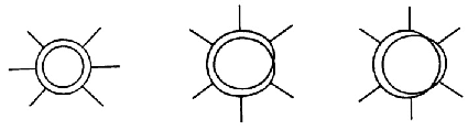
(a) (b) (c)
In 1984, M. Green and J. H. Schwarz realized the cancellation of anomalies in type I superstring theory with the gauge group . Now we consider only the effective field theory point of view. For further details and the string formalism, we remand to the original papers [23]. In ten-dimensional theories gauge anomalies, mixed anomalies, and gravitational anomalies were expected to arise from a hexagon loop diagram ( then ). The anomaly cancels because of an extra contribution from a 2-form field, , which is one of the new states predicted by string theory (if we can think of a gauge vector as column, we can think of as a matrix). For the special choice of the gauge group or , however, the anomaly factorizes and may be cancelled by a tree diagram. The tree diagram describes the exchange of a virtual . It is somewhat counterintuitive to see that a tree diagram cancels a one-loop diagram, but in reality, both of these diagrams arise as one-loop diagrams in superstring theory, in which the anomaly cancellation is more transparent. In Fig. 3.3 and Fig. 3.4 are depicted respectively the diagrams involved in the string theory mechanism and in the effective field theory mechanism. The diagram (a) and (b) of Fig. 3.3 are generated by planar open string loops and we can naively say that they produce the effective fermionic hexagon diagram, while the diagram (c) is a non planar open string loop. However the latter can also be viewed as the tree level propagation of a closed string. One of the closed string states is the field, so we can naively say that this diagram, apart from contributing to the diagram of Fig. 3.4(a), produces the effective tree level diagram of Fig. 3.4(b).
††feynman-diagram: (Feynman diagram, (x1) ††feynman-diagram: (Feynman diagram, (x1)
(a) (b)
Let us see how the mechanism works for the gauge group. The low energy effective field theory is supergravity coupled to supersymmetric Yang-Mills theory. The bosonic action is given by
| (3.42) | |||||
where and are respectively the Yang-Mills and the gravitational coupling, is the determinant of the zehnbein and is a scalar field. The Yang-Mills field strength is defined (in the language of forms) by
| (3.43) |
where . The field strength associated with the two-form potential of the supergravity multiplet is defined by
| (3.44) |
where is the Yang-Mills Chern-Simons three-form
| (3.45) |
and is the Lorentz group Chern-Simons three-form
| (3.46) |
Here is the local Lorentz connection and is the Lorentz curvature two-form. The Chern-Simons forms (3.45) and (3.46) satisfy
| (3.47) | |||
| (3.48) |
Under infinitesimal local Yang-Mills transformation (with parameter ) and local Lorentz transformation (with parameter ), the fields transform as follows
| (3.49) | |||
| (3.50) | |||
| (3.51) |
Consider the Yang-Mills hexagon anomaly. The analysis of [24] relates the anomalies to a formal expression in 12 dimensions, namely the gauge invariant two-form , where
| (3.52) |
The last equality is true only for the gauge group. This can be expressed as
| (3.53) |
where is defined by
| (3.54) |
Similarly, applying an infinitesimal gauge transformation, one defines by
| (3.55) |
In the case of Yang-Mills hexagon, the consistent anomaly is
| (3.56) |
where the anomaly factor can be deduced from [24]. This anomaly can be cancelled by adding to the effective action
| (3.57) |
The non trivial transformation of in eq. (3.51) is the key of the cancellation
| (3.58) |
The diagram (b) in Fig. 3.4 is built by connecting the vertex in eq. (3.57) to the vertex (contained in the term) in eq. (3.42) by a propagator.
This is the cancellation of the Yang-Mills anomaly for the gauge group . The cancellation of the gravitational and mixed anomaly goes in a similar way and we remand to the original paper [23] for details.
In the following section we will see that something similar happens in four-dimensional theories. The anomaly, as shown in the previous section, is related to a triangle loop diagram and it can be cancelled by the contribution of an extra field, the axion22 2 In four dimensions the axion is dual to a 2-form. See for instance [25] for the GS-mechanism with this duality manifest..
3.3.2 Triangular Anomaly
Let us go back to the Lagrangian (3.1). Let be anomaly free i.e. eq. (3.36) holds, but let be anomalous i.e. . We use the GS mechanism to restore gauge invariance. As stated before, we need to modify the Lagrangian inserting a new field, the axion . So we get
| (3.59) |
contains the couplings of
| (3.60) | |||||
The first row is the Stückelberg Lagrangian [26]. The axion is uncharged under and and it transforms as
| (3.61) |
so that the Stückelberg Lagrangian is gauge invariant. The reason to have these terms is to give a mass to the gauge vector without using a proper scalar potential breaking some symmetries . The axion is the third degree of freedom of the massive , so it is an unphysical particle, a Goldstone boson. The second row of terms contains the GS couplings33 3 We use the notation . () which are not gauge invariant because of the transformation. These terms are directly involved in the anomaly cancellation procedure and their form is dictated by the form of the WIs for the triangle amplitudes.
contains the so called Generalized Chern-Simons couplings
| (3.62) |
which are antisymmetric trilinear interactions of gauge vectors. Also these terms are not gauge invariant and they will play some role in the GS mechanism.
The cancellation of the anomalies will fix the GS and GCS couplings. In the following we will show two different approaches to the GS mechanism: using WIs or using the effective Lagrangian. Obviously we will get the same result.
3.3.3 Ward Identities for massive gauge fields
As stated before, the WIs on a Feynman amplitude reflect the gauge invariance of a quantum field theory. They can be written in the diagrammatic form showed in Fig. 3.2. However, it is well known that gauge invariance can be achieved only with massless vector fields. On the other side we experience the existence of not only physical massless vectors, with two degrees of freedom, such as the photon, but also of physical massive vectors, with three degrees of freedom, such as the . The Proca Lagrangian describes the last one, but it is not gauge invariant since an explicit mass term for the vector breaks the gauge invariance. Fortunately, it is well known that we can avoid such a problem with the Higgs or with the Stückelberg mechanism. We add in a proper way (which depends on the mechanism used) a scalar field (Goldstone boson) and vector mass terms to the massless vector Lagrangian. This scalar field will become the third degree of freedom of the massive vector. However this will become manifest after a unitary gauge fixing. In this gauge the Goldstone bosons are set equal to zero, we turn back to the Proca Langrangian and the physical degrees of freedom are manifest. In this way we can achieve a gauge theory with a massive vector and since we have the gauge invariance we expect that the WIs hold. But now we have to take into account that we have a new degree of freedom coming from the Goldstone boson, which is directly related to the gauge sector. This modifies the WIs, which get the diagrammatic form showed in Fig. 3.5 [27].
††feynman-diagram: (Feynman diagram, (x4) ( ††feynman-diagram: (Feynman diagram, (x4)
As we can see, now we have a contribution coming from the Goldstone boson44 4 For a brief demonstration see Appendix D.2.. To clarify the point we consider a specific example: the decay in the SM.
( ††feynman-diagram: (Feynman diagram, (x3) ) + ( ††feynman-diagram: (Feynman diagram, (x3) ) = 0
The Feynman amplitude of the process is given by (for the Feynman rules see Appendices C.2 and C.3)
| (3.63) |
where , and . The WI for the process is given in Fig. 3.6. The first term is
| (3.64) | |||||
where is the electron mass and we used the equation of motion of the spinors
| (3.65) | |||||
| (3.66) |
The second term is
| (3.67) | |||||
where we used and eq. (2.84). Summing the eq. (3.64) and (3.67) we get
| (3.68) |
in agreement with the result showed in Fig. 3.5.
3.3.4 Ward Identities and Anomaly Cancellation
Let us go back to the anomaly cancellation procedure. We focus on the anomaly. The WIs (3.29), (3.30) and (3.31) modified because of the presence of GS and GCS couplings. Using Fig. 3.5, we get the WIs for the amplitude expressed in diagrammatic form in Fig. 3.7.
††feynman-diagram: (Feynman diagram, (x6) + ††feynman-diagram: (Feynman diagram, (x3) ††feynman-diagram: (Feynman diagram, (x3)
††feynman-diagram: (Feynman diagram, (x6) + ††feynman-diagram: (Feynman diagram, (x3)
††feynman-diagram: (Feynman diagram, (x6) + ††feynman-diagram: (Feynman diagram, (x3)
The Feynman rules for the GS mechanism are given in Appendix C.1. We denote by the contribution coming from the GS coupling in Lagrangian (3.60)
| (3.69) |
and we denote by the contribution from the GCS coupling in Lagrangian (3.62)
| (3.70) |
The WIs in Fig. 3.7 correspond to
| (3.71) |
Using eq. (3.29), (3.30) and (3.31), the last two identities imply
| (3.72) |
and the first identity becomes
| (3.73) |
In the same way55 5 The momenta of the triangle are so that on the incoming line we have the vector., the cancellation of the remaining anomalies gives
| (3.74) | |||
| (3.75) |
where we used different shift parameters and respectively for the new triangles and . However as stated in the end of Section 3.1 and done in eq. (3.74), must be fixed to because we have three equal external vectors. It is worth noting that the GCS coefficients are determined in terms of the ’s by the WIs, while the ’s depend only on the free parameter , which is related to the mass of the anomalous . Moreover the GCS couplings depends on the scheme of the anomaly distribution so they do not contain any physical information (see Section 3.5). We can always cancel them with a particular choice of the shift parameters, in fact they are also called GCS counterterms because they parametrize the arbitrariness of the scheme of the anomaly distribution in the anomaly cancellation procedure. On the contrary, the GS coupling does not depend to any shift parameters and so they have some physical relevance as we will show in the computation of the amplitudes in Section 3.5.
3.3.5 Effective Lagrangian
Now we show the anomaly cancellation using the variation of the effective Lagrangian. As before we focus on the amplitude. The WIs (3.29), (3.30) and (3.31) induce the following variations on the 1 loop effective Lagrangian. For
| (3.76) | |||||
| (3.77) |
we have
| (3.78) | |||||
| (3.79) |
The requirement of gauge invariance implies
| (3.80) | |||||
| (3.81) |
The gauge variations for the axion Lagrangian are
| (3.82) | |||||
| (3.83) |
and for the GCS terms are
| (3.84) | |||||
| (3.85) | |||||
where we used . Then eq. (3.81) implies
| (3.86) |
Substituting this result into eq. (3.80), we get
| (3.87) |
We showed the anomaly cancellation procedure in two different ways, the WI method or the effective Lagrangian one. Dependently on what we need to compute we will choose the most convenient procedure.
3.4 Supersymmetric Green-Schwarz mechanism
In this section we illustrate how to supersymmetrize what we did in the previous section. The supersymmetric version of eq. (3.60) and (3.62) are (see [25] and [28])
| (3.88) | |||||
| (3.89) | |||||
where the ’s and the ’s are the gauge superfields and the corresponding superfield strength, and S is the Stückelberg multiplet
| (3.90) |
which transforms under the as
| (3.91) |
The component fields of are the complex scalar , where is the saxion and is the axion, and the spinorial field which is called axino. To fix the ’s and ’s parameter we act on the bosonic part as we did in Section 3.3, since the supersymmetric part will be fixed by supersymmetry, or we act directly on the superfields. We show the last method for the case. Under the gauge transformations
| (3.92) |
we have
| (3.93) | |||||
| (3.94) |
| (3.95) | |||||
| (3.96) |
| (3.97) | |||||
| (3.98) |
The requirement of gauge invariance will impose the following conditions
| (3.99) | |||
| (3.100) | |||
whose solutions are the eq. (3.72) and (3.73). Analogously for the other anomalies.
3.5 Computation of the amplitudes
In this section we show how we compute the 1 loop amplitudes66 6 For a massive fermionic triangle see Appendix D.3. involving three external vectors. As usual we focus on the case since the generalization to the other cases is straightforward.
Before going on we recall the Rosenberg parametrization77 7 For a demonstration of the Rosenberg parametrization see Appendix D.3. [29]. The amplitudes (3.7), (3.8), (3.9) and (3.10) can be written as
| (3.101) |
with and where
| (3.102) |
In terms of the Rosenberg parametrization the dependence of (3.17) is contained only in and (which are superficially divergent). However, using the WIs (3.26), (3.27) and (3.28) it is possible to show that they can be expressed in terms of as
| (3.103) |
Analogously for the VAV, VVA and AAA triangles.
We can act in the same way for the amplitude. The total fermionic triangle can be written as
| (3.104) |
where is the parametrization (3.101). Imposing the eq. (3.29), (3.30) and (3.31) we find that
| (3.105) |
and the amplitude, as we know, is not uniquely defined. The anomaly cancellation will solve this problem. In the standard case we have so the amplitude is uniquely defined but identically zero. Instead with the GS mechanism, the final amplitude will not be zero. In this case we have
| (3.106) |
The GCS terms can be reabsorbed by the following redefinitions
| (3.107) |
where
| (3.108) | |||||
with
| (3.109) |
Using eq. (3.72) and (3.105) we get
| (3.110) |
that relate and to the other ’s. So we have removed the dependence of the fermionic triangle, thanks to the GCS coupling, and the amplitude is uniquely defined and it obeys the following WIs
| (3.111) |
Finally the theory is gauge invariant, but in this case the amplitude is different from zero. This result does not depend on the scheme of the anomaly distribution.
Chapter 4 MiAUMSSM. Model building
One of the most attractive scenario for physics beyond the SM is the existence of additional massive neutral gauge bosons (for a recent review see [30] and references therein; for some recent works we suggest [31]-[37]). They could be one of the first discoveries at LHC if their mass is in the range of a few TeV. Many different models have been developed in the past in order to investigate this possibility. The mass could be acquired in a variety of ways: from Kaluza-Klein modes to a standard Higgs mechanism or even the Stückelberg mechanism [26]. The latter is common to low energy effective field theories which appear anomalous. The anomaly cancellation is achieved by the GS mechanism which ensure the consistency of these models [23, 38].
In string theory anomalous ’s are very common. D-brane models contain several abelian factors, living on each stack of branes, and they are typically anomalous [38]-[46]. In the presence of these anomalous ’s, the Stückelberg mixing with the axions cancels mixed anomalies, and renders the “anomalous” gauge fields massive. The masses depend non-trivially on the internal volumes and on other moduli, allowing the physical masses of the anomalous gauge bosons to be much smaller than the string scale (even at a few TeV range) [43]. For further works on these topics see [47]-[63].
This chapter is entirely based on [1], where we presented for the first time our model: the Minimal Anomalous Extension of the MSSM (MiAUMSSM).
4.1 Preliminaries
We study an extension of the MSSM11 1 Since we do not discuss phenomenological consequences, the treatment of all this section is before the insertion of the coupling constant using . by the addition of an abelian vector multiplet . We assume that all the MSSM fields are charged under the additional vector multiplet , with charges that are given in Table 4.1, where are the left handed quarks and leptons respectively while are the right handed up and down quarks and the electrically charged leptons. The superscript stands for charge conjugation. The index denotes the three different families. are the two Higgs scalars.
| SU(3)c | SU(2)L | U(1)Y | U(1) | |
|---|---|---|---|---|
In order to gain in flexibility, our model is only string inspired: we do not commit to a specific brane model and this is why the charges are not fixed, even if the effective cut-off is related to the mass of the . Since our model is an extension of the MSSM, the gauge invariance of the superpotential (2.2), that contains the Yukawa couplings and a -term, put constraints on the above charges
| (4.1) |
Thus, , and are free parameters of the model.
The extra vector multiplet generically is anomalous and consistency of the model requires an additional Stückelberg multiplet with the proper couplings as well as GCS terms. For the complete Langrangian of the model see Appendix B.2.
4.1.1 Anomalies and GS mechanism
As showed in Section 3.2, the MSSM is anomaly free. All the anomalies that involve only the , and factors vanish identically. However, triangles with in the external legs in general are potentially anomalous. These anomalies are22 2 We are working in an effective field theory framework and we ignore throughout the Thesis all the gravitational effects. In particular, we do not consider the gravitational anomalies which, however, could be cancelled by the GS mechanism.
| (4.2) | |||||
| (4.3) | |||||
| (4.4) | |||||
| (4.5) | |||||
| (4.6) |
where runs over the fermions in Table 4.1, is the corresponding charge, is the hypercharge and , are the generators of the and algebras respectively. In our notation . All the remaining anomalies that involve s vanish identically due to group theoretical arguments (see Chapter 22 of [20]). Using the charge constraints (4.1) we get
| (4.7) | |||||
| (4.8) | |||||
| (4.9) | |||||
| (4.10) | |||||
| (4.11) |
Notice that the mixed anomaly between the anomalous and the nonabelian factors vanishes identically.
Many models have been developed in the past where all the anomalies (4.7-4.11) vanish by constraining the charges (see [30] and references therein). On the contrary, in this Thesis we assume that the is anomalous, i.e. (4.7)-(4.11) do not vanish. Consistency of the model is achieved by the GS mechanism showed in Sections 3.3 and 3.4. The axionic Lagrangian now reads
| (4.12) | |||||
where the index runs over the and gauge groups respectively. The Stückelberg multiplet is given in (3.90) and transforms under the as
| (4.13) |
where is a constant. The lowest component of is a complex scalar field . We assume that the real part gets an expectation value by an effective potential of stringy or different origin and contributes to the coupling constants as
| (4.14) |
where is the redefined coupling constant and the gauge factors take the values . The first line in (4.12) is the Stückelberg Lagrangian [26] of the which is gauge invariant and provides the kinetic terms and the axion- mixing. The second line is not gauge invariant and provides the GS couplings that participate in the anomaly cancellation procedure. Notice that in (4.12) the sum over omits the case since there is no mixed anomaly between the and the factors as from eq.(4.10), i.e. . The values of the other constants, , are fixed by the anomalies.
At first sight our Lagrangian (see Appendix B.2) may not look like the most general possible one. In particular, an explicit Fayet-Iliopoulos term could be added. It is well known that in certain string models (see, e.g. [64, 65]), an one-loop FI term is absent, even if . This is in apparent conflict with the observation [66] that in field theory a quadratically divergent FI term is always generated at one loop. The solution to this paradox is that in the low-energy Lagrangian there should be a counterterm, which compensates precisely, i.e. both the divergent and the finite part of, the one-loop contribution. We do not write explicitly this counterterm, since its exact expression is model and regularization dependent, but we implicitly assume that such a cancellation occurs. As mentioned before, also the terms responsible for the cancellation of gravitational anomalies are omitted.
Expanding in component fields, using the Wess-Zumino gauge and substituting by its VEV we get
| (4.15) | |||||
where we omit terms which are coming from , since they are absorbed in the coupling constant redefinition (4.14). As stressed in the previous chapter, this mechanism cancels some mixed anomalies and in addition provides a mass term to the anomalous . Therefore, the anomalous behaves like the usual extensively studied in the past.
For what concern the GCS terms we have
| (4.16) | |||||
and their expression in component fields
| (4.17) | |||||
The constants , and are fixed by the cancellation of the mixed anomalies.
The cancellation of anomalies goes in the same way as in Sections 3.3 and 3.4 so we give only the results
| (4.18) |
For simplicity we chose a symmetric distribution for all the anomalies (see the discussion at the end of Section 3.1). For the anomaly cancellation in the broken phase we remand to a specific case in Section 5.2.1 and to our paper [1].
Before going on we want to spend other few words on these anomalies. In our model there are two extra states in the neutral fermionic sector, namely the axino and the primeino (see Section 4.2.7) which do not contribute to the fermionic loop. The remaining MSSM fermionic states are a bino, a wino and the two higgsinos. Both and gauginos do not contribute to the fermionic loop due to group theoretical arguments (see Section 28.1 of [67]). The higgsino eigenstates do not participate because the contribution is cancelled by the one. This is due to the fact that each diagram is proportional to an odd product of charges and the two higgsinos have opposite charges (see Table 4.1 and the constraints (4.1)). Therefore only SM fermions give the relevant contribution to the anomalies (4.7)-(4.11).
4.1.2 Soft breaking terms
Since we added new matter content to the MSSM Lagrangian we expect that new soft breaking terms can be added to the theory. The total soft breaking Lagrangian can be written as
| (4.19) |
where is the MSSM soft breaking Lagrangian given in eq. (2.10) and
| (4.20) |
where is the gaugino of the added and is the axino. We allow a soft mass term for the axino since it couples only through GS interactions and not through Yukawa interactions [68]. Notice also that a mass term for the axion is not allowed since it transforms non trivially under the anomalous gauge transformation (4.13).
4.2 Model setup
In this section we analyze the effects of the additional terms on the rest of the Lagrangian. From now on we work with the Lagrangian (B.8) after substitution .
4.2.1 Kinetic diagonalization of U(1)’s
As we mentioned before, the Stückelberg multiplet contains a complex scalar field whose real part gets an expectation value that modifies the coupling constant (4.14). Therefore, the second line in (4.12) contributes to the kinetic terms for the gauge fields and the term gives a kinetic mixing between the and gauge bosons. We have
| (4.21) |
with . In order to diagonalize the kinetic terms, we use the matrix
| (4.22) |
where and . Let us stress that in this case the mixing is a consequence of the anomaly cancellation procedure. Note that, since (see eq. (4.18)), where is the mass of the anomalous that we assume to be in the TeV range, this mixing is tiny and can be ignored for our purposes.
4.2.2 and terms
The additional fields give rise also to and terms. More precisely, term contributions come from: (i) the kinetic terms of chiral multiplets and (ii) the axionic Lagrangian (4.12), providing
where denotes, as usual, the gauge group factors, are the lowest components of the -th chiral multiplet (except the multiplet which contains the axion) and , , are the generators of the corresponding gauge groups, . Solving the equations of motion for the D’s and substituting back we obtain
| (4.24) |
| (4.25) | |||||
| (4.26) | |||||
| (4.27) |
Similarly, the term contributions are
| (4.28) | |||
where the first line is the standard MSSM term contribution while the second line contains the new Stückelberg terms. Solving the equation of motion
| (4.29) | |||||
Eq. (4.29) can also be written in the basis (4.22), but we will not need this term in the following.
We would like to mention that no and terms are coming from the GCS since they include only vector multiplets in an antisymmetric form. Our results are in accordance with [63].
4.2.3 Scalar potential
As we have seen in the previous section, the additional terms (4.29) do not give any contribution to the scalar potential. The , and terms (see eq. (4.25), (4.26) and (4.27)) provide the usual contributions to the MSSM potential. The only new contribution comes from the first line of (4.24). Thus the scalar potential can be written as
| (4.30) | |||||
| (4.31) |
Solving the equations for the minima of the potential
| (4.32) |
we get for all the sfermions as in the MSSM case. Inserting back these VEVs into (4.30) we get the following Higgs scalar potential
| (4.33) | |||||
which can be brought to the same form of the MSSM potential (see eq. (2.40)), after the following redefinitions
| (4.34) |
where
| (4.35) |
At the minimum, we recover the MSSM result for the Higgs charged components. Defining as usual , and we can still write the tree level conditions for the electroweak symmetry breaking as
| (4.36) | |||||
| (4.37) |
in complete analogy with the MSSM case (using ’s).
4.2.4 Higgs sector
It is worth noting that in our model there is no axi-Higgs mixing. This is due to the fact that we do not consider scalar potential terms for the axion (on the contrary to [44]).
After the electroweak symmetry breaking we have four gauge generators that are broken, so we have four longitudinal degrees of freedom. One of them is the axion, while the other three are the usual NG bosons coming from the Higgs sector.
As it was mentioned above, the potential has the standard MSSM form, upon the redefinitions (4.34). Since the discussion goes in the same way as Section 2.4.2, here we give only the main ideas. Higgs scalar fields consist of eight real scalar degrees of freedom: three of them are the NG bosons , . The remaining five Higgs scalar mass eigenstates consist of two CP-even neutral scalars and , one CP-odd neutral scalar and a charge scalar as well as its charge conjugate with charge . The gauge-eigenstate fields can be expressed in terms of the mass eigenstate fields as
where the orthogonal rotation matrices are the same as in (2.65). Acting with these matrices on the gauge eigenstate fields we obtain the diagonal mass terms. Replacing the tilde parameters (4.34) we obtain the masses (compare with eq. (2.67), (2.68) and (2.69))
| (4.52) | |||||
| (4.53) | |||||
| (4.54) |
and the mixing angles (compare with eq. (2.71))
| (4.55) |
Notice that only the and masses modified with respect to the MSSM, due to the additional anomalous .
4.2.5 Neutral Vectors
There are two mass-sources for the gauge bosons: (i) the Stückelberg mechanism and (ii) the Higgs mechanism. In this extension of the MSSM, the mass terms for the gauge fields are given by
| (4.56) |
are the spin 1 components of the vector multiplets . The gauge boson mass matrix is
| (4.57) |
where and the lower dots denote the obvious terms under symmetrization. After diagonalization, we obtain the eigenstates
| (4.58) | |||||
| (4.59) | |||||
| (4.60) |
and the corresponding masses
| (4.61) | |||||
| (4.62) | |||||
where is the mass parameter for the anomalous and it is assumed to be in the TeV range. Due to their complicated form, the eigenstates and eigenvalues of (4.57) are expressed as power expansions in and keeping only the leading terms. Higher terms are denoted by .
The first eigenstate (4.58) corresponds to the photon and it is exact to all orders. It slightly differs from the usual MSSM expression (2.82) due to the kinetic mixing between and .
For the rest of the Thesis, we neglect the kinetic mixing contribution since they are higher loop effects which go beyond the scope of the Thesis. Then the rotation matrix from the hypercharge to the photon basis, up to is
where .
4.2.6 Sfermions
In general, the contributions to the sfermion masses are coming from (i) the and terms in the superpotential and (ii) the soft-terms. However, in our case, the new contribution comes only from the terms
| (4.78) | |||||
where the stand for all possible sfermions.
4.2.7 Neutralinos
With respect to the MSSM, now we have two new fields: and . Thus, we have
| (4.79) |
where
| (4.80) |
The neutralino mass matrix gets contributions from (i) the MSSM terms, (ii) the couplings, (iii) the new soft-breaking terms , (iv) the Stückelberg action and (v) the terms. Finally, we obtain the symmetric matrix
| (4.81) |
where , , and are the masses coming from the soft breaking terms (4.19), and
| (4.82) | |||||
with . It is worth noting that the terms and kinetic mixing terms are only higher order corrections and they can be neglected in the computations of the eigenvalues and eigenstates.
Chapter 5 MiAUMSSM. Phenomenology
In this chapter we discuss some phenomenology consequences of the model showed in Chapter 4. We focus on the simple but still interesting case . In this case there is no mixing between the and the other SM gauge fields therefore (see (4.2.5)). Then the couples only to SM fermions and their corresponding superpartners. There is no tree level interaction between the and the ’s or the neutralinos or the charginos since the corresponding couplings are proportional to . Moreover, as we will see in the following, this simple choice implies interesting properties of the involved in fermionic triangles.
First of all we will study the tree level decays of the into fermions and the anomalous decays into neutral gauge bosons. We will check the anomaly cancellation in the broken phase and we will also give some prediction about these processes in LHC.
Then we will pass to the supersymmetric sector. We will consider the case in which the axino is the LSP and we will check if the prediction for the relic density is in agreement or not with the current experimental bounds.
5.1 Tree level decays
First of all we discuss the tree level decays of the . As suggested in the introduction, the tree level final states can only be fermions or sfermions. Since this is a standard part we do not spend much time in details. We remember that we are in the case .
5.1.1 Fermions
The Lagrangian describing the interaction of the with SM fermions is given by
| (5.1) |
where , is the usual Dirac spinor (see eq. (3.3)) and the vectorial and axial couplings are defined as
| (5.2) |
and listed in Table 5.1.
| , , | ||
| , , | ||
| , , | ||
| , , |
The decay rate is given by
| (5.3) |
where the colour factor for leptons (quarks) and the kinematic factors
| (5.4) |
take into account the fermion mass .
5.1.2 Sfermions
The Lagrangian describing the interaction of the with sfermions is given by
| (5.5) |
where the is for left (right) handed sfermions respectively and with and given in eq. (5.2). The decay rate for decay to sfermions is calculated to be
| (5.6) |
where the colour factor is defined as in the fermion case and is the sfermion mass.
In the case of non-negligible sfermion mixing (such as the top squark) we must work in the mass eigenstate basis. The decay width is similar to (5.6) with the appropriate couplings, except that the phase space factor in the case of different mass decay products is . For details see for instance [32].
5.1.3 Numerical results
The tree level decay width for a , is given by the sum of the decay rates given in the previous sections
| (5.7) |
We focus on the case TeV. The reason will be clear in Section 5.3. Since we suppose that the LSP has a mass higher than 500 GeV (see Section 5.4.2 for scenarios in which this happens), the sfermion masses are heavier that , so they cannot be produced by an on-shell decay. We have
| (5.8) | |||||
where we used eq. (5.3). Since the will be detected at LHC through is decays into electric charged leptons we give also the branching ratio (BR) for the decay into an electron-positron pair
| (5.9) | |||||
The results are plotted in Fig. 5.1 in the form of contour plots in the plane . Our choices for , , and are in agreement with the current experimental bounds [69].


(a) (b)
The tree level decay width has elliptic contours since eq. (5.8) is the equation of an ellipse in the plane . Concerning the let us observe that if the quarks and the leptons have the same mass and the same couplings, then the branching ratio will be simply the inverse of the total number of fermions which is the number of leptons (6) plus the number of quarks (6) times the color factor (3)
| (5.10) |
This is the reason why has a lot of values less then 5%. In a region of parameters the most important quantity is the number of the possible final states.
5.2 Anomalous Decays
In this section we compute the amplitudes for the on-shell decays of the into neutral gauge bosons. The SM fermion interaction terms with SM neutral gauge bosons are
| (5.11) |
where denote the electric charges, and are the vectorial and axial couplings with and and are the vectorial and axial couplings with , respectively. They are listed in Table 5.2.
| , , | |||||
| , , | |||||
| , , | |||||
| , , |
We remind that, for , the is decoupled for the SM neutral gauge sector, so and the SM coupling constants are given in eq. (2.87) and (2.88). For the corresponding Feynman rules see Appendices C.2 and C.4.
A priori we could have three possibilities: , and . But the on-shell decay is prohibited by the Landau-Yang theorem [70], for which we give a brief demonstration in Appendix D.4. This decay is permitted only if at least one of the two photons is off-shell. Moreover with the choice , we have that the electric charged fermions have only vectorial couplings with the (see Table 5.2), so the fermionic triangle loop for the decay has three vectorial vertices, so the corresponding amplitude is zero because of the Furry theorem [71]. So in our case, the only possible decays in the neutral gauge sector (on and off-shell) are and . However we remind that we are interested only in on-shell decays.
Since there is no tree level interaction between the and neutralinos or charginos, no contribution to the fermionic triangles is given by the SUSY sector so, we get the same results, for what the decays of interest are concerned, of non-SUSY models.
5.2.1 Anomaly cancellation
Before going on in our computations we check that the anomaly cancellation still holds in the broken phase. We focus on the process since the extension to the other cases is straightforward. In the broken phase, additional contributions coming from the NG boson () exchange must be added. The corresponding WI’s, given in diagrammatic form in Fig. 5.2, are
| (5.12) | |||||
| (5.13) | |||||
| (5.14) |
where is the fermionic loop with external , and , is the GCS coupling for the vectors cited above, is the GS coupling between the axion, the and the photon and is the fermionic loop with external , and .
††feynman-diagram: (Feynman diagram, (x6) + ††feynman-diagram: (Feynman diagram, (x3) ††feynman-diagram: (Feynman diagram, (x3)
††feynman-diagram: (Feynman diagram, (x6) + ††feynman-diagram: (Feynman diagram, (x3) ††feynman-diagram: (Feynman diagram, (x6)
††feynman-diagram: (Feynman diagram, (x6) + ††feynman-diagram: (Feynman diagram, (x3)
The fermionic triangle is given by
| (5.15) |
where is given by (D.19) and
| (5.16) |
So we have (compare with eq. (D.40))
| (5.17) | |||||
| (5.18) | |||||
| (5.19) |
since we choose a symmetric distribution of the anomaly. The integral is given in eq. (D.42) and is defined after (3.101). Using eq. (2.87) and (2.88) and computing we get
| (5.20) | |||||
| (5.21) | |||||
| (5.22) |
The corresponding GCS coupling is given by the proper combination of the GCS couplings in the hypercharge basis (see Fig. 5.3a)
††feynman-diagram: (Feynman diagram, (x3) ††feynman-diagram: (Feynman diagram, (x3) ††feynman-diagram: (Feynman diagram, (x3) (a)
††feynman-diagram: (Feynman diagram, (x3) ††feynman-diagram: (Feynman diagram, (x3) ††feynman-diagram: (Feynman diagram, (x3) (b)
| (5.23) |
where the rotation factors are
| (5.24) |
So we get
| (5.25) | |||||
where we used eq. (4.18), (4.8) and (4.9). Then using eq. (5.22) we have
| (5.26) | |||||
and eq. (5.14) is verified. From eq. (5.20) and (5.25) we easily obtain
| (5.27) |
The corresponding GS coupling is given by the proper combination of the GS couplings in the gauge interaction basis (see Fig. 5.3b)
| (5.28) | |||||
where we used eq. (4.18), (4.8), (4.9) and (5.24). We remember that since , (see eq. ()). Then using eq. (5.27) we have
| (5.29) |
and eq. (5.12) is verified. From eq. (5.21) and (5.25) we easily obtain
| (5.30) |
Computing the Feynman amplitude for diagram we find
| (5.31) | |||||
where we used , , eq. (2.88) and (4.62) for , the values for given in Table 5.2 and the definition of given in eq. (5.16). Then summing eq. (5.30) and (5.31) we get
| (5.32) |
and also eq. (5.13) is verified. So we checked the consistence of the anomaly cancellation in the broken phase.
5.2.2
We calculate the decay rate for . We compute all the relevant diagrams in the gauge, thus removing the interaction vertex that involves the massive gauge bosons and the Stückelberg or NG boson. Therefore, the only diagrams that remain are the fermionic loop, the GCS vertex and a not anomalous remnant contribution (Fig. 5.4). It is possible to show that the last blob-diagram, that involves several diagrams, is equal to zero. For the interested reader we give further details in Appendix D.5.
††feynman-diagram: (Feynman diagram, (x3) =
††feynman-diagram: (Feynman diagram, (x6) + ††feynman-diagram: (Feynman diagram, (x3) + ††feynman-diagram: (Feynman diagram, (x3)
The decay rate for the process is given by
| (5.33) |
where is the total scalar amplitude and is the momentum of the outgoing vectors in the CM frame
| (5.34) |
The square of the total scalar amplitude is given by
| (5.35) |
where are the polarizations of the gauge bosons, and is the Feynman amplitude of the process. The factor comes from the average over the helicity states. The polarizations obey to the following completeness relations
| (5.36) | |||||
| (5.37) | |||||
| (5.38) |
where (5.38) gives only the relevant part of the sum over helicities. Other terms are omitted since they give vanishing contributions to the decay. The amplitude is given by the sum of the fermionic triangle plus the proper GCS vertex
| (5.39) |
where and are given in eq. (5.15) and (5.25). It is convenient to express the triangle amplitude by using the Rosenberg parametrization [29] (see also Appendix D.3)
| (5.40) | |||||
where
| (5.41) |
and are finite integrals (their explicit forms are given in (D.25)), is defined after (D.24) and is given in eq. (5.16). and are naively divergent by power counting and so they must be regularized. We compute them by using the Ward identities. In this way it is possible to express and in terms of the finite integrals and . The GCS term has the following tensorial structure
| (5.42) |
so it can be absorbed by shifting the first two coefficients of the Rosenberg parametrization for the triangle (see Section 3.5). The resulting amplitude can be written as
| (5.43) | |||||
The WIs (5.12), (5.13) and (5.14) now read
| (5.44) | |||||
| (5.45) | |||||
| (5.46) |
where and are the and masses respectively. Using the results of the previous section we obtain
| (5.47) | |||||
| (5.48) | |||||
| (5.49) |
and inserting (5.43) into the above identities we get
| (5.50) |
with
| (5.51) |
where is the integral given in (D.42). Substituting from (5.50) into the amplitude (5.43) and performing all the contractions we finally obtain
| (5.52) | |||||
5.2.3
The computations are similar to the previous case so we point out only the differences with the other decay. Mutatis mutandis, the decay rate for the process is given in (5.33) with the proper amplitude and
| (5.53) |
The square of the total scalar amplitude is given by
| (5.54) |
where the amplitude is always the sum of the fermionic triangle and the GCS term. The contribution to the fermionic triangle is
| (5.55) | |||||
where runs over all the neutrinos while the ’s are given by (D.18), (D.19), (D.20), (D.21). Using the fact that for the three neutrino families we have and we write the total amplitude (the sum of the triangles plus GCS terms) as
| (5.56) | |||||
with
| (5.57) |
where
| (5.58) |
with for neutrinos and for the other fermions. The WIs now read
| (5.59) | |||||
| (5.60) | |||||
| (5.61) |
leading to
| (5.62) | |||||
| (5.63) | |||||
| (5.64) |
From these equations we find the following values for and
| (5.65) | |||||
| (5.66) |
with
| (5.67) |
where is the integral given in (D.42). Substituting back into the amplitude and performing all the contractions we finally obtain
| (5.68) |
5.2.4 Numerical Results


We show some numerical computations for the two decay rates and . They depend on the free parameters of the model, i.e. the couplings , and the mass of the , since . We show our results in Fig. 5.5-5.7 in the form of contour plots in the plane for and TeV. Our choices for , , and are in agreement with the current experimental bounds [69].
The darker shaded regions correspond to larger decay rates. The white region corresponds to the value GeV that can be considered as a rough lower limit for the detection of the corresponding process. It is worth noting that increasing the mean value of the decay rate of grows while the one of decreases. We would also like to mention that increasing the iso-decay rate contours in the plot rotate clockwise getting more and more parallel to the -axis. This effect is due to the fact that the contribution of the triangle diagram with the top quark circulating inside the loop becomes the dominant contribution for high . In this case the decays strongly depend on the top quark coupling while the lepton couplings become irrelevant. Finally, we find that the region that gives the largest values (of order of GeV) of the decay is for TeV and for , .
5.3 LHC prediction


To estimate the number of the decays that can be observed at LHC we shall use the narrow width approximation,
| (5.69) |
where is the total number of produced and is the branching ratio of the decay of interest. We remind that we can use such approximation if . For our choice of parameters, the maximum value will be for and TeV, so and the latter inequality holds.
The total number of is where the luminosity and 1 year. Finally is the production cross section [30]
| (5.70) |
where are the quark (or antiquark ) structure functions in the proton, and the momentum fractions are
| (5.71) |
The formula (5.70) does not take into account the gluon contribution inside the proton. The gluons can only contribute with the fermionic loop triangle. There is no GCS contribution since there is no anomaly (see eq. (4.10)). However the vertex is vectorial like, as the corresponding vertex with the for (see Table 5.1), so we have a triangle which is zero because of the Furry theorem [71]. Then, in this case, we do not have any gluon contribution.
We integrate numerically the PDFs using a Mathematica package [72]. In Fig. 5.8 we show the result for at TeV. We can see that the number of the produced falls off exponentially with , so we shall focus on the case TeV. As said before, we assume that the LSP has a mass higher than 500 GeV (see Section 5.4.2), so that we can ignore sparticles contribution in the computation of the branching ratios.
In Fig. 5.9, we estimate the number of decays for 1 year of integrated luminosity. We can see that in a wide region of parameter the number of events is larger then ten thousand. This gives a lot of chance to discover a in LHC.
In the case TeV the most favorite anomalous decay is . In Fig. 5.10, we estimate the number of decays for 1 year of integrated luminosity which turns out to be for large values of the couplings and .
5.4 Axino Dark Matter
Assuming the conservation of R-parity the LSP is a good weak interacting massive particle (WIMP) dark matter candidate. As in the MSSM the LSP is given by a linear combination of fields in the neutralino sector. The general form of the neutralino mass matrix is given in (4.81). This is a six-by-six matrix. From the point of view of the strength of the interactions the two extra states are not on the same footing with respect to the standard ones. The axino and the extra gaugino dubbed primeino are in fact extremely weak interacting massive particle (XWIMP). Thus we are interested in situations in which the extremely weak sector is decoupled from the standard one and the LSP belongs to this sector. This can be achieved at tree level with the choice . Written in the interaction eigenstate basis , the neutralino mass matrix becomes
| (5.72) |
where are the soft masses coming from the soft breaking terms (4.19) while is given in eq. (). It is worth noting that the D terms and kinetic mixing terms can be neglected in the tree-level computations of the eigenvalues and eigenstates.
Moreover we make the assumption that so that the axino is the LSP. This assumption is motivated by the interaction strengths of the two extra states. Since the axino interacts via the vertex shown in Fig. 5.11b (which is of the order of ) while the primeino interacts via the vertex in Fig. 5.11a (which is of the order of ), if we do not assume the decoupling of the axino, the dominant contribution in the (co)annihilation processes is that of the primeino, which is of the type of a standard gaugino interaction.
††feynman-diagram: (Feynman diagram, (x4) ††feynman-diagram: (Feynman diagram, (x4)
(a) (b)
5.4.1 Axino Interactions
The axino interactions can be read off from the interaction lagrangian (4.15). The relevant term, written in terms of four components Majorana spinors11 1 The gamma matrices are in the Weyl representation., is given by:
| (5.73) |
where the coefficients are given in (4.18). The related interaction vertex Feynman rule is
| (5.74) |
where is the momentum of the outgoing vector and the ’s are
| (5.75) |
The factors (5.75) contains the parameters which are related to the anomalous (see eq. (4.18)). Therefore and the axino interactions will be extremely weak, being suppressed by an order of magnitude factor with respect to the weak interactions. At tree level there is only one type of annihilation diagram, represented in Fig. 5.12.
††feynman-diagram: (Feynman diagram, (x4)
We denoted with and the incoming momenta of the axinos while and are the two outcoming momenta of the gauge bosons in the final state. We will concentrate on the case with two photons in the final state. In this case the result for the differential cross section is given by
| (5.76) |
where and are the energies of the two outcoming photons. Each amplitude is proportional to the related coefficient whose generic form is given in (5.75). The cross section (5.76), being extremely weak, cannot give a relic density in the WMAP preferred range. Thus we are forced to consider a scenario in which coannihilations between the axino and the NSLP became sizable. Several scenarios can be considered for the NLSP. We can split them into two major classes: one in which the NSLP is either a pure bino or a pure wino, and thus a coannihilation with a third MSSM particle is needed in order to recover the WMAP result, and one in which the NSLP is a generic MSSM neutralino with a non negligible bino and/or wino component. In both classes in order to have effective coannihilations the NSLP (and eventually the other MSSM particle involved in the coannihilation process) must be almost degenerate in mass. As a first example we consider a pure bino as the NLSP. The allowed coannihilation processes with the axino are those which involve an exchange of a photon or a in the intermediate state and with a SM fermion-antifermion pair, Higgses and ’s in the final state. The diagram with the fermion-antifermion in the final state is sketched in Fig. 5.13. The differential cross section in the center of mass frame has the following general form
| (5.77) |
where is the usual Mandelstam variable and is the spatial momentum of the outgoing (incoming) particles. On dimensional ground has at least a linear dependence on and this implies that the dominant contribution comes from the diagram with the SM fermion-antifermion pair and in the final state:
| (5.78) |
††feynman-diagram: (Feynman diagram, (x4)
The resulting differential cross section, computed in the center of mass frame, is
| (5.79) |
where the sum is extended to all the SM fermions (with mass ) while is a color factor. Details of the amplitude computation can be found in Appendix D.7.
5.4.2 Axino Relic Density
In this section we compute the relic density of the axino. The case of the axino as a cold dark matter candidate has been studied for the first time in [73]. As we said in the previous section we study two scenarios: the first in which the axino coannihilates with only one NLSP degenerate in mass (a generic MSSM neutralino), the second in which there is an additional supersymmetric particle (either a chargino or a stau) involved in the coannihilation process with the axino and the NLSP.
Just to fix the notation we briefly review the relic density computation for interacting species [74, 75, 76]. The Boltzmann equation for particle species is given by:
| (5.80) |
where denotes the number density per unit of comoving volume of the species ( refers to the LSP, refers to the NSLP, and so on), , is the Hubble constant, is the annihilation cross section between a species and a species , is the modulus of the relative velocity while is the equilibrium number density of the species :
| (5.81) |
where are the internal degrees of freedom, while is the freeze-out temperature. Numerical computation gives [75].
Eq. (5.80) can be rewritten in a useful way by defining the thermal average of the effective cross section
| (5.82) |
obtaining
| (5.83) |
where . As a rule of thumb [77] a first order estimate of the relic density is given by
| (5.84) |
We take into account the two cases and :
- •
case. Assuming that the relative velocities are all equal we get:
(5.85) where . The first term in the numerator can be neglected because the axino annihilation cross section is suppressed by a factor with respect to the MSSM neutralino annihilations (see the previous section) and thus . The second term involves the coannihilation cross section. Let us consider the case in which the NLSP is a generic MSSM neutralino (a linear combination of ) with a non vanishing bino or wino components. As we saw in the previous section each amplitude is generically proportional to with . Without loss of generality we consider the diagram which involves the bino component and a photon exchange in the intermediate channel, i.e the amplitude in (5.79). We get
(5.86) From the expression of the mixed anomaly (see eq. (4.8)) and from the eq. (4.18) we have the following relation
(5.87) where . With the assumption TeV as in Section 5.3 we finally get
(5.88) where is the electric charge. We get similar expressions for the other three terms in (5.79). This result has to be compared to the typical weak cross section . As long as the charges and the coupling constant of the extra satisfy the perturbative requirement
(5.89) the following upper bound is satisfied:
(5.90) in the case of a pure bino, while
(5.91) in the case of a pure wino. The previous ratios can be arbitrarly small, thus we can not derive a lower bound, but they cannot vanish since this would correspond to a complete decoupling of the axino. In this case the lightest MSSM state is the LSP. Accordingly to eqs. (5.84), (5.85), (5.90) and (5.91) the relic density gets rescaled as [78]
(5.92) We performed a random sampling of MSSM models in which the NLSP is a pure bino or a mixed bino-higgsino (the case of a pure wino falls back into the case due to the wino-chargino mass degeneracy) and we computed the relic density in presence of coannihilations using the DarkSUSY package [79]. These two situations are easily realized in some corners of the mSUGRA parameter space. Thus in our scan we assumed this scenario in order to fix the pattern of the supersymmetry breaking parameters at weak scale. We emphasize here that this choice is completely arbitrary, and it is assumed only for simplicity, since in our model the supersymmetry breaking mechanism is not specified. In the former case there is no model which satisfies the WMAP constraints [80]:
(5.93) since the annihilation cross section of a pure bino is too low and the rescaling (5.92) is not enough to get the right relic density. In the latter case the higgsino component tends to increase the annihilation cross section and thus we find models which satisfy the WMAP constraints. The results are summarized in the Fig. 5.14 for and .


Figure 5.14: Axino relic density in the case in which the NSLP is a linear combination bino-higgsino. Red (darker) points denote models which satisfy WMAP data. Left panel: . Right panel: . - •
case. This is the case in which there is a third MSSM particle almost degenerate in mass with the LSP and the NLSP. Typical situations of this kind arise when the NLSP and the next to next to lightest supersymmetric particle (NNLSP) are respectively the bino and the stau or the wino and the lighest chargino. Expanding in an explicit way all the terms in the sum (5.82) we get:
(5.94) where in the last line we have neglected the terms , and since these are the thermal averaged cross sections which involve the axino. By introducing a new set of variables defined by
(5.95) where are the internal degrees of freedom of the particle species, and , we obtain
(5.96) Under the assumption , we finally get
(5.97) where
(5.98) In order to compute the rescaling factor between the relic density of our model and the MSSM relic density we have to express in terms of a two coannihilating species effective cross section. This is given by
(5.99) where
(5.100) since and then . We remind the reader that the values of , and are different with respect to those in the former case since now there are only two species in the thermal bath.


Figure 5.15: Axino relic density in the case in which the NSLP is a wino while the NNLSP is the lightest chargino. Red (darker) points denote models which satisfy WMAP data. Upper left panel: . Upper right panel: . Lower left panel: . Lower right panel: . We then find
(5.101) and inserting back this relation into (5.97) we obtain
(5.102) The rescaling factor between the three and two particle species relic density is given by the following relation
(5.103) We performed a random sampling of MSSM models with bino-stau and wino-chargino coannihilations. The first situation is realized in some corners of the mSUGRA parameter space22 2 or in the so called Constrained MSSM (CMSSM). while the second situation is naturally realized in anomaly mediated supersymmetry breaking scenarios. For each model we computed the relic density for the two coannihilating species with the DarkSUSY package [79]. We finally computed using (5.103). The bino-stau models which satisfy the WMAP constraints have an axino mass in the range in the limit . As the mass gap increases the number of allowed models drastically decreases and eventually vanishes for . In the wino-chargino case, models which satisfy the WMAP constraints are shown in Fig. 5.15 for four reference values of . The space of parameters with and an axino mass GeV is favored while as the mass gap increases lower axino masses become favored, e.g. GeV (). The range GeV is compatible with the LSP mass range assumed in Sections 5.1.3 and 5.3.
Finally let us comment on the differences between our scenario and that studied in the work [78]. In our framework the does not arise from a hidden sector and thus all the MSSM fields can be charged under this extra abelian gauge group. This is the most relevant feature which could also be detected experimentally (see for example [30]). Moreover in our scenario the axino interactions are suppressed with respect to the weak interactions due to the GS couplings while in [78] the mechanism to suppress the couplings and give an XWIMP is provided by the kinetic mixing between the and .
Chapter 6 Conclusions
In this Thesis, we have reviewed an extension of the MSSM by the addition of an anomalous abelian vector multiplet and showed some original results concerning the phenomenology of an anomalous .
In Chapter 2 we introduced the MSSM and its main properties such as the gauge coupling unification.
In Chapter 3 we presented the chiral anomalies in quantum field theory and their cancellation by the standard procedure or by a string inspired mechanism firstly discovered by Green and Schwarz. Then we discussed the Green-Schwarz mechanism in a standard and in a supersymmetric framework showing which are its main features and physical consequences.
In Chapter 4 we introduced our model, the MiAUMSSM. We showed how the MSSM modified by the addition of an anomalous gauge field, a Stückelberg multiplet and Chern-Simons terms. We checked the correct electroweak symmetry breaking and we found new contributions to the mass matrices for almost all the particle in the spectrum with tree level or 1-loop intensity.
In Chapter 5 we presented the first phenomenological results of our model for the choice . We computed the production at LHC for variable , noticing that the number of the produced falls off exponentially with its mass, so the most favoured case is TeV. Then we estimated the number of leptonic decays and anomalous decays for a with TeV for 1 year of integrated luminosity in LHC. We saw that in a wide region of parameter we have more than decays, while the maximum number of is of the order of 10. Then we studied a possible dark matter candidate in the framework of our model. In the decoupling limit and under the assumption the axino turns out to be the LSP. Being an XWIMP, in order to satisfy the WMAP constraints on the relic density we must have at least a NLSP almost degenerate in mass with the axino. We considered the case with two and three coannihilating particles and we found some configuration which satisfies the WMAP constraints. In the exact degeneracy limit the allowed models have an axino mass in the range for the bino-higgsino coannihilation case while for the wino-chargino coannihilation case.
The eventual discover of extra gauge bosons and dark matter particles are some of the main issues in today high energy physics. In the next months, the new colliders and satellite experiments, such as LHC and PAMELA will give us clues on the fundamental theory underlying the Standard Model.
Chapter A Gammology
A.1 Notations and conventions
We use the space-time metric and the spinorial conventions
| (A.1) |
| (A.2) |
| (A.3) |
The Dirac matrices are
| (A.4) |
and we define
| (A.5) |
A.2 Properties of matrices and trace theorems
The basic properties of matrices are
| (A.6) |
The trace theorems are
| (A.7) | |||
| (A.8) | |||
| (A.9) |
where for , , , an even (odd) permutation of 0,1,2,3; and 0 if two indices are the same.
Other useful results for simplifying trace calculations are ()
| (A.10) |
Chapter B Lagrangians
B.1 MSSM Lagrangian
The Lagrangian of the MSSM contains several terms
| (B.1) |
where
| (B.2) | |||||
| (B.3) | |||||
| (B.4) | |||||
| (B.5) | |||||
| (B.6) |
| (B.7) | |||||
Notice that in order to include the coupling constants in the gauge interactions we need to substitute .
B.2 MiAUMSSM Lagrangian
The Lagrangian of the model contains several terms
| (B.8) |
where
| (B.9) | |||||
| (B.10) | |||||
| (B.11) | |||||
| (B.12) | |||||
| (B.13) | |||||
| (B.14) | |||||
| (B.15) | |||||
| (B.16) | |||||
where , and provide the kinetic terms and the gauge interactions of the matter particles such as (s)quarks, (s)leptons, Higgs(ino)s; contains the kinetic terms for the gauge supermultiplet; is the usual MSSM superpotential; provides the kinetic term of the Stückelberg multiplet and its Green-Schwarz interactions used in the anomaly cancellation procedure; contains the Generalized Chern Simons interactions giving trilinear gauge boson couplings needed to complete the anomaly cancellation procedure; finally, contains the usual soft breaking terms of the MSSM as well as the new terms for the primeino and the axino.
Notice that in order to include the coupling constants in the gauge interactions we need to redefine them as shown in equation (4.14) and to substitute .
Chapter C Feynman rules
In this appendix we collect the Feynman rules for the interaction vertices that are involved in our computations. We give the rules for the model described in Section 3.1 and some rules for the SM and the MSSM. Moreover the terms involved in the GS mechanism shown in Section 3.3 and 4.1.1 are included. The generalization to the other anomalous diagrams is straightforward, so it is omitted. The solid lines represent fermions and the wiggle lines are gauge fields. Dashed lines are scalars.
C.1 model
Tree level
| fermionic vertex (B):††feynman-diagram: (Feynman diagram, (x6) | (C.1) | ||||
| fermionic vertex (C):††feynman-diagram: (Feynman diagram, (x6) | (C.2) |
GS mechanism
C.2 Electroweak interactions
QED
interactions
interactions
| fermionic vertex:††feynman-diagram: (Feynman diagram, (x6) | (C.8) | ||||
| vertex:††feynman-diagram: (Feynman diagram, (x6) | (C.9) | ||||
where and are given in Section 2.4.3.
C.3 Yukawa’s interactions
| NG-Yukawa vertex:††feynman-diagram: (Feynman diagram, (x6) |
where is the Yukawa coupling of the fermion, and is the angle in eq. (2.46).
C.4 interactions
Tree level
| fermionic vertex:††feynman-diagram: (Feynman diagram, (x6) | (C.14) |
The coupling constant for and the vectorial and axial couplings and are given in Table 5.2.
GS mechanism
| GS vertex:††feynman-diagram: (Feynman diagram, (x6) | (C.15) | ||||
| GCS vertex:††feynman-diagram: (Feynman diagram, (x6) | (C.16) |
The GS coupling and the GCS coupling are given in eq. (4.18).
Chapter D More on amplitudes
D.1 Linearly divergent integrals
Consider a shift of integration variable in a one dimensional integral
| (D.1) |
It can be easily shown that the shift may be illegitimate if the integral is divergent. Too see this, we expand
| (D.2) | |||||
where the primes mean differentiation. When the integral converges (or at most diverges logarithmically) we have so . Instead, for a linearly divergent integral, and so we get
| (D.3) |
which corresponds to a “surface term ”. The generalization to dimensions is straightforward
| (D.4) | |||||
Applying Gauss’s theorem, all terms but the first vanish upon integrating over the surface at
| (D.5) |
where is the surface area of the hypersphere with radius . For the case of a four-dimensional Minkowski space-time, we have
| (D.6) |
D.2 Ward Identities and Goldstones
In this section we give an intuitive demonstration of the WI used in Fig. 3.6. For a more rigorous and general demonstration we remand to [27].
An external is created by the Lagrangian term
| (D.7) |
Therefore we expect the amplitude (involving an external incoming ) to be given by the matrix element of
| (D.8) |
where represents the final (initial) state. From the equation of motion we know that
| (D.9) | |||||
since, as it is well known, the vectorial current is conserved while the axial one has the divergence proportional to the fermion mass. We can show that the result is proportional to the axial Goldstone current coming from the Yukawa coupling between the Higgs scalar and the electron. In the SM (the extension to MSSM is straightforward) we give mass to the electron with the Yukawa Lagrangian
| (D.10) |
where is the Yukawa coupling (taken to be real), is the right handed electron, and the leptonic and Higgs doublets are respectively
| (D.11) |
with the left handed electron, the corresponding neutrino, the real scalar Higgs field, the real Goldstone scalar of the , the complex Goldstone scalar of and the Higgs VEV which we take to be real. So we have
| (D.12) | |||||
where we omitted the terms in , since we are not interested on them. The Dirac spinor and the Goldstone current is
| (D.13) |
We can identify the electron mass . Inserting these results into eq. (D.9), we find
| (D.14) | |||||
where we used the definitions of , , given after eq. (3.63) and after eq. (3.67). Applying the result (D.14), we get
| (D.15) | |||||
which implies the WI
| (D.16) |
where we used eq. (D.8) and
| (D.17) |
is the amplitude for an external incoming Goldstone boson. This result also includes the massless vector case which is recovered putting the vector mass equal to zero.
D.3 Fermionic loop diagram
In this section we give some general properties of the massive fermionic triangle diagram of Fig. D.1. To make the discussion self-consistent we will repeat some equations seen in the previous chapters.
Consider a case in which only a single fermion circulates in the loop and each coupling is either axial (A) or vectorial (V) with charge equal to minus one. The fermionic triangles containing an odd number of axial couplings, denoted by AVV , VAV, VVA and AAA are
| (D.18) | |||||
| (D.19) | |||||
| (D.20) | |||||
| (D.21) | |||||
These integrals are superficially divergent (by power counting) and thus there is an ambiguity in their definition. The internal momentum can, in fact, be arbitrarily shifted (see Section 6.2 of [21])
| (D.22) |
leading to
| (D.23) |
††feynman-diagram: (Feynman diagram, (x6)
The amplitudes (D.18),(D.19),(D.20) and (D.21) can be written using the Rosenberg parametrization [29] as
| (D.24) |
with and where
| (D.25) |
are finite integrals in the Feynman parameters while and contain all the divergent contribution of the 1 loop integration. We give a demonstration of the Rosenberg parametrization for the AVV triangle. The extension to the other triangles is straightforward. Our starting point is eq. (D.18). Lorentz invariance and momentum conservation imply the following expansion
| (D.26) |
where the ’s are functions of the vector momenta , and of the fermion mass . Applying the Schouten identity
| (D.27) |
on and , we get
| (D.28) |
If we identify
| (D.29) |
we get the Rosenberg parametrization (D.24).
Now we want to compute the finite part of the parametrization i.e. integrals . Let us go back to eq. (D.18). It is easy to check that the exchanged contribution has the only the effect of doubling the amplitude. So we get
| (D.30) |
Introducing the Feynman parameters we obtain
with
| (D.32) | |||||
The numerator has terms with three momenta and terms with one momenta. The latter contribute to and in eq. (D.24). At this point we are not interested in an explicit computation of such integrals, so we leave them indicated as dots in the following computations. Using the change of variable11 1 The change is allowed since we are interested only on the finite part of the integral. with we get
| (D.33) |
where
| (D.34) |
and
| (D.35) | |||||
where we omitted terms with odd powers of because their contribution is identically zero since we integrate over all the space a function which is odd in . Then we find
| (D.36) | |||||
Having isolated the finite part, we can compute the integral over the momentum and take the trace over the Dirac matrices. Using the result
| (D.37) |
we obtain
| (D.38) |
Comparing with eq. (D.24) we identify
| (D.39) |
Is it easy to check that and , reproducing exactly the definitions in eq. (D.25).
In terms of the Rosenberg parametrization the dependence of (D.23) is contained only in and (which are superficially divergent). However, using the WIs,
| (D.40) |
it is possible to show that they can be expressed in terms of as
| (D.41) |
where is defined as
| (D.42) |
The contribution is only present in a massive fermionic triangle. We encounter such contribution in theories with chiral massive fermions such as SM, MSSM and MiAUMSSM. Finally we remark that the contribution in eq. (D.40) is not dependent so it is fixed on the axial vertex. The same will happen for the VAV, VVA and AAA cases.
D.4 Landau-Yang theorem
The Landau-Yang theorem states that two massless spin-one objects cannot combine to form a spin-one object. From a phenomenological point of view this means that a cannot decay into two on-shell photons. Now we give a partial demonstration of this fact using the Rosenberg parametrization (D.24). We put the on the leg and the photons on the legs. The amplitude of the process is given by
| (D.43) | |||||
where and considered the GCS absorption (see Section 3.5), and , , and give the finite contribution of the amplitude. The WIs on the photon lines are
| (D.44) | |||||
| (D.45) |
which imply that
| (D.46) | |||||
| (D.47) |
since the photons are massless. Using this result we get
| (D.48) | |||||
where we used the completeness relations
| (D.49) | |||||
| (D.50) | |||||
| (D.51) |
From eq. (D.25) we have , so
| (D.52) |
in agreement with the Landau-Yang theorem.
D.5 Treatment of non anomalous diagrams
††feynman-diagram: (Feynman diagram, (x3) =
(A) (B)
††feynman-diagram: (Feynman diagram, (x6) + ††feynman-diagram: (Feynman diagram, (x6) + ††feynman-diagram: (Feynman diagram, (x6) +
††feynman-diagram: (Feynman diagram, (x6) + ††feynman-diagram: (Feynman diagram, (x6) + ††feynman-diagram: (Feynman diagram, (x6) +
(C)
††feynman-diagram: (Feynman diagram, (x6)
In this section we show that the non anomalous diagrams in Fig. 5.4 vanish. The diagrams we consider, reported in Fig. D.2, have no specific assignment for the external legs, to keep the discussion as general as possible. All the factors which are not relevant for our aim are omitted and all the possible leg exchanges are understood. Finally, we use dimensional regularization and the gauge with , in such a way that each diagram vanishes separately.
A) The Scalar triangle loop is given by
| (D.53) | |||||
Performing the change of variable in the second integral, one gets
| (D.54) | |||||
B) The “Scalar bubble loop” is given by
| (D.55) | |||||
Performing the change of variable in the second integral one gets
| (D.56) | |||||
D.6 Decay rates. General case
In this section we compute the amplitudes for the decays and in the general case , still neglecting the effects coming from the kinetic mixing. We work in the limit
| (D.58) |
in which (see (4.82), (4.22), (4.35)). Hence, (4.81) takes the same form as in the symmetric phase in which neutralinos and charginos do not contribute to the anomaly (see Section 4.1.1). In the limit (D.58) an extension of the SM by an extra and our SUSY model give the same results for what the decays of interest are concerned.
The SM fermion interaction terms with the neutral gauge bosons are given in eq. (5.11) where now
| (D.59) |
The left and right fermions and the Dirac spinors are related using the usual definition . The left and right charges are defined in the following way
| (D.60) | |||||
| (D.61) | |||||
| (D.62) | |||||
| (D.63) | |||||
| (D.64) |
where is given in (4.2.5) and is the eigenvalue of .
D.6.1
The amplitude is given by the sum of the fermionic triangle plus the proper GCS vertex
| (D.65) |
The resulting amplitude can be written as
| (D.66) | |||||
with
| (D.67) |
where
| (D.68) |
and the integrals given in (D.25). and are the new coefficients with the GCS absorbed similarly to (3.109).
The Ward identities in Fig. 3.5 for the amplitude now read
| (D.69) | |||||
| (D.70) | |||||
| (D.71) |
where and are the and masses respectively. In both (D.69) and (D.70) we have a and a contribution due to the two Goldstone bosons which are a linear combination of the axion and . We use (D.70) and (D.71) to fix and while (D.69) is automatically satisfied. Contracting with we get
| (D.72) |
where is the integral given in (D.42). The solution for and is
| (D.73) | |||||
| (D.74) |
with
| (D.75) | |||||
The rotation factors are
| (D.77) |
with given by (4.2.5). Substituting into the amplitude (D.66) and performing all the contractions we finally obtain
| (D.78) | |||||
D.6.2
The contribution to the fermionic triangle is
| (D.79) | |||||
We write the total amplitude (the sum of the triangles plus GCS terms) as
| (D.80) | |||||
with
| (D.81) |
where
| (D.82) |
and the integrals are given in (D.25). The Ward identities now read
| (D.83) | |||||
| (D.84) | |||||
| (D.85) |
where and are the and masses respectively. In (D.83)-(D.85) the and terms are present for the same reason as in the preceding subsection. We use (D.84) and (D.85) to fix and while (D.83) is automatically satisfied. Contracting with and we get
| (D.86) | |||
| (D.87) | |||
where is the integral given in (D.42). The solution for and is
| (D.88) | |||||
| (D.89) |
with
| (D.90) | |||||
| (D.91) | |||||
The rotation factors are
| (D.92) |
with given by (4.2.5). Substituting back into the amplitude and performing all the contractions we finally obtain
D.7 Amplitude for
In this Appendix we give some detail about the amplitude computation for the process ,
| (D.94) |
where , while is the momentum of the intermediate gauge boson. The corresponding square modulus is
| (D.95) |
with
| (D.96) | |||||
where , , and are the bino, axino and SM fermions 4-momenta respectively. Writing all the momenta in function of and integrating over the solid angle we get
| (D.97) | |||||
Bibliography
- [1] P. Anastasopoulos, F. Fucito, A. Lionetto, G. Pradisi, A. Racioppi and Y. S. Stanev, Phys. Rev. D 78 (2008) 085014 [arXiv:0804.1156 [hep-th]].
- [2] F. Fucito, A. Lionetto, A. Mammarella and A. Racioppi, arXiv:0811.1953 [hep-ph].
- [3] S. P. Martin, arXiv:hep-ph/9709356.
- [4] J. P. Derendinger, “Lecture Notes on Globally Supersymmetric Theories in Four and Two Dimensions” [www.unine.ch/phys/hepth/Derend/SUSY nd.pdf].
- [5]
J.E. Kim and H. P. Nilles,
Phys. Lett. B 138, 150 (1984).
J.E. Kim and H. P. Nilles, Phys. Lett. B 263, 79 (1991).
E.J. Chun, J.E. Kim and H.P. Nilles, Nucl. Phys. B 370, 105 (1992). - [6]
G.F. Giudice and A. Masiero,
Phys. Lett. B 206, 480 (1988).
J.A. Casas and C. Muñoz, Phys. Lett. B 306, 288 (1993) [arXiv:hep-ph/9302227]. - [7] G. Dvali, G.F. Giudice and A. Pomarol, Nucl. Phys. B 478, 31 (1996) [arXiv:hep-ph/9603238].
- [8] S. Dimopoulos and D. Sutter, Nucl. Phys. B 452, 496 (1995) [arXiv:hep-ph/9504415].
- [9] F. Gabbiani, E. Gabrielli, A. Masiero and L. Silvestrini, Nucl. Phys. B 477, 321 (1996) [arXiv:hep-ph/9604387]. See also references therein.
- [10]
K. Inoue, A. Kakuto, H. Komatsu and S. Takeshita,
Prog. Theor. Phys. 67, 1889 (1982).
R.A.Flores and M. Sher, Annals Phys. 148, 95 (1983). - [11]
G.L. Kane, C. Kolda and J.D. Wells,
Phys. Rev. Lett. 70, 2686 (1993)
[arXiv:hep-ph/9210242].
J.R. Espinosa and M. Quirós, Phys. Lett. B 302, 51 (1993) [arXiv:hep-ph/9212305]. - [12] G.R. Farrar and P. Fayet, Phys. Lett. B 76, 575 (1978).
- [13]
H. Goldberg,
Phys. Rev. Lett. 50, 1419 (1983).
J. Ellis, J. Hagelin, D.V. Nanopoulos, K. Olive, and M. Srednicki, Nucl. Phys. B 238, 453 (1984). - [14]
R.N. Mohapatra,
Phys. Rev. D 34, 3457 (1986).
A. Font, L.E. Ibáñez and F. Quevedo, Phys. Lett. B 228, 79 (1989). - [15]
S.P. Martin,
Phys. Rev. D 46, 2769 (1992)
[arXiv:hep-ph/9207218].
S.P. Martin, Phys. Rev. D 54, 2340 (1996) [arXiv:hep-ph/9602349]. - [16]
R. Kuchimanchi and R.N. Mohapatra,
Phys. Rev. D 48, 4352 (1993)
[arXiv:hep-ph/9306290],
Phys. Rev. Lett. 75, 3989 (1995)
[arXiv:hep-ph/9509256].
C.S. Aulakh, K. Benakli and G. Senjanović, Phys. Rev. Lett. 79, 2188 (1997) [arXiv:hep-ph/9703434].
C.S. Aulakh, A. Melfo and G. Senjanović, Phys. Rev. D 57, 4174 (1998) [arXiv:hep-ph/9707256]. - [17] J. S. Bell and R. Jackiw, Nuovo Cim. A 60 (1969) 47.
- [18] S. L. Adler, Phys. Rev. 177 (1969) 2426.
- [19] K. Fujikawa, Phys. Rev. Lett. 42 (1979) 1195.
- [20] S. Weinberg, “The quantum theory of fields. Vol. 2: Modern applications,” Cambridge, UK: Univ. Pr. (1996) 489 p.
- [21] T. P. Cheng and L. F. Li, “Gauge Theory Of Elementary Particle Physics,” Oxford, Uk: Clarendon (1984) 536 p. (Oxford Science Publications).
- [22] A. Bilal, arXiv:0802.0634 [hep-th].
- [23]
M. B. Green and J. H. Schwarz,
Phys. Lett. B 149 (1984) 117.
M. B. Green and J. H. Schwarz, Phys. Lett. B 151 (1985) 21.
M. B. Green and J. H. Schwarz, Nucl. Phys. B 255 (1985) 93. - [24] B. Zumino, Y. S. Wu and A. Zee, Nucl. Phys. B 239 (1984) 477.
- [25] M. Klein, Nucl. Phys. B 569 (2000) 362 [arXiv:hep-th/9910143].
- [26] E. C. G. Stueckelberg, Helv. Phys. Acta 11 (1938) 225.
- [27] M. S. Chanowitz and M. K. Gaillard, Nucl. Phys. B 261 (1985) 379.
- [28] L. Andrianopoli, S. Ferrara and M. A. Lledo, JHEP 0404 (2004) 005 [arXiv:hep-th/0402142].
- [29] L. Rosenberg, Phys. Rev. 129 (1963) 2786.
- [30] P. Langacker, arXiv:0801.1345 [hep-ph].
- [31] D. A. Demir, G. L. Kane and T. T. Wang, Phys. Rev. D 72 (2005) 015012 [arXiv:hep-ph/0503290].
- [32]
T. Gherghetta, T. A. Kaeding and G. L. Kane,
Phys. Rev. D 57 (1998) 3178
[arXiv:hep-ph/9701343].
P. Langacker, R. W. Robinett and J. L. Rosner, Phys. Rev. D 30 (1984) 1470. - [33] C. Coriano, A. E. Faraggi and M. Guzzi, arXiv:0704.1256 [hep-ph].
- [34] A. Cafarella, C. Coriano and M. Guzzi, JHEP 0708 (2007) 030 [arXiv:hep-ph/0702244].
- [35] D. Bailin and A. Love, Phys. Lett. B 651 (2007) 324 [arXiv:0705.0646 [hep-th]].
- [36] P. Saxena, P. Parashar, N. K. Sharma, A. K. Nagawat and S. Singh, arXiv:0705.2532 [hep-ph].
- [37]
B. Kors and P. Nath,
Phys. Lett. B 586 (2004) 366
[arXiv:hep-ph/0402047].
B. Kors and P. Nath, JHEP 0412 (2004) 005 [arXiv:hep-ph/0406167].
B. Kors and P. Nath, arXiv:hep-ph/0411406.
B. Kors and P. Nath, JHEP 0507 (2005) 069, arXiv:hep-ph/0503208.
D. Feldman, Z. Liu and P. Nath, Phys. Rev. D 75 (2007) 115001 [arXiv:hep-ph/0702123].
D. Feldman, Z. Liu and P. Nath, AIP Conf. Proc. 939 (2007) 50 arXiv:0705.2924 [hep-ph]. - [38] A. Sagnotti, Phys. Lett. B 294 (1992) 196 [arXiv:hep-th/9210127].
- [39]
L. E. Ibanez, R. Rabadan and A. M. Uranga,
Nucl. Phys. B 542 (1999) 112 [arXiv:hep-th/9808139].
L. E. Ibanez and F. Quevedo, JHEP 9910 (1999) 001 [arXiv:hep-ph/9908305]. - [40]
I. Antoniadis, E. Kiritsis and T. N. Tomaras,
Phys. Lett. B 486 (2000) 186 [arXiv:hep-ph/0004214].
Fortsch. Phys. 49 (2001) 573 [arXiv:hep-th/0111269].
I. Antoniadis, E. Kiritsis, J. Rizos and T. N. Tomaras, Nucl. Phys. B 660 (2003) 81 [arXiv:hep-th/0210263]. - [41] E. Kiritsis and P. Anastasopoulos, JHEP 0205, 054 (2002) [arXiv:hep-ph/0201295].
- [42] D. M. Ghilencea, L. E. Ibanez, N. Irges and F. Quevedo, JHEP 0208 (2002) 016 [arXiv:hep-ph/0205083].
- [43] I. Antoniadis, E. Kiritsis and J. Rizos, Nucl. Phys. B 637 (2002) 92 [arXiv:hep-th/0204153].
- [44]
C. Coriano, N. Irges and E. Kiritsis,
Nucl. Phys. B 746 (2006) 77
[arXiv:hep-ph/0510332].
C. Coriano, N. Irges and S. Morelli, JHEP 0707 (2007) 008 [arXiv:hep-ph/0701010].
C. Coriano, N. Irges and S. Morelli, Nucl. Phys. B 789 (2008) 133 [arXiv:hep-ph/0703127].
R. Armillis, C. Coriano and M. Guzzi, arXiv:0711.3424 [hep-ph].
R. Armillis, C. Coriano’, M. Guzzi and S. Morelli, arXiv:0808.1882 [hep-ph], arXiv:0809.3772 [hep-ph]. - [45]
P. Anastasopoulos, M. Bianchi, E. Dudas and E. Kiritsis,
JHEP 0611, 057 (2006)
[arXiv:hep-th/0605225].
P. Anastasopoulos, J. Phys. Conf. Ser. 53, 731 (2006).
P. Anastasopoulos, Fortsch. Phys. 55, 633 (2007) [arXiv:hep-th/0701114]. - [46] M. Buican, D. Malyshev, D. R. Morrison, H. Verlinde and M. Wijnholt, JHEP 0701 (2007) 107 [arXiv:hep-th/0610007].
- [47]
A. Sagnotti,
arXiv:hep-th/0208020.
G. Pradisi and A. Sagnotti, Phys. Lett. B 216 (1989) 59.
M. Bianchi and A. Sagnotti, Phys. Lett. B 247 (1990) 517.
M. Bianchi and A. Sagnotti, Nucl. Phys. B 361 (1991) 519.
M. Bianchi, G. Pradisi and A. Sagnotti, Phys. Lett. B 273 (1991) 389.
M. Bianchi, G. Pradisi and A. Sagnotti, Nucl. Phys. B 376 (1992) 365.
G. Pradisi, A. Sagnotti and Y. S. Stanev, Phys. Lett. B 354 (1995) 279 [arXiv:hep-th/9503207].
G. Pradisi, A. Sagnotti and Y. S. Stanev, Phys. Lett. B 356 (1995) 230 [arXiv:hep-th/9506014].
G. Pradisi, A. Sagnotti and Y. S. Stanev, Phys. Lett. B 381 (1996) 97 [arXiv:hep-th/9603097].
C. Angelantonj, M. Bianchi, G. Pradisi, A. Sagnotti and Y. S. Stanev, Phys. Lett. B 385, 96 (1996) [arXiv:hep-th/9606169].
C. Angelantonj, M. Bianchi, G. Pradisi, A. Sagnotti and Y. S. Stanev, Phys. Lett. B 387 (1996) 743 [arXiv:hep-th/9607229].
C. Angelantonj and A. Sagnotti, Phys. Rept. 371 (2002) 1 [Erratum-ibid. 376 (2003) 339] [arXiv:hep-th/0204089].
E. Dudas, Class. Quant. Grav. 17 (2000) R41 [arXiv:hep-ph/0006190]. - [48]
M. Bianchi and J. F. Morales,
JHEP 0003 (2000) 030
[arXiv:hep-th/0002149].
M. Bianchi and E. Kiritsis, Nucl. Phys. B 782, 26 (2007) [arXiv:hep-th/0702015].
M. Bianchi, F. Fucito and J. F. Morales, JHEP 0707, 038 (2007) arXiv:0704.0784 [hep-th].
M. Bianchi and J. F. Morales, arXiv:0712.1895 [hep-th]. - [49]
G. Aldazabal, S. Franco, L. E. Ibanez, R. Rabadan and A. M. Uranga,
J. Math. Phys. 42 (2001) 3103 [arXiv:hep-th/0011073].
G. Aldazabal, S. Franco, L. E. Ibanez, R. Rabadan and A. M. Uranga, JHEP 0102 (2001) 047 [arXiv:hep-ph/0011132].
G. Aldazabal, L. E. Ibanez, F. Quevedo and A. M. Uranga, JHEP 0008 (2000) 002 [arXiv:hep-th/0005067].
L. E. Ibanez, F. Marchesano and R. Rabadan, JHEP 0111 (2001) 002 [arXiv:hep-th/0105155].
F. Marchesano, Fortsch. Phys. 55 (2007) 491 [arXiv:hep-th/0702094]. - [50]
R. Blumenhagen, B. Kors, D. Lust and T. Ott,
Nucl. Phys. B 616 (2001) 3 [arXiv:hep-th/0107138].
R. Blumenhagen, B. Kors, D. Lust and T. Ott, Fortsch. Phys. 50 (2002) 843 [arXiv:hep-th/0112015].
D. Lust, arXiv:hep-th/0401156. - [51]
M. Cvetic, P. Langacker and G. Shiu,
Phys. Rev. D 66 (2002) 066004 [arXiv:hep-ph/0205252].
M. Cvetic, G. Shiu and A. M. Uranga, Phys. Rev. Lett. 87, 201801 (2001) [arXiv:hep-th/0107143].
M. Cvetic, T. Li and T. Liu, Nucl. Phys. B 698, 163 (2004) [arXiv:hep-th/0403061].
R. Blumenhagen, M. Cvetic, P. Langacker and G. Shiu, arXiv:hep-th/0502005. - [52]
F. Gmeiner,
Fortsch. Phys. 54 (2006) 391
[arXiv:hep-th/0512190].
F. Gmeiner, Fortsch. Phys. 55 (2007) 111 [arXiv:hep-th/0608227].
F. Gmeiner, arXiv:0710.2468 [hep-th]. - [53]
D. Bailin, G. V. Kraniotis and A. Love,
Phys. Lett. B 502 (2001) 209 [arXiv:hep-th/0011289].
D. Bailin, G. V. Kraniotis and A. Love, Phys. Lett. B 547 (2002) 43 [arXiv:hep-th/0208103].
D. Bailin, G. V. Kraniotis and A. Love, Phys. Lett. B 553 (2003) 79 [arXiv:hep-th/0210219]. - [54]
C. Kokorelis,
JHEP 0208 (2002) 018 [arXiv:hep-th/0203187].
C. Kokorelis, JHEP 0209 (2002) 029 [arXiv:hep-th/0205147].
E. Floratos and C. Kokorelis, arXiv:hep-th/0607217. - [55]
G. K. Leontaris and J. Rizos,
arXiv:hep-ph/0603203.
D. V. Gioutsos, G. K. Leontaris and A. Psallidas, Phys. Rev. D 74 (2006) 075007 [arXiv:hep-ph/0605187].
G. K. Leontaris and J. Rizos, J. Phys. Conf. Ser. 53 (2006) 722.
G. K. Leontaris, N. D. Tracas, N. D. Vlachos and O. Korakianitis, arXiv:0707.3724 [hep-ph]. - [56]
T. P. T. Dijkstra, L. R. Huiszoon and A. N. Schellekens,
Phys. Lett. B 609 (2005) 408
[arXiv:hep-th/0403196].
T. P. T. Dijkstra, L. R. Huiszoon and A. N. Schellekens, Nucl. Phys. B 710 (2005) 3 [arXiv:hep-th/0411129].
B. Gato-Rivera and A. N. Schellekens, Phys. Lett. B 632 (2006) 728 [arXiv:hep-th/0510074].
A. N. Schellekens, arXiv:physics/0604134.
P. Anastasopoulos, T. P. T. Dijkstra, E. Kiritsis and A. N. Schellekens, Nucl. Phys. B 759 (2006) 83 [arXiv:hep-th/0605226].
L. E. Ibanez, A. N. Schellekens and A. M. Uranga, JHEP 0706 (2007) 011 [arXiv:0704.1079 [hep-th]]. - [57]
E. Dudas and C. Timirgaziu,
Nucl. Phys. B 716 (2005) 65
[arXiv:hep-th/0502085].
S. Forste, C. Timirgaziu and I. Zavala, JHEP 0710 (2007) 025 [arXiv:0707.0747 [hep-th]]. - [58] D. Berenstein and S. Pinansky, Phys. Rev. D 75 (2007) 095009 [arXiv:hep-th/0610104].
- [59] Yu. Y. Komachenko and M. Y. Khlopov, Sov. J. Nucl. Phys. 51 (1990) 692 [Yad. Fiz. 51 (1990) 1081].
- [60]
P. Anastasopoulos,
JHEP 0308, 005 (2003)
[arXiv:hep-th/0306042].
P. Anastasopoulos, Phys. Lett. B 588, 119 (2004) [arXiv:hep-th/0402105].
arXiv:hep-th/0503055. - [61] B. de Wit, P. G. Lauwers and A. Van Proeyen, Nucl. Phys. B 255 (1985) 569.
- [62]
I. Antoniadis, A. Boyarsky and O. Ruchayskiy,
arXiv:hep-ph/0606306.
I. Antoniadis, A. Boyarsky and O. Ruchayskiy, arXiv:0708.3001 [hep-ph]. - [63]
J. De Rydt, J. Rosseel, T. T. Schmidt, A. Van Proeyen and M. Zagermann,
Class. Quant. Grav. 24 (2007) 5201
[arXiv:0705.4216 [hep-th]].
J. De Rydt, T. T. Schmidt, M. Trigiante, A. Van Proeyen and M. Zagermann, arXiv:0808.2130 [hep-th]. - [64] E. Poppitz, Nucl. Phys. B 542 (1999) 31 [arXiv:hep-th/9810010].
- [65] E. Kiritsis, B. Schellekens and M. Tsulaia, arXiv:0809.0083 [hep-th].
- [66] W. Fischler, H. P. Nilles, J. Polchinski, S. Raby and L. Susskind, Phys. Rev. Lett. 47 (1981) 757.
- [67] S. Weinberg, “The quantum theory of fields. Vol. 3: Supersymmetry,” Cambridge, UK: Univ. Pr. (2000) 419 p.
- [68] L. Girardello and M. T. Grisaru, Nucl. Phys. B 194 (1982) 65.
- [69] A. Abulencia et al. [CDF Collaboration], Phys. Rev. Lett. 96 (2006) 211801 [arXiv:hep-ex/0602045].
- [70]
L. D. Landau,
DAN SSSR, 60, 207, 1948 (Doklady Sov.Acad.Sci.).
C. N. Yang, Phys. Rev. 77 (1950) 242. - [71] W. H. Furry, Phys. Rev. 51, 125 (1937)
- [72] S. Alekhin, JETP Lett. 82 (2005) 628 [Pisma Zh. Eksp. Teor. Fiz. 82 (2005) 710] [arXiv:hep-ph/0508248].
- [73]
L. Covi, J. E. Kim and L. Roszkowski,
Phys. Rev. Lett. 82 (1999) 4180
[arXiv:hep-ph/9905212].
L. Covi, H. B. Kim, J. E. Kim and L. Roszkowski, JHEP 0105 (2001) 033 [arXiv:hep-ph/0101009]. - [74] K. Griest and D. Seckel, Phys. Rev. D 43 (1991) 3191.
- [75] J. Edsjo and P. Gondolo, Phys. Rev. D 56 (1997) 1879 [arXiv:hep-ph/9704361].
- [76] J. Edsjo, M. Schelke, P. Ullio and P. Gondolo, JCAP 0304 (2003) 001 [arXiv:hep-ph/0301106].
- [77] G. Jungman, M. Kamionkowski and K. Griest, Phys. Rept. 267 (1996) 195 [arXiv:hep-ph/9506380].
- [78] D. Feldman, B. Kors and P. Nath, Phys. Rev. D 75 (2007) 023503 [arXiv:hep-ph/0610133].
- [79] P. Gondolo, J. Edsjo, P. Ullio, L. Bergstrom, M. Schelke and E. A. Baltz, JCAP 0407 (2004) 008 [arXiv:astro-ph/0406204].
- [80]
J. Dunkley et al. [WMAP Collaboration],
arXiv:0803.0586 [astro-ph].
E. Komatsu et al. [WMAP Collaboration], arXiv:0803.0547 [astro-ph]. - [81] C. Amsler et al. [Particle Data Group], Phys. Lett. B 667 (2008) 1.