跳到论文正文
W Papers独立论文阅读器 arXiv:0907.1496 论文正文 计算阅读时间 · 0%
引用这篇论文根据当前论文元数据生成,正式投稿前建议核对。


License: arXiv.org perpetual non-exclusive license
arXiv:0907.1496v2 [hep-ph] 13 Jan 2010
CYCU-HEP-09-12

Radiative and Semileptonic BB Decays Involving Higher KK-Resonances in the Final States

Hisaki Hatanaka Affiliation: Department of Physics, Chung-Yuan Christian University,
Chung-Li, Taiwan 320, R.O.C.
   Kwei-Chou Yang Affiliation: Department of Physics, Chung-Yuan Christian University,
Chung-Li, Taiwan 320, R.O.C.
August 24, 2026
Abstract

We study the radiative and semileptonic BB decays involving a spin-JJ resonant KJ(∗)K_{J}^{(*)} with parity (−1)J(-1)^{J} for KJ∗K_{J}^{*} and (−1)J+1(-1)^{J+1} for KJK_{J} in the final state. Using the large energy effective theory (LEET) techniques, we formulate B→KJ(∗)B\to K_{J}^{(*)} transition form factors in the large recoil region in terms of two independent LEET functions ζ⟂KJ(∗)\zeta_{\perp}^{K_{J}^{(*)}} and ζ∥KJ(∗)\zeta_{\parallel}^{K_{J}^{(*)}}, the values of which at zero momentum transfer are estimated in the BSW model. According to the QCD counting rules, ζ⟂,∥KJ(∗)\zeta_{\perp,\parallel}^{K_{J}^{(*)}} exhibit a dipole dependence in q2q^{2}. We predict the decay rates for B→KJ(∗)​γB\to K_{J}^{(*)}\gamma, B→KJ(∗)​ℓ+​ℓ−B\to K_{J}^{(*)}\ell^{+}\ell^{-} and B→KJ(∗)​ν​ν¯B\to K_{J}^{(*)}\nu\bar{\nu}. The branching fractions for these decays with higher KK-resonances in the final state are suppressed due to the smaller phase spaces and the smaller values of ζKJ(∗)⟂,∥\zeta^{K_{J}^{(*)}}_{\perp,\parallel}. Furthermore, if the spin of KJ(∗)K_{J}^{(*)} becomes larger, the branching fractions will be further suppressed due to the smaller Clebsch-Gordan coefficients defined by the polarization tensors of the KJ(∗)K_{J}^{(*)}. We also calculate the forward backward asymmetry of the B→KJ(∗)​ℓ+​ℓ−B\to K_{J}^{(*)}\ell^{+}\ell^{-} decay, for which the zero is highly insensitive to the KK-resonances in the LEET parametrization.

pacs
13.20.He, 14.40.Ev, 12.39.Hg

I Introduction

Table 1: The data for branching ratios of the radiative and semi-leptonic BB decays involving strange mesons.
mode ℬ{\cal B} [10−610^{-6}] mode ℬ{\cal B} [10−610^{-6}]
B+→K∗⁣+​(892)​γB^{+}\to K^{*+}(892)\gamma 43.6±1.843.6\pm 1.8 [12, 13, 14, 15] B0→K∗0​(892)​γB^{0}\to K^{*0}(892)\gamma 43.3±1.543.3\pm 1.5 [12, 13, 14, 15]
B+→K2∗⁣+​(1430)​γB^{+}\to K_{2}^{*+}(1430)\gamma 14.5±4.314.5\pm 4.3 [16] B0→K2∗0​(1430)​γB^{0}\to K_{2}^{*0}(1430)\gamma 12.4±2.412.4\pm 2.4 [16, 17]
B+→K3∗⁣+​(1780)​γB^{+}\to K_{3}^{*+}(1780)\gamma <39<39 [18] B0→K3∗0​(1780)​γB^{0}\to K_{3}^{*0}(1780)\gamma <83<83 [18]
B+→K∗⁣+​(892)​e+​e−B^{+}\to K^{*+}(892)e^{+}e^{-} 1.42−0.39+0.431.42^{+0.43}_{-0.39} [5, 2] B0→K∗0​(892)​e+​e−B^{0}\to K^{*0}(892)e^{+}e^{-} 1.13−0.18+0.211.13^{+0.21}_{-0.18} [5, 2]
B+→K∗⁣+​(892)​μ+​μ−B^{+}\to K^{*+}(892)\mu^{+}\mu^{-} 1.12−0.27+0.321.12^{+0.32}_{-0.27} [5, 2] B0→K∗0​(892)​μ+​μ−B^{0}\to K^{*0}(892)\mu^{+}\mu^{-} 1.00−0.13+0.151.00^{+0.15}_{-0.13} [5, 2, 19]
B+→K∗⁣+​(892)​ν​ν¯B^{+}\to K^{*+}(892)\nu\bar{\nu} <80<80 [21, 20] B0→K∗0​(892)​ν​ν¯B^{0}\to K^{*0}(892)\nu\bar{\nu} <120<120 [21, 20]
B+→K1+​(1270)​γB^{+}\to K_{1}^{+}(1270)\gamma 43±1243\pm 12 [22] B0→K10​(1270)​γB^{0}\to K_{1}^{0}(1270)\gamma <58<58 [22]
B+→K1+​(1400)​γB^{+}\to K_{1}^{+}(1400)\gamma <15<15 [22] B0→K10​(1400)​γB^{0}\to K_{1}^{0}(1400)\gamma <15<15 [22]
b→s​γb\to s\gamma 352±25352\pm 25 [25, 23, 24] b→s​ℓ+​ℓ−b\to s\ell^{+}\ell^{-} 4.50−1.01+1.034.50^{+1.03}_{-1.01} [28, 27, 26]

The flavor-changing neutral current (FCNC) b→sb\to s processes suppressed in the standard model (SM) could receive sizable new-physics contributions. Recently BABAR and Belle have shown interesting results on the longitudinal fraction, forward-backward asymmetry and isospin asymmetry of the B→K∗​ℓ+​ℓ−B\to K^{*}\ell^{+}\ell^{-}decays [1, 2, 3, 4, 5, 6]. Although the data are still consistent with the SM predictions, they favor the flipped-sign c7effc_{7}^{{\rm eff}} models [7]. The minimal flavor violation supersymmetry models with large tan⁡β\tan\beta can be fine-tuned to have the flipped sign c7effc_{7}^{{\rm eff}}, where the dominant contributions due to the charged Higgs exchange to c9c_{9} and c10c_{10} are suppressed by 1/tan2⁡β1/\tan^{2}\beta for large tan⁡β\tan\beta [9, 8]. The LHCb is devoted to the BB physics studies. Due to the large cross section for b​b¯b\bar{b} production, the measurement for the rare decays can extend down to 10−910^{-9} branching ratio. It was estimated by the LHCb collaboration that with a data set of 2 fb-2 the B→K∗​ℓ+​ℓ−B\to K^{*}\ell^{+}\ell^{-} signal events can be improved by an order of magnitude compared with the present results.

Using the large energy effective theory (LEET) techniques [10], we have formulated the B→K2∗​(1430)B\to K_{2}^{*}(1430) form factors in the large recoil region [11], and further studied the decays B→K2∗​(1430)​γB\to K_{2}^{*}({1430})\gamma, B→K2∗​(1430)​ℓ+​ℓ−B\to K_{2}^{*}({1430})\ell^{+}\ell^{-} and B→K2∗​(1430)​ν​ν¯B\to K_{2}^{*}({1430})\nu\bar{\nu}. In this paper we will generalize to the studies of B→KJ(∗)​γB\to K_{J}^{(*)}\gamma, B→KJ(∗)​ℓ+​ℓ−B\to K_{J}^{(*)}\ell^{+}\ell^{-} and B→KJ(∗)​ν​ν¯B\to K_{J}^{(*)}\nu\bar{\nu} decays within the SM, where KJ∗K_{J}^{*} and KJK_{J} are the spin-JJ resonances with parities (−1)J(-1)^{J} and (−1)J+1(-1)^{J+1}, respectively. We anticipate to see these modes at LHCb, compared with the current data in Table 1 [12, 13, 14, 16, 17, 18, 5, 2, 21, 20, 22, 25, 23, 24, 28, 27, 26, 29, 19, 30, 15]. In the present study, we will show that the form factors for general B→KJ(∗)B\to K^{(*)}_{J} transitions can be parametrized in terms of two independent LEET functions, ζ⟂KJ(∗)​(q2)\zeta_{\perp}^{K_{J}^{(*)}}(q^{2}) and ζ∥KJ(∗)​(q2)\zeta_{\parallel}^{K_{J}^{(*)}}(q^{2}) together with the Clebsch-Gordan coefficients, αL(J)\alpha_{L}^{(J)} and βT(J)\beta_{T}^{(J)}. The values of ζ⟂KJ(∗)​(0)\zeta_{\perp}^{K_{J}^{(*)}}(0) and ζ∥KJ(∗)​(0)\zeta_{\parallel}^{K_{J}^{(*)}}(0) will be estimated by using the Bauer-Stech-Wirbel (BSW) model [31]. Moreover, we find that branching fractions with higher resonances, KJ(∗)K_{J}^{(*)}, becomes smaller not only due to their smaller phase spaces, but also to the smaller ζKJ(∗)⟂,∥\zeta^{K_{J}^{(*)}}_{\perp,\parallel}. Meanwhile, the branching fractions involving KJ(∗)K_{J}^{(*)} with higher spin JJ will be further suppressed due to smaller Clebsch-Gordan coefficients defined by the polarization tensors of the KJ(∗)K_{J}^{(*)}.

There have been a few studies of radiative BB decays into higher KK-resonances in the literature [32, 33, 34, 11, 35]. A discussion for the general cases was given in Ref. [32], where for various processes the authors parameterize the relevant form factors into four isgur-Wise functions, which are estimated from Isgur-Scora-Grinstein-Wise (ISGW) model [36]. However, they obtained ℬ⁡(B→K1​(1270)​γ)<ℬ⁡(B→K1​(1400)​γ)≃(2.4−5.2)×10−5{\cal B}(B\to K_{1}(1270)\gamma)<{\cal B}(B\to K_{1}(1400)\gamma)\simeq(2.4-5.2)\times 10^{-5}, in contradiction to the observation (see Table 1). One of the motivations for this work is further to re-examine the other radiative decay channels with higer KK-resonances.

This paper is organized as follows. In Sec. II we formulate the B→KJ(∗)B\to K_{J}^{(*)} form factors using the LEET techniques. In Sec. III we estimate the LEET form factors, ζ⟂KJ(∗)​(0)\zeta_{\perp}^{K_{J}^{(*)}}(0) and ζ∥KJ(∗)​(0)\zeta_{\parallel}^{K_{J}^{(*)}}(0), in the BSW model, and then numerically study the radiative and semileptonic BB meson decays into the KJ(∗)K_{J}^{(*)}, including the analyses for the forward-backward asymmetries and longitudinal fraction distributions for B→KJ(∗)​μ+​μ−B\to K_{J}^{(*)}\mu^{+}\mu^{-}. We conclude with a summary in Sec. IV. The derivation of the B→KJB\to K_{J} form factors is given in Appendix A.

II B→KJ∗B\to K_{J}^{*} form factors in the large recoil region

In this section, using the LEET technique, we formulate B→KJ∗B\to K_{J}^{*} form factors in the large recoil region. The analogous formulation for B→KJB\to K_{J} form factors is given in Appendix A. In this paper KJ∗K_{J}^{*} and KJK_{J} stand for the higher spin-JJ KK-resonances with parities (−1)J(-1)^{J} and (−1)J+1(-1)^{J+1}, respectively. For simplicity we study in the rest frame of the BB meson (with mass mBm_{B}) and assume that the tensor meson KJ∗K_{J}^{*} (with mass mKJ∗m_{K_{J}^{*}} and energy EE) moves along the zz-axis. In the LEET limit, E,mB≫mKJ∗,ΛQCDE,m_{B}\gg m_{K_{J}^{*}},\Lambda_{\rm QCD}, the momenta of the BB and KJ∗K_{J}^{*} are given by

pBμ=(mB,0,0,0)=mB​vμ,pKJ∗μ=(E,0,0,p3)≃E​nμ,\displaystyle p_{B}^{\mu}=(m_{B},0,0,0)=m_{B}\,v^{\mu},\quad p_{K_{J}^{*}}^{\mu}=(E,0,0,p_{3})\simeq E\,n^{\mu}, (1)

respectively. Here vμ=(1,0,0,0)v^{\mu}=(1,0,0,0), nμ=(1,0,0,1)n^{\mu}=(1,0,0,1), and the tensor meson’s energy EE is given by

E=mB2​(1−q2mB2+mKJ∗2mB2),\displaystyle E=\frac{m_{B}}{2}\left(1-\frac{q^{2}}{m_{B}^{2}}+\frac{m_{K_{J}^{*}}^{2}}{m_{B}^{2}}\right), (2)

with q=pB−pKJ∗q=p_{B}-p_{K_{J}^{*}}.

The polarization tensors ε(λ)μ1μ2⋯μJ\varepsilon(\lambda)^{\mu_{1}\mu_{2}\cdots\mu_{J}} of the massive spin-JJ meson with helicity λ\lambda that can be constructed in terms of the polarization vectors of a massive vector state with the mass mKJ∗m_{K_{J}^{*}}

ε​(0)∗μ=(p3,0,0,E)/mKJ∗,ε​(±1)∗μ=(0,∓1,+i,0)/2,\displaystyle\varepsilon(0)^{*\mu}=(p_{3},0,0,E)/m_{K_{J}^{*}},\quad\varepsilon(\pm 1)^{*\mu}=(0,\mp 1,+i,0)/\sqrt{2}, (3)

are given by

ε​(±2)μ​ν\displaystyle\varepsilon(\pm 2)^{\mu\nu} ≡\displaystyle\equiv ε​(±1)μ​ε​(±1)ν,\displaystyle\varepsilon(\pm 1)^{\mu}\varepsilon(\pm 1)^{\nu}, (4)
ε​(±1)μ​ν\displaystyle\varepsilon(\pm 1)^{\mu\nu} ≡\displaystyle\equiv 12​[ε​(±1)μ​ε​(0)ν+ε​(0)μ​ε​(±1)ν],\displaystyle\sqrt{\frac{1}{2}}\left[\varepsilon(\pm 1)^{\mu}\varepsilon(0)^{\nu}+\varepsilon(0)^{\mu}\varepsilon(\pm 1)^{\nu}\right], (5)
ε​(0)μ​ν\displaystyle\varepsilon(0)^{\mu\nu} ≡\displaystyle\equiv 16​[ε​(+1)μ​ε​(−1)ν+ε​(−1)μ​ε​(+1)ν]+23​ε​(0)μ​ε​(0)ν,\displaystyle\sqrt{\frac{1}{6}}\left[\varepsilon(+1)^{\mu}\varepsilon(-1)^{\nu}+\varepsilon(-1)^{\mu}\varepsilon(+1)^{\nu}\right]+\sqrt{\frac{2}{3}}\varepsilon(0)^{\mu}\varepsilon(0)^{\nu}, (6)

for J=2J=2 and

ε​(±3)μ​ν​ρ\displaystyle\varepsilon(\pm 3)^{\mu\nu\rho} =\displaystyle= ε​(±1)μ​ε​(±1)ν​ε​(±1)ρ,\displaystyle\varepsilon(\pm 1)^{\mu}\varepsilon(\pm 1)^{\nu}\varepsilon(\pm 1)^{\rho}, (7)
ε​(±2)μ​ν​ρ\displaystyle\varepsilon(\pm 2)^{\mu\nu\rho} =\displaystyle= 13​[ε​(0)μ​ε​(±1)ν​ε​(±1)ρ+ε​(±1)μ​ε​(0)ν​ε​(±1)ρ+ε​(±1)μ​ε​(±1)ν​ε​(0)ρ],\displaystyle\sqrt{\frac{1}{3}}[\varepsilon(0)^{\mu}\varepsilon(\pm 1)^{\nu}\varepsilon(\pm 1)^{\rho}+\varepsilon(\pm 1)^{\mu}\varepsilon(0)^{\nu}\varepsilon(\pm 1)^{\rho}+\varepsilon(\pm 1)^{\mu}\varepsilon(\pm 1)^{\nu}\varepsilon(0)^{\rho}], (8)
ε​(±1)μ​ν​ρ\displaystyle\varepsilon(\pm 1)^{\mu\nu\rho} =\displaystyle= 115​[ε​(∓1)μ​ε​(±1)ν​ε​(±1)ρ+ε​(±1)μ​ε​(∓1)ν​ε​(±1)ρ+ε​(±1)μ​ε​(±1)ν​ε​(∓1)ρ]\displaystyle\sqrt{\frac{1}{15}}[\varepsilon(\mp 1)^{\mu}\varepsilon(\pm 1)^{\nu}\varepsilon(\pm 1)^{\rho}+\varepsilon(\pm 1)^{\mu}\varepsilon(\mp 1)^{\nu}\varepsilon(\pm 1)^{\rho}+\varepsilon(\pm 1)^{\mu}\varepsilon(\pm 1)^{\nu}\varepsilon(\mp 1)^{\rho}] (9)
+2​115​[ε​(±1)μ​ε​(0)ν​ε​(0)ρ+ε​(0)μ​ε​(0)ν​ε​(±1)ρ+ε​(0)μ​ε​(±1)ν​ε​(0)ρ],\displaystyle+2\sqrt{\frac{1}{15}}[\varepsilon(\pm 1)^{\mu}\varepsilon(0)^{\nu}\varepsilon(0)^{\rho}+\varepsilon(0)^{\mu}\varepsilon(0)^{\nu}\varepsilon(\pm 1)^{\rho}+\varepsilon(0)^{\mu}\varepsilon(\pm 1)^{\nu}\varepsilon(0)^{\rho}],
ε​(0)μ​ν​ρ\displaystyle\varepsilon(0)^{\mu\nu\rho} =\displaystyle= 110[ε(0)με(+1)νε(−1)ρ+ε(+1)με(0)νε(−1)ρ+ε(+1)με(−1)νε(0)ρ+\displaystyle\sqrt{\frac{1}{10}}[\varepsilon(0)^{\mu}\varepsilon(+1)^{\nu}\varepsilon(-1)^{\rho}+\varepsilon(+1)^{\mu}\varepsilon(0)^{\nu}\varepsilon(-1)^{\rho}+\varepsilon(+1)^{\mu}\varepsilon(-1)^{\nu}\varepsilon(0)^{\rho}+ (10)
ε(0)με(−1)νε(+1)ρ+ε(−1)με(0)νε(+1)ρ+ε(−1)με(+1)νε(0)ρ]+\displaystyle\phantom{MMi}\varepsilon(0)^{\mu}\varepsilon(-1)^{\nu}\varepsilon(+1)^{\rho}+\varepsilon(-1)^{\mu}\varepsilon(0)^{\nu}\varepsilon(+1)^{\rho}+\varepsilon(-1)^{\mu}\varepsilon(+1)^{\nu}\varepsilon(0)^{\rho}]+
25​ε​(0)μ​ε​(0)ν​ε​(0)ρ,\displaystyle\sqrt{\frac{2}{5}}\varepsilon(0)^{\mu}\varepsilon(0)^{\nu}\varepsilon(0)^{\rho},

for J=3J=3, and so on. ε(λ)μ1μ2⋯μJ\varepsilon(\lambda)^{\mu_{1}\mu_{2}\cdots\mu_{J}} is symmetric under interchange of any two of μj\mu_{j} and μk\mu_{k} (1≤j,k≤J1\leq j,k\leq J), and satisfies divergence-free conditions pKJ∗,με(λ)μμ1⋯μJ−1=0p_{K_{J}^{*},\mu}\varepsilon(\lambda)^{\mu\mu_{1}\cdots\mu_{J-1}}=0, traceless conditions gμ1​μ2ε(λ)μ1μ2ν1⋯νJ−2=0g_{\mu_{1}\mu_{2}}\varepsilon(\lambda)^{\mu_{1}\mu_{2}\nu_{1}\cdots\nu_{J-2}}=0, and orthonormal conditions ε(h1)μ1μ2⋯μJε(h2)μ1μ2⋯μJ∗=δh1​h2\varepsilon(h_{1})^{\mu_{1}\mu_{2}\cdots\mu_{J}}\varepsilon(h_{2})^{*}_{\mu_{1}\mu_{2}\cdots\mu_{J}}=\delta_{h_{1}h_{2}}.

In the following, we calculate the B¯→K¯J∗\overline{B}\to\overline{K}_{J}^{*} transition form factors:

⟨K¯J∗|Vμ|B¯⟩,⟨K¯J∗|Aμ|B¯⟩,⟨K¯J∗|Tμ​ν|B¯⟩,⟨K¯J∗​|TAμ​ν|​B¯⟩,\displaystyle{\langle{\overline{K}_{J}^{*}}}|V^{\mu}|{{\overline{B}}\rangle},\quad{\langle{\overline{K}_{J}^{*}}}|A^{\mu}|{{\overline{B}}\rangle},\quad{\langle{\overline{K}_{J}^{*}}}|T^{\mu\nu}|{{\overline{B}}\rangle},\quad{\langle{\overline{K}_{J}^{*}}}|T_{A}^{\mu\nu}|{{\overline{B}}\rangle},\quad (11)

where Vμ=s¯​γμ​bV^{\mu}=\bar{s}\gamma^{\mu}b, Aμ=s¯​γμ​γ5​bA^{\mu}=\bar{s}\gamma^{\mu}\gamma_{5}b, Tμ​ν=s¯​σμ​ν​bT^{\mu\nu}=\bar{s}\sigma^{\mu\nu}b and TAμ​ν=s¯​σμ​ν​γ5​bT_{A}^{\mu\nu}=\bar{s}\sigma^{\mu\nu}\gamma_{5}b. In the LEET limit one can easily write down the relevant form factors in terms of the following projectors

(βT(J))−1​(mKJ∗E)J−1​[e​(λ)∗μ−(e​(λ)∗⋅v)​nμ]\displaystyle(\beta_{T}^{(J)}{})^{-1}\left(\frac{m_{K_{J}^{*}}}{E}\right)^{J-1}[e(\lambda)^{*\mu}-(e(\lambda)^{*}\cdot v)n^{\mu}] =\displaystyle= {0for ​λ=±2,ε​(±1)∗μfor ​λ=±1,0for ​λ=0,\displaystyle\begin{cases}0&\mbox{for }\lambda=\pm 2,\\ \varepsilon(\pm 1)^{*\mu}&\mbox{for }\lambda=\pm 1,\\ 0&\mbox{for }\lambda=0,\end{cases} (12)
(βT(J))−1​(mKJ∗E)J−1​ϵμ​ν​ρ​σ​e​(λ)ν∗​nρ​vσ\displaystyle(\beta_{T}^{(J)}{})^{-1}\left(\frac{m_{K_{J}^{*}}}{E}\right)^{J-1}\epsilon^{\mu\nu\rho\sigma}e(\lambda)^{*}_{\nu}n_{\rho}v_{\sigma} =\displaystyle= {0for ​λ=±2,ϵμ​ν​ρ​σ​ε​(±1)ν∗​nρ​vσfor ​λ=±1,0for ​λ=0,\displaystyle\begin{cases}0&\mbox{for }\lambda=\pm 2,\\ \epsilon^{\mu\nu\rho\sigma}\varepsilon(\pm 1)^{*}_{\nu}n_{\rho}v_{\sigma}&\mbox{for }\lambda=\pm 1,\\ 0&\mbox{for }\lambda=0,\end{cases} (13)
(αL(J))−1​(mKJ∗E)J​(e​(λ)∗⋅v)​nμ\displaystyle(\alpha_{L}^{(J)}{})^{-1}\left(\frac{m_{K_{J}^{*}}}{E}\right)^{J}(e(\lambda)^{*}\cdot v)n^{\mu} =\displaystyle= {0for ​λ=±2,0for ​λ=±1,nμfor ​λ=0,\displaystyle\begin{cases}0&\mbox{for }\lambda=\pm 2,\\ 0&\mbox{for }\lambda=\pm 1,\\ n^{\mu}&\mbox{for }\lambda=0,\end{cases} (14)
(αL(J))−1​(mKJ∗E)J​(e​(λ)∗⋅v)​vμ\displaystyle(\alpha_{L}^{(J)}{})^{-1}\left(\frac{m_{K_{J}^{*}}}{E}\right)^{J}(e(\lambda)^{*}\cdot v)v^{\mu} =\displaystyle= {0for ​λ=±2,0for ​λ=±1,vμfor ​λ=0,\displaystyle\begin{cases}0&\mbox{for }\lambda=\pm 2,\\ 0&\mbox{for }\lambda=\pm 1,\\ v^{\mu}&\mbox{for }\lambda=0,\end{cases} (15)

together with ϵμ​ν​α​β\epsilon^{\mu\nu\alpha\beta}, vμv^{\mu} and nμn^{\mu}, to project the relevant polarization states of the higher KK-resonances, where Eqs. (12), (14) and (15) are the vectors, but Eq. (13) the axial-vector. Here ε0123=−1\varepsilon^{0123}=-1 and we have defined

e​(λ)∗μ\displaystyle e(\lambda)^{*\mu} ≡\displaystyle\equiv ε(λ)∗μν1ν2⋯νJ−1vν1vν2⋯vνJ−1={αL(J)​ε​(0)μ​(p3mKJ∗)J−1 for ​λ=0,βT(J)​ε​(±1)μ​(p3mKJ∗)J−1 for ​λ=±1,\displaystyle\varepsilon(\lambda)^{*\mu\nu_{1}\nu_{2}\cdots\nu_{J-1}}v_{\nu_{1}}v_{\nu_{2}}\cdots v_{\nu_{J-1}}=\begin{cases}\displaystyle\alpha_{L}^{(J)}{}\varepsilon(0)^{\mu}\left(\frac{p_{3}}{m_{K_{J}^{*}}}\right)^{J-1}&\mbox{ for }\lambda=0,\\ \displaystyle\beta_{T}^{(J)}{}\varepsilon(\pm 1)^{\mu}\left(\frac{p_{3}}{m_{K_{J}^{*}}}\right)^{J-1}&\mbox{ for }\lambda=\pm 1,\end{cases} (16)

where αL(J)\alpha_{L}^{(J)}{} and βT(J)\beta_{T}^{(J)}{} are the Clebsch-Gordan coefficients of the specific terms of the polarization tensors:

ε(0)μν1⋯νn\displaystyle\varepsilon(0)^{\mu\nu_{1}\cdots\nu_{n}} =\displaystyle= αL(J)ε(0)με(0)ν1⋯ε(0)νJ−1+others,\displaystyle\alpha_{L}^{(J)}{}\varepsilon(0)^{\mu}\varepsilon(0)^{\nu_{1}}\cdots\varepsilon(0)^{\nu_{J-1}}+\mbox{others}, (17)
ε(±1)μν1⋯νn\displaystyle\varepsilon(\pm 1)^{\mu\nu_{1}\cdots\nu_{n}} =\displaystyle= βT(J)ε(±1)με(0)ν1⋯ε(0)νJ−1+others,\displaystyle\beta_{T}^{(J)}{}\varepsilon(\pm 1)^{\mu}\varepsilon(0)^{\nu_{1}}\cdots\varepsilon(0)^{\nu_{J-1}}+\mbox{others}, (18)

and are given by

αL(J)\displaystyle\alpha_{L}^{(J)}{} =\displaystyle= 𝒥(J,0)(1,0)​(J−1,0)𝒥(J−1,0)(1,0)​(J−2,0)⋯𝒥(2,0)(1,0)​(1,0),\displaystyle{{\cal J}}^{(J,0)}_{(1,0)(J-1,0)}{{\cal J}}^{(J-1,0)}_{(1,0)(J-2,0)}\cdots{{\cal J}}^{(2,0)}_{(1,0)(1,0)}, (19)
βT(J)\displaystyle\beta_{T}^{(J)}{} =\displaystyle= 𝒥(J,1)(1,1)​(J−1,0)𝒥(J−1,0)(1,0)​(J−2,0)𝒥(J−2,0)(1,0)​(J−3,0)⋯𝒥(2,0)(1,0)​(1,0),\displaystyle{{\cal J}}^{(J,1)}_{(1,1)(J-1,0)}{{\cal J}}^{(J-1,0)}_{(1,0)(J-2,0)}{{\cal J}}^{(J-2,0)}_{(1,0)(J-3,0)}\cdots{{\cal J}}^{(2,0)}_{(1,0)(1,0)}, (20)

with 𝒥(j1,m1)​(j2,m2)(J,M){{\cal J}}^{(J,M)}_{(j_{1},m_{1})(j_{2},m_{2})} being the short-hand notations of the following Clebsch-Gordan coefficients

𝒥(j1,m1)​(j2,m2)(J,M)≡⟨(j1m1),(j2m2)|JM⟩.\displaystyle{{\cal J}}^{(J,M)}_{(j_{1},m_{1})(j_{2},m_{2})}\equiv{\langle{(j_{1}m_{1}),(j_{2}m_{2})}}|{{JM}\rangle}. (21)

The values of αL(J)\alpha_{L}^{(J)}{} and βT(J)\beta_{T}^{(J)}{} for J=1,2,⋯,5J=1,2,\cdots,5 are collected in Table 2.

Table 2: The Clebsch-Gordan coefficients, αL(J)\alpha_{L}^{(J)}{} and βT(J)\beta_{T}^{(J)}{}, with J=1,2,⋯,5J=1,2,\cdots,5.
JJ 1 2 3 4 5
αL(J)\alpha_{L}^{(J)}{}\phantom{\frac{\dfrac{1}{1}}{1}} 11 23\displaystyle\sqrt{\frac{2}{3}} 25\displaystyle\sqrt{\frac{2}{5}} 2​2352\sqrt{\dfrac{2}{35}} 23​27\dfrac{2}{3}\sqrt{\dfrac{2}{7}}
βT(J)\beta_{T}^{(J)}{}\phantom{\frac{\dfrac{1}{1}}{1}} 11 12\sqrt{\dfrac{1}{2}} 215\dfrac{2}{\sqrt{15}} 17\dfrac{1}{\sqrt{7}} 2​21052\sqrt{\dfrac{2}{105}}

Matching the parities of the matrix elements and using the mentioned Lorentz structures, we can then easily parameterize the form factors to be

⟨K¯J∗|Vμ|B¯⟩\displaystyle{\langle{\overline{K}_{J}^{*}}}|V^{\mu}|{{\overline{B}}\rangle} =\displaystyle= −i​2​E​(mKJ∗E)J−1​ζ⟂KJ∗​(v)​ϵμ​ν​ρ​σ​vν​nρ​eσ∗,\displaystyle-i2E\left(\frac{m_{K_{J}^{*}}}{E}\right)^{J-1}\zeta^{K_{J}^{*}(v)}_{\perp}\epsilon^{\mu\nu\rho\sigma}v_{\nu}n_{\rho}e^{*}_{\sigma}, (22)
⟨K¯J∗|Aμ|B¯⟩\displaystyle{\langle{\overline{K}_{J}^{*}}}|A^{\mu}|{{\overline{B}}\rangle} =\displaystyle= 2​E​(mKJ∗E)J−1​ζ⟂KJ∗​(a)​[e∗μ−(e∗⋅v)​nμ]\displaystyle 2E\left(\frac{m_{K_{J}^{*}}}{E}\right)^{J-1}\zeta^{K_{J}^{*}(a)}_{\perp}\left[e^{*\mu}-(e^{*}\cdot v)n^{\mu}\right] (23)
+2E(mKJ∗E)J(e∗⋅v)[ζ∥KJ∗​(a)nμ+ζ∥,1KJ∗​(a)vμ],\displaystyle+2E\left(\frac{m_{K_{J}^{*}}}{E}\right)^{J}(e^{*}\cdot v)\left[\zeta^{K_{J}^{*}(a)}_{\parallel}n^{\mu}+\zeta^{K_{J}^{*}(a)}_{\parallel,1}v^{\mu}\right],
⟨K¯J∗|Tμ​ν|B¯⟩\displaystyle{\langle{\overline{K}_{J}^{*}}}|T^{\mu\nu}|{{\overline{B}}\rangle} =\displaystyle= 2​E​(mKJ∗E)J​ζ∥KJ∗​(t)​(e∗⋅v)​ϵμ​ν​ρ​σ​vρ​nσ\displaystyle 2E\left(\frac{m_{K_{J}^{*}}}{E}\right)^{J}\zeta^{K_{J}^{*}(t)}_{\parallel}(e^{*}\cdot v)\epsilon^{\mu\nu\rho\sigma}v_{\rho}n_{\sigma} (24)
+2​E​(mKJ∗E)J−1​ζ⟂KJ∗​(t)​ϵμ​ν​ρ​σ​nρ​[eσ∗−(e∗⋅v)​nσ]\displaystyle+2E\left(\frac{m_{K_{J}^{*}}}{E}\right)^{J-1}\zeta^{K_{J}^{*}(t)}_{\perp}\epsilon^{\mu\nu\rho\sigma}n_{\rho}[e^{*}_{\sigma}-(e^{*}\cdot v)n_{\sigma}]
+2​E​(mKJ∗E)J−1​ζ⟂,1KJ∗​(t)​ϵμ​ν​ρ​σ​vρ​[eσ∗−(e∗⋅v)​nσ],\displaystyle+2E\left(\frac{m_{K_{J}^{*}}}{E}\right)^{J-1}\zeta^{K_{J}^{*}(t)}_{\perp,1}\epsilon^{\mu\nu\rho\sigma}v_{\rho}[e^{*}_{\sigma}-(e^{*}\cdot v)n_{\sigma}],
⟨K¯J∗|TAμ​ν|B¯⟩\displaystyle{\langle{\overline{K}_{J}^{*}}}|T_{A}^{\mu\nu}|{{\overline{B}}\rangle} =\displaystyle= −i​2​E​(mKJ∗E)J−1​ζ⟂,1KJ∗​(t5)​{[e∗μ−(e∗⋅v)​nμ]​vν−(μ↔ν)}\displaystyle-i2E\left(\frac{m_{K_{J}^{*}}}{E}\right)^{J-1}\zeta^{K_{J}^{*}(t_{5})}_{\perp,1}\left\{\left[e^{*\mu}-(e^{*}\cdot v)n^{\mu}\right]v^{\nu}-(\mu\leftrightarrow\nu)\right\} (25)
−i​2​E​(mKJ∗E)J−1​ζ⟂KJ∗​(t5)​{[e∗μ−(e∗⋅v)​nμ]​nν−(μ↔ν)}\displaystyle-i2E\left(\frac{m_{K_{J}^{*}}}{E}\right)^{J-1}\zeta^{K_{J}^{*}(t_{5})}_{\perp}\left\{[e^{*\mu}-(e^{*}\cdot v)n^{\mu}]n^{\nu}-(\mu\leftrightarrow\nu)\right\}
−i​2​E​(mKJ∗E)J​ζ∥KJ∗​(t5)​(e∗⋅v)​(nμ​vν−nν​vμ).\displaystyle-i2E\left(\frac{m_{K_{J}^{*}}}{E}\right)^{J}\zeta^{K_{J}^{*}(t_{5})}_{\parallel}(e^{*}\cdot v)(n^{\mu}v^{\nu}-n^{\nu}v^{\mu}).

Note that the parity of the KJ∗K_{J}^{*} is (−1)J(-1)^{J}. ⟨K¯J∗|Tμ​ν|B¯⟩{\langle{\overline{K}_{J}^{*}}}|T^{\mu\nu}|{{\overline{B}}\rangle} is related to ⟨K¯J∗|TAμ​ν|B¯⟩{\langle{\overline{K}_{J}^{*}}}|T_{A}^{\mu\nu}|{{\overline{B}}\rangle} by the relation: σμ​ν​γ5​ϵμ​ν​ρ​σ=2​i​σρ​σ\sigma^{\mu\nu}\gamma_{5}\epsilon_{\mu\nu\rho\sigma}=2i\sigma^{\rho\sigma}. Note also that only the KJ∗K_{J}^{*} with polarization helicities ±1\pm 1 and 00 contribute to the B¯→K¯J∗\overline{B}\to\overline{K}_{J}^{*} transition in the LEET limit, where ζ⟂\zeta_{\perp}’s are relevant to KJ∗K_{J}^{*} with helicity = ±1\pm 1, and ζ∥\zeta_{\parallel}’s to KJ∗K_{J}^{*} with helicity =0=0.

We can further reduce the number for the B¯→K¯J∗\overline{B}\to\overline{K}_{J}^{*} form factors which are independent, using the effective current operator s¯n​Γ​bv\bar{s}_{n}\Gamma b_{v} (with Γ=1,γ5,γμ,γμ​γ5,σμ​ν,σμ​ν​γ5\Gamma=1,\gamma_{5},\gamma^{\mu},\gamma^{\mu}\gamma_{5},\sigma^{\mu\nu},\sigma^{\mu\nu}\gamma_{5}) in the LEET limit, instead of the the original one s¯​Γ​b\bar{s}\Gamma b [10]. Here bvb_{v} and sns_{n} satisfy  / ​v​bv=bv\hbox to0.0pt{\hbox to5.20601pt{\hfil/\hfil}\hss}vb_{v}=b_{v},  / ​n​sn=0\hbox to0.0pt{\hbox to6.00235pt{\hfil/\hfil}\hss}ns_{n}=0 and ( / ​n​ / ​v/2)​sn=sn(\hbox to0.0pt{\hbox to6.00235pt{\hfil/\hfil}\hss}n\hbox to0.0pt{\hbox to5.20601pt{\hfil/\hfil}\hss}v/2)s_{n}=s_{n}. Employing the Dirac identities

 / ​v​ / ​n2​γμ\displaystyle\frac{\hbox to0.0pt{\hbox to5.20601pt{\hfil/\hfil}\hss}v\hbox to0.0pt{\hbox to6.00235pt{\hfil/\hfil}\hss}n}{2}\gamma^{\mu} =\displaystyle=  / ​v​ / ​n2​(nμ​ / ​v−i​ϵμ​ν​ρ​σ​vν​nρ​γσ​γ5),\displaystyle\frac{\hbox to0.0pt{\hbox to5.20601pt{\hfil/\hfil}\hss}v\hbox to0.0pt{\hbox to6.00235pt{\hfil/\hfil}\hss}n}{2}\left(n^{\mu}\hbox to0.0pt{\hbox to5.20601pt{\hfil/\hfil}\hss}v-i\epsilon^{\mu\nu\rho\sigma}v_{\nu}n_{\rho}\gamma_{\sigma}\gamma_{5}\right), (26)
 / ​v​ / ​n2​σμ​ν\displaystyle\frac{\hbox to0.0pt{\hbox to5.20601pt{\hfil/\hfil}\hss}v\hbox to0.0pt{\hbox to6.00235pt{\hfil/\hfil}\hss}n}{2}\sigma^{\mu\nu} =\displaystyle=  / ​v​ / ​n2​[i⁡(nμ​vν−nν​vμ)−i⁡(nμ​γν−nν​γμ)​ / ​v−ϵμ​ν​ρ​σ​vν​nρ​γσ​γ5],\displaystyle\frac{\hbox to0.0pt{\hbox to5.20601pt{\hfil/\hfil}\hss}v\hbox to0.0pt{\hbox to6.00235pt{\hfil/\hfil}\hss}n}{2}\left[i(n^{\mu}v^{\nu}-n^{\nu}v^{\mu})-i(n^{\mu}\gamma^{\nu}-n^{\nu}\gamma^{\mu})\hbox to0.0pt{\hbox to5.20601pt{\hfil/\hfil}\hss}v-\epsilon^{\mu\nu\rho\sigma}v_{\nu}n_{\rho}\gamma_{\sigma}\gamma_{5}\right], (27)

one can easily obtain the following relations:

s¯n​bv\displaystyle\bar{s}_{n}b_{v} =\displaystyle= vμ​s¯n​γμ​bv,\displaystyle v_{\mu}\bar{s}_{n}\gamma^{\mu}b_{v}, (28)
s¯n​γμ​bv\displaystyle\bar{s}_{n}\gamma^{\mu}b_{v} =\displaystyle= nμ​s¯n​bv−i​ϵμ​ν​ρ​σ​vν​nρ​s¯n​γσ​γ5​bv,\displaystyle n^{\mu}\bar{s}_{n}b_{v}-i\epsilon^{\mu\nu\rho\sigma}v_{\nu}n_{\rho}\bar{s}_{n}\gamma_{\sigma}\gamma_{5}b_{v}, (29)
s¯n​γμ​γ5​bv\displaystyle\bar{s}_{n}\gamma^{\mu}\gamma_{5}b_{v} =\displaystyle= −nμ​s¯n​γ5​bv−i​ϵμ​ν​ρ​σ​vν​nρ​s¯n​γσ​bv,\displaystyle-n^{\mu}\bar{s}_{n}\gamma_{5}b_{v}-i\epsilon^{\mu\nu\rho\sigma}v_{\nu}n_{\rho}\bar{s}_{n}\gamma_{\sigma}b_{v}, (30)
s¯n​σμ​ν​bv\displaystyle\bar{s}_{n}\sigma^{\mu\nu}b_{v} =\displaystyle= i⁡[nμ​vν​s¯n​bv−nμ​s¯n​γν​bv−(μ↔ν)]−ϵμ​ν​ρ​σ​vρ​nσ​s¯n​γ5​bv,\displaystyle i\left[n^{\mu}v^{\nu}\bar{s}_{n}b_{v}-n^{\mu}\bar{s}_{n}\gamma^{\nu}b_{v}-(\mu\leftrightarrow\nu)\right]-\epsilon^{\mu\nu\rho\sigma}v_{\rho}n_{\sigma}\bar{s}_{n}\gamma_{5}b_{v}, (31)
s¯n​σμ​ν​γ5​bv\displaystyle\bar{s}_{n}\sigma^{\mu\nu}\gamma_{5}b_{v} =\displaystyle= i⁡[nμ​vν​s¯n​γ5​bv+nμ​s¯n​γν​γ5​bv−(μ↔ν)]−ϵμ​ν​ρ​σ​vρ​nσ​s¯n​bv.\displaystyle i\left[n^{\mu}v^{\nu}\bar{s}_{n}\gamma_{5}b_{v}+n^{\mu}\bar{s}_{n}\gamma^{\nu}\gamma_{5}b_{v}-(\mu\leftrightarrow\nu)\right]-\epsilon^{\mu\nu\rho\sigma}v_{\rho}n_{\sigma}\bar{s}_{n}b_{v}. (32)

We can then obtain

ζ⟂KJ∗​(v)=ζ⟂KJ∗​(a)=ζ⟂KJ∗​(t)=ζ⟂KJ∗​(t5)\displaystyle\zeta^{K_{J}^{*}(v)}_{\perp}=\zeta^{K_{J}^{*}(a)}_{\perp}=\zeta^{K_{J}^{*}(t)}_{\perp}=\zeta^{K_{J}^{*}(t_{5})}_{\perp} ≡\displaystyle\equiv ζ⟂KJ∗​(q2),\displaystyle\zeta_{\perp}^{K_{J}^{*}}(q^{2}), (33)
ζ∥KJ∗​(a)=ζ∥KJ∗​(t)=ζ∥KJ∗​(t5)\displaystyle\zeta^{K_{J}^{*}(a)}_{\parallel}=\zeta^{K_{J}^{*}(t)}_{\parallel}=\zeta^{K_{J}^{*}(t_{5})}_{\parallel} ≡\displaystyle\equiv ζ∥KJ∗​(q2),\displaystyle\zeta_{\parallel}^{K_{J}^{*}}(q^{2}), (34)
ζKJ∗​(a)∥,1=ζKJ∗​(t5)⟂,1=ζKJ∗​(t)⟂,1\displaystyle\zeta^{K_{J}^{*}(a)}_{\parallel,1}=\zeta^{K_{J}^{*}(t_{5})}_{\perp,1}=\zeta^{K_{J}^{*}(t)}_{\perp,1} =\displaystyle= 0.\displaystyle 0. (35)

Thus we find that there are only two independent form factors, ζ⟂KJ∗​(q2)\zeta^{K_{J}^{*}}_{\perp}(q^{2}) and ζ∥KJ∗​(q2)\zeta^{K_{J}^{*}}_{\parallel}(q^{2}), for the B¯→K¯J∗\overline{B}\to\overline{K}_{J}^{*} transition in the large recoil region. In the full theory, the B¯→K¯J∗\overline{B}\to\overline{K}_{J}^{*} form factors are defined as

⟨K¯J∗​(pKJ∗,λ)|s¯​γμ​b|B¯​(pB)⟩\displaystyle{\langle{\overline{K}_{J}^{*}(p_{K_{J}^{*}},\lambda)}}|\bar{s}\gamma^{\mu}b|{{\overline{B}(p_{B})}\rangle} =\displaystyle= −i​2mB+mKJ∗​V~KJ∗​(q2)​ϵμ​ν​ρ​σ​pB​ν​pKJ∗​ρ​e​(λ)σ∗,\displaystyle-i\frac{2}{m_{B}+m_{K_{J}^{*}}}\tilde{V}^{K_{J}^{*}}(q^{2})\epsilon^{\mu\nu\rho\sigma}p_{B\nu}p_{K_{J}^{*}\rho}e(\lambda)^{*}_{\sigma}, (36)
⟨K¯J∗​(pKJ∗,λ)|s¯​γμ​γ5​b|B¯​(pB)⟩\displaystyle{\langle{\overline{K}_{J}^{*}(p_{K_{J}^{*}},\lambda)}}|\bar{s}\gamma^{\mu}\gamma_{5}b|{{\overline{B}(p_{B})}\rangle} =\displaystyle= 2​mKJ∗​A~0KJ∗​(q2)​e​(λ)∗⋅pBq2​qμ\displaystyle 2m_{K_{J}^{*}}\tilde{A}_{0}^{K_{J}^{*}}(q^{2})\frac{e(\lambda)^{*}\cdot p_{B}}{q^{2}}q^{\mu}
+(mB+mKJ∗)​A~1KJ∗​(q2)​[e​(λ)∗μ−e​(λ)∗⋅pBq2​qμ]\displaystyle+\left(m_{B}+m_{K_{J}^{*}}\right)\tilde{A}_{1}^{K_{J}^{*}}(q^{2})\left[e(\lambda)^{*\mu}-\frac{e(\lambda)^{*}\cdot p_{B}}{q^{2}}q^{\mu}\right]
−A~2KJ∗​(q2)​e​(λ)∗⋅pBmB+mKJ∗​[pBμ+pKJ∗μ−mB2−mKJ∗2q2​qμ],\displaystyle-\tilde{A}_{2}^{K_{J}^{*}}(q^{2})\frac{e(\lambda)^{*}\cdot p_{B}}{m_{B}+m_{K_{J}^{*}}}\left[p_{B}^{\mu}+p_{K_{J}^{*}}^{\mu}-\frac{m_{B}^{2}-m_{K_{J}^{*}}^{2}}{q^{2}}q^{\mu}\right],
⟨K¯J∗​(pKJ∗,λ)|s¯​σμ​ν​qν​b|B¯​(pB)⟩\displaystyle{\langle{\overline{K}_{J}^{*}(p_{K_{J}^{*}},\lambda)}}|\bar{s}\sigma^{\mu\nu}q_{\nu}b|{{\overline{B}(p_{B})}\rangle} =\displaystyle= −2​T~1KJ∗​(q2)​ϵμ​ν​ρ​σ​pB​ν​pKJ∗​ρ​e​(λ)σ∗,\displaystyle-2\tilde{T}_{1}^{K_{J}^{*}}(q^{2})\epsilon^{\mu\nu\rho\sigma}p_{B\nu}p_{K_{J}^{*}\rho}e(\lambda)^{*}_{\sigma}, (38)
⟨K¯J∗​(pKJ∗,λ)|s¯​σμ​ν​γ5​qν​b|B¯​(pB)⟩\displaystyle{\langle{\overline{K}_{J}^{*}(p_{K_{J}^{*}},\lambda)}}|\bar{s}\sigma^{\mu\nu}\gamma_{5}q_{\nu}b|{{\overline{B}(p_{B})}\rangle} =\displaystyle= −iT~2KJ∗(q2)[(mB2−mKJ∗2)e(λ)∗μ\displaystyle-i\tilde{T}_{2}^{K_{J}^{*}}(q^{2})\biggl[\left(m_{B}^{2}-m_{K_{J}^{*}}^{2}\right)e(\lambda)^{*\mu}
−(e(λ)∗⋅pB)(pBμ+pKJ∗μ)]\displaystyle\phantom{MMMMM}-\left(e(\lambda)^{*}\cdot p_{B}\right)\left(p_{B}^{\mu}+p_{K_{J}^{*}}^{\mu}\right)\biggr]
−i​T~3KJ∗​(q2)​(e​(λ)∗⋅pB)​[qμ−q2mB2−mKJ∗2​(pBμ+pKJ∗μ)],\displaystyle-i\tilde{T}_{3}^{K_{J}^{*}}(q^{2})\left(e(\lambda)^{*}\cdot p_{B}\right)\left[q^{\mu}-\frac{q^{2}}{m_{B}^{2}-m_{K_{J}^{*}}^{2}}\left(p_{B}^{\mu}+p_{K_{J}^{*}}^{\mu}\right)\right],

where

e​(λ)∗μ\displaystyle e(\lambda)^{*\mu} ≡\displaystyle\equiv ε(pKJ∗,λ)∗μν1ν2⋯νJ−1pB,ν1pB,ν2⋯pB,νJ−1/mBJ−1,λ=0,±1.\displaystyle\varepsilon(p_{K_{J}^{*}},\lambda)^{*\mu\nu_{1}\nu_{2}\cdots\nu_{J-1}}p_{B,\nu_{1}}p_{B,\nu_{2}}\cdots p_{B,\nu_{J-1}}/m_{B}^{J-1},\quad\lambda=0,\pm 1. (40)

Comparing Eqs. (36)-() with Eqs. (22)-(25), we obtain

A~0KJ∗​(q2)​(|p→KJ∗|mKJ∗)J−1\displaystyle\tilde{A}_{0}^{K_{J}^{*}}(q^{2})\left(\frac{|\vec{p}_{K_{J}^{*}}|}{m_{K_{J}^{*}}}\right)^{J-1} ≡\displaystyle\equiv A0KJ∗​(q2)≃(1−mKJ∗2mB​E)​ζ∥KJ∗​(q2)+mKJ∗mB​ζ⟂KJ∗​(q2),\displaystyle A_{0}^{K_{J}^{*}}(q^{2})\simeq\left(1-\frac{m_{K_{J}^{*}}^{2}}{m_{B}E}\right)\zeta_{\parallel}^{K_{J}^{*}}(q^{2})+\frac{m_{K_{J}^{*}}}{m_{B}}\zeta_{\perp}^{K_{J}^{*}}(q^{2}), (41)
A~1KJ∗​(q2)​(|p→KJ∗|mKJ∗)J−1\displaystyle\tilde{A}_{1}^{K_{J}^{*}}(q^{2})\left(\frac{|\vec{p}_{K_{J}^{*}}|}{m_{K_{J}^{*}}}\right)^{J-1} ≡\displaystyle\equiv A1KJ∗​(q2)≃2​EmB+mKJ∗​ζ⟂KJ∗​(q2),\displaystyle A_{1}^{K_{J}^{*}}(q^{2})\simeq\frac{2E}{m_{B}+m_{K_{J}^{*}}}\zeta_{\perp}^{K_{J}^{*}}(q^{2}), (42)
A~2KJ∗​(q2)​(|p→KJ∗|mKJ∗)J−1\displaystyle\tilde{A}_{2}^{K_{J}^{*}}(q^{2})\left(\frac{|\vec{p}_{K_{J}^{*}}|}{m_{K_{J}^{*}}}\right)^{J-1} ≡\displaystyle\equiv A2KJ∗​(q2)≃(1+mKJ∗mB)​[ζ⟂KJ∗​(q2)−mKJ∗E​ζ∥KJ∗​(q2)],\displaystyle A_{2}^{K_{J}^{*}}(q^{2})\simeq\left(1+\frac{m_{K_{J}^{*}}}{m_{B}}\right)\left[\zeta_{\perp}^{K_{J}^{*}}(q^{2})-\frac{m_{K_{J}^{*}}}{E}\zeta_{\parallel}^{K_{J}^{*}}(q^{2})\right], (43)
V~KJ∗​(q2)​(|p→KJ∗|mKJ∗)J−1\displaystyle\tilde{V}^{K_{J}^{*}}(q^{2})\left(\frac{|\vec{p}_{K_{J}^{*}}|}{m_{K_{J}^{*}}}\right)^{J-1} ≡\displaystyle\equiv VKJ∗​(q2)≃(1+mKJ∗mB)​ζ⟂KJ∗​(q2),\displaystyle V^{K_{J}^{*}}(q^{2})\simeq\left(1+\frac{m_{K_{J}^{*}}}{m_{B}}\right)\zeta_{\perp}^{K_{J}^{*}}(q^{2}), (44)
T~1KJ∗​(q2)​(|p→KJ∗|mKJ∗)J−1\displaystyle\tilde{T}_{1}^{K_{J}^{*}}(q^{2})\left(\frac{|\vec{p}_{K_{J}^{*}}|}{m_{K_{J}^{*}}}\right)^{J-1} ≡\displaystyle\equiv T1KJ∗​(q2)≃ζ⟂KJ∗​(q2),\displaystyle T_{1}^{K_{J}^{*}}(q^{2})\simeq\zeta_{\perp}^{K_{J}^{*}}(q^{2}), (45)
T~2KJ∗​(q2)​(|p→KJ∗|mKJ∗)J−1\displaystyle\tilde{T}_{2}^{K_{J}^{*}}(q^{2})\left(\frac{|\vec{p}_{K_{J}^{*}}|}{m_{K_{J}^{*}}}\right)^{J-1} ≡\displaystyle\equiv T2KJ∗​(q2)≃(1−q2mB2−mKJ∗2)​ζ⟂KJ∗​(q2),\displaystyle T_{2}^{K_{J}^{*}}(q^{2})\simeq\left(1-\frac{q^{2}}{m_{B}^{2}-m_{K_{J}^{*}}^{2}}\right)\zeta_{\perp}^{K_{J}^{*}}(q^{2}), (46)
T~3KJ∗​(q2)​(|p→KJ∗|mKJ∗)J−1\displaystyle\tilde{T}_{3}^{K_{J}^{*}}(q^{2})\left(\frac{|\vec{p}_{K_{J}^{*}}|}{m_{K_{J}^{*}}}\right)^{J-1} ≡\displaystyle\equiv T3KJ∗​(q2)≃ζ⟂KJ∗​(q2)−(1−mKJ∗2mB2)​mKJ∗E​ζ∥KJ∗​(q2),\displaystyle T_{3}^{K_{J}^{*}}(q^{2})\simeq\zeta_{\perp}^{K_{J}^{*}}(q^{2})-\left(1-\frac{m_{K_{J}^{*}}^{2}}{m_{B}^{2}}\right)\frac{m_{K_{J}^{*}}}{E}\zeta_{\parallel}^{K_{J}^{*}}(q^{2}), (47)

where we have used e∗μ≈(pKJ∗/mKJ∗)J−1ε~(J)∗μe^{*\mu}\approx(p_{K_{J}^{*}}/m_{K_{J}^{*}})^{J-1}{\tilde{\varepsilon}_{(J)}^{*}}{}^{\mu} with ε~(J)​(0)μ=αL(J)​ε​(0)μ\tilde{\varepsilon}_{(J)}{}(0)^{\mu}=\alpha_{L}^{(J)}{}\varepsilon(0)^{\mu}, ε~(J)​(±1)=βT(J)​ε​(±1)μ\tilde{\varepsilon}_{(J)}{}(\pm 1)=\beta_{T}^{(J)}{}\varepsilon(\pm 1)^{\mu} and |p→KJ∗|/E≃1|\vec{p}_{K_{J}^{*}}|/E\simeq 1.

With the replacement εμ→ε~(J)μ\varepsilon^{\mu}\to\tilde{\varepsilon}_{(J)}{}^{\mu}, we can easily generalize the studies for B→K∗​γB\to K^{*}\gamma, B→K∗​ℓ+​ℓ−B\to K^{*}\ell^{+}\ell^{-} and B→K∗​ν​ν¯B\to K^{*}\nu\bar{\nu} to the corresponding decays involving resonant strange tensor mesons.

III Numerical Analysis

The properties of KJ(∗)K_{J}^{(*)} mesons are summarized in Table 3.

Table 3: Properties of resonant KJ(∗)K_{J}^{(*)} mesons (with J=1,⋯,5J=1,\cdots,5) [29], and B→KJ(∗)B\to K_{J}^{(*)} LEET form factors calculated in the BSW model [31]. K1​(1270)K_{1}(1270) and K1​(1400)K_{1}(1400) are not considered in this paper (see Refs. [37, 35]). States denoted by “(†)” or “?” are not yet well confirmed. In the present paper we do not take into account 1​G331\,{}^{3}G_{3} and 1​H431\,{}^{3}H_{4} states.

. KJ(∗)K_{J}^{(*)} JP​CJ^{PC} n​LJ2​S+1n\,{}^{2S+1}L_{J} mKJ(∗)m_{K_{J}^{(*)}} [MeV] ζ⟂​(0)\zeta_{\perp}(0) ζ∥​(0)\zeta_{\parallel}(0) K∗​(1410)K^{*}({1410}) 1−⁣−1^{--} 2​S132\,{}^{3}S_{1}? 1,414±151,414\pm 15 0.28±0.040.28\pm 0.04 0.22±0.030.22\pm 0.03 K∗​(1680)K^{*}({1680}) 1−⁣−1^{--} 1​D131\,{}^{3}D_{1} 1,717±321,717\pm 32 0.24±0.050.24\pm 0.05 0.18±0.030.18\pm 0.03 K2∗​(1430)K_{2}^{*}({1430}) 2+⁣+2^{++} 1​P231\,{}^{3}P_{2} 1,425.6±1.51,425.6\pm 1.5 (K2∗⁣±K_{2}^{*\pm}) 0.28±0.040.28\pm 0.04 0.22±0.030.22\pm 0.03 1,432.4±1.31,432.4\pm 1.3 (K2∗0K_{2}^{*0}) 0.28±0.040.28\pm 0.04 0.22±0.030.22\pm 0.03 K2∗​(1980)K_{2}^{*}({1980}) (†) 2+?2^{+?} 1​F231\,{}^{3}F_{2} or 2​P232\,{}^{3}P_{2}? 1,973±261,973\pm 26 0.20±0.050.20\pm 0.05 0.14±0.030.14\pm 0.03 K3∗​(1780)K_{3}^{*}({1780}) 3−⁣−3^{--} 1​D331\,{}^{3}D_{3} 1,776±71,776\pm 7 0.23±0.050.23\pm 0.05 0.16±0.030.16\pm 0.03 K4∗​(2045)K_{4}^{*}({2045}) 4+⁣+4^{++} 1​F431\,{}^{3}F_{4} 2,045±92,045\pm 9 0.19±0.050.19\pm 0.05 0.13±0.030.13\pm 0.03 K5∗​(2380)K_{5}^{*}({2380}) (†) 5−?5^{-?} 1​G531\,{}^{3}G_{5}? 2,382±242,382\pm 24 0.15±0.050.15\pm 0.05 0.10±0.030.10\pm 0.03 K1​(1650)K_{1}({1650}) (†) 1+?1^{+?} 2​P112\,{}^{1}P_{1} or 2​P132\,{}^{3}P_{1}? 1,650±501,650\pm 50 0.24±0.050.24\pm 0.05 0.18±0.030.18\pm 0.03 K2​(1770)K_{2}({1770}) 2−⁣+2^{-+} 1​D211\,{}^{1}D_{2} 1,773±81,773\pm 8 0.23±0.050.23\pm 0.05 0.17±0.030.17\pm 0.03 K2​(1820)K_{2}({1820}) 2−⁣−2^{--} 1​D231\,{}^{3}D_{2}? 1,816±131,816\pm 13 0.22±0.050.22\pm 0.05 0.16±0.030.16\pm 0.03 K2​(2250)K_{2}({2250}) (†) 2−?2^{-?} 2​D212\,{}^{1}D_{2} 2,247±172,247\pm 17 0.16±0.050.16\pm 0.05 0.11±0.030.11\pm 0.03 K3​(2320)K_{3}({2320}) (†) 3+?3^{+?} 1​F311\,{}^{1}F_{3} or 1 3​F31\,{}3F_{3}? 2,324±242,324\pm 24 0.15±0.050.15\pm 0.05 0.10±0.030.10\pm 0.03 K4​(2500)K_{4}({2500}) (†) 4−?4^{-?} 1​G411\,{}^{1}G_{4} or 13​G41^{3}G_{4}? 2,490±202,490\pm 20 0.13±0.040.13\pm 0.04 0.09±0.030.09\pm 0.03 K5​(2600​?)K_{5}({2600?}) (†) 5+?5^{+?} 1​H511\,{}^{1}H_{5} or 1​H531\,{}^{3}H_{5}? ∼2,600​?\sim 2,600? 0.12±0.040.12\pm 0.04 0.08±0.020.08\pm 0.02

In the following numerical study, we use the values of the parameters listed in Table 4.

Table 4: Input parameters
BB lifetime (picosecond) τB+=1.638\tau_{B^{+}}=1.638,  τB0=1.530\tau_{B^{0}}=1.530
bb quark mass mb,pole=4.79−0.08+0.19​GeVm_{b,{\rm pole}}=4.79^{+0.19}_{-0.08}\,{\rm GeV}
CKM parameter [38] |Vt​s∗​Vt​b|=0.040±0.001|V_{ts}^{*}V_{tb}|=0.040\pm 0.001

III.1 The determination of form factors and B→KJ(∗)​γB\to K_{J}^{(*)}\gamma Decays

The B→KJ(∗)​γB\to K_{J}^{(*)}\gamma decay widths are given by

Γ⁡(B→KJ(∗)​γ)\displaystyle\Gamma(B\to K_{J}^{(*)}\gamma) =\displaystyle= GF2​αE​M​|Vt​s∗​Vt​b|232​π4​mb,pole2​mB3​(1−mKJ(∗)2mB2)3\displaystyle\frac{G_{F}^{2}\alpha_{EM}\left|V_{ts}^{*}V_{tb}\right|^{2}}{32\pi^{4}}m_{b,{\rm pole}}^{2}m_{B}^{3}\left(1-\frac{m_{K_{J}^{(*)}}^{2}}{m_{B}^{2}}\right)^{3} (48)
×|c7(0)​eff+A(1)​(μ)|2​|T1KJ(∗)​(0)|2​(βT(J))2.\displaystyle\phantom{MM}\times\left|c_{7}^{(0){\rm eff}}+A^{(1)}(\mu)\right|^{2}\left|T_{1}^{K_{J}^{(*)}}(0)\right|^{2}\left(\beta_{T}^{(J)}{}\right)^{2}.

As for the case with J=2J=2, taking into account the data of ℬ⁡(B¯0→K¯20​γ){\cal B}(\overline{B}^{0}\to\overline{K}_{2}^{0}\gamma) and using c7(0)​eff=−0.315c_{7}^{(0){\rm eff}}=-0.315, A(1)=Ac7(1)+Aver(1)=−0.038−0.016​iA^{(1)}=A_{c_{7}}^{(1)}+A_{\rm ver}^{(1)}=-0.038-0.016i [39], we have obtained [11]

T1K2∗​(1430)​(0)≃ζ⟂K2∗​(1430)​(0)\displaystyle T_{1}^{K_{2}^{*}(1430)}(0)\simeq\zeta_{\perp}^{K_{2}^{*}(1430)}(0) =\displaystyle= 0.28±0.03−0.01+0.00,\displaystyle 0.28\pm 0.03^{+0.00}_{-0.01}, (49)

where the first and second errors are due to uncertainties of the data and the pole mass of the bb quark, respectively. In the present paper we use the BSW model [31] to estimate the LEET form factors at zero momentum transfer, which are be written by

ζ⟂KJ(∗)​(0)\displaystyle\zeta_{\perp}^{K_{J}^{(*)}}(0) =\displaystyle= mb−ms2​E​J,\displaystyle\frac{m_{b}-m_{s}}{2E}J\,,
ζ∥KJ(∗)​(0)\displaystyle\zeta_{\parallel}^{K_{J}^{(*)}}(0) =\displaystyle= (A0KJ(∗)​(0)−mKJ(∗)mB​ζ⟂KJ(∗)​(0))​(1−mKJ(∗)2mb​E)−1,\displaystyle\left(A_{0}^{K_{J}^{(*)}}(0)-\frac{m_{K_{J}^{(*)}}}{m_{B}}\zeta_{\perp}^{K_{J}^{(*)}}(0)\right)\left(1-\frac{m_{K_{J}^{(*)}}^{2}}{m_{b}E}\right)^{-1}\,, (50)

where, after integrating out the degrees of freedom of the spins,

J\displaystyle J =\displaystyle= 2​∫d2​pT​∫01d​xx​𝚽KJ(∗)​(pT,x)​𝚽mB​(pT,x),\displaystyle\sqrt{2}\int d^{2}p_{\rm T}\int_{0}^{1}\frac{dx}{x}\mathbf{\Phi}_{K_{J}^{(*)}}(p_{\rm T},x)\mathbf{\Phi}_{m_{B}}(p_{\rm T},x)\,,
A0KJ(∗)​(0)\displaystyle A_{0}^{K_{J}^{(*)}}(0) =\displaystyle= ∫d2​pT​∫01d​x​𝚽KJ(∗)​(pT,x)​𝚽mB​(pT,x).\displaystyle\int d^{2}p_{\rm T}\int_{0}^{1}dx\mathbf{\Phi}_{K_{J}^{(*)}}(p_{\rm T},x)\mathbf{\Phi}_{m_{B}}(p_{\rm T},x)\,. (51)

Here, for a meson with mass m its wave function can be parameterized as

𝚽m(pT,x)=Nmx⁡(1−x)e−pT2/2ω2e−m22​ω2​(x−12−mq12−mq222​m2)2,\displaystyle\mathbf{\Phi}_{m}(p_{\rm T},x)=N_{m}\sqrt{x(1-x)}e^{-p_{\rm T}^{2}/2\omega^{2}}e^{-\frac{m^{2}}{2\omega^{2}}\Big(x-\frac{1}{2}-\frac{m_{q_{1}}^{2}-m_{q_{2}}^{2}}{2m^{2}}\Big)^{2}}\,, (52)

with NmN_{m} being a normalization factor such that

∫d2​pT​∫01d​x​𝚽m2=1,\int d^{2}p_{\rm T}\int_{0}^{1}dx\mathbf{\Phi}_{m}^{2}=1\,, (53)

and mq1m_{q_{1}} and mq2m_{q_{2}} the constituent quark masses of the non-spectator and spectator quarks participating in the quark decaying process. We use ω=0.46±0.05\omega=0.46\pm 0.05 GeV and the following constituent quark masses in the model calculation: mu=md=0.33m_{u}=m_{d}=0.33 GeV, ms=0.50m_{s}=0.50 GeV, mb=4.9m_{b}=4.9 GeV. The value of ω\omega, which determines the average transverse quark momentum and is approximately the same for mesons with the same light spectator quark [31], is fixed by the ℬ⁡(B¯0→K¯20​γ){\cal B}(\overline{B}^{0}\to\overline{K}_{2}^{0}\gamma) data. The numerical results for ζ⟂KJ(∗)​(0)\zeta_{\perp}^{K_{J}^{(*)}}(0) and ζ∥KJ(∗)​(0)\zeta_{\parallel}^{K_{J}^{(*)}}(0) are collected in Table 3.

The detailed results for the branching fractions for B→KJ(∗)​γB\to K_{J}^{(*)}\gamma decays are given in Table 5. Note that the decay with a heavier meson in the final state has a smaller branching fraction not only due to the smaller phase space and ζ⟂KJ(∗)​(0)\zeta_{\perp}^{K^{(*)}_{J}}(0) but also to the Clebsch-Gordan coefficient βT(J)\beta_{T}^{(J)}{} which is smaller for a larger spin JJ (see Table 2). We find

ℬ⁡(B→K∗​(1410)​γ)>ℬ⁡(B→K∗​(1680)​γ)>ℬ⁡(B→K2∗​(1430)​γ)\displaystyle{\cal B}(B\to K^{*}(1410)\gamma)>{\cal B}(B\to K^{*}(1680)\gamma)>{\cal B}(B\to K^{*}_{2}(1430)\gamma)
>\displaystyle> ℬ⁡(B→K2∗​(1980)​γ)>ℬ⁡(B→K3∗​(1780)​γ)>ℬ⁡(B→K4∗​(2045)​γ)\displaystyle{\cal B}(B\to K^{*}_{2}(1980)\gamma)>{\cal B}(B\to K^{*}_{3}(1780)\gamma)>{\cal B}(B\to K^{*}_{4}(2045)\gamma)
>\displaystyle> ℬ⁡(B→K5∗​(2380)​γ),\displaystyle{\cal B}(B\to K^{*}_{5}(2380)\gamma), (54)

and

ℬ⁡(B→K1​(1650)​γ)>ℬ⁡(B→K2​(1820)​γ)≳ℬ⁡(B→K2​(1770)​γ)\displaystyle{\cal B}(B\to K_{1}(1650)\gamma)>{\cal B}(B\to K_{2}(1820)\gamma)\gtrsim{\cal B}(B\to K_{2}(1770)\gamma)
>\displaystyle> ℬ⁡(B→K2​(2250)​γ)>ℬ⁡(B→K3​(2320)​γ)>ℬ⁡(B→K4​(2500)​γ)\displaystyle{\cal B}(B\to K_{2}(2250)\gamma)>{\cal B}(B\to K_{3}(2320)\gamma)>{\cal B}(B\to K_{4}(2500)\gamma)
>\displaystyle> ℬ⁡(B→K5​(2600​?)​γ).\displaystyle{\cal B}(B\to K_{5}(2600?)\gamma). (55)

It is interesting to note that we obtain 1.5​ℬ​(B−→K∗​(1680)​γ)∼ℬ⁡(B−→K∗​(1410)​γ)=(27.2±8.3)⋅10−61.5{\cal B}(B^{-}\to K^{*}(1680)\gamma)\sim{\cal B}(B^{-}\to K^{*}(1410)\gamma)=(27.2\pm 8.3)\cdot 10^{-6}, whereas Ali, Ohl, and Mannel [32] found 7​ℬ​(B−→K∗​(1680)​γ)∼ℬ⁡(B−→K∗​(1410)​γ)≃(35±7)⋅10−67{\cal B}(B^{-}\to K^{*}(1680)\gamma)\sim{\cal B}(B^{-}\to K^{*}(1410)\gamma)\simeq(35\pm 7)\cdot 10^{-6}.

Table 5: The branching fractions of the B→KJ(∗)​γB\to K_{J}^{(*)}\gamma decays in units of 10−610^{-6}, where the errors are mainly due to the uncertainties of form factors. The corresponding photon energies in the BB rest frame are given in the last column.
KJ(∗)K_{J}^{(*)} JP​CJ^{PC} n​LJ2​S+1n\,{}^{2S+1}L_{J} ℬ⁡(B−→KJ(∗)−​γ){\cal B}(B^{-}\to K_{J}^{(*)-}\gamma) ℬ⁡(B¯0→K¯J(∗)​0​γ){\cal B}(\overline{B}^{0}\to\overline{K}_{J}^{(*)0}\gamma) EγBE_{\gamma}^{B} [GeV]
K∗​(1410)K^{*}({1410}) 1−⁣−1^{--} 2​S132\,{}^{3}S_{1}? 27.2±8.327.2\pm 8.3 25.0±7.725.0\pm 7.7 2.452.45
K∗​(1680)K^{*}({1680}) 1−⁣−1^{--} 1​D131\,{}^{3}D_{1} 17.8±8.217.8\pm 8.2 16.4±7.616.4\pm 7.6 2.362.36
K2∗​(1430)K_{2}^{*}({1430}) 2+⁣+2^{++} 1​P231\,{}^{3}P_{2} 13.5±4.113.5\pm 4.1 12.4±3.812.4\pm 3.8 2.452.45
K2∗​(1980)K_{2}^{*}({1980}) 2+?2^{+?} 1​F231\,{}^{3}F_{2} or 2​P232\,{}^{3}P_{2}? 5.5±3.15.5\pm 3.1 5.1±2.95.1\pm 2.9 2.272.27
K3∗​(1780)K_{3}^{*}({1780}) 3−⁣−3^{--} 1​D331\,{}^{3}D_{3} 4.3±2.14.3\pm 2.1 3.9±1.93.9\pm 1.9 2.342.34
K4∗​(2045)K_{4}^{*}({2045}) 4+⁣+4^{++} 1​F431\,{}^{3}F_{4} 1.4±0.81.4\pm 0.8 1.3±0.81.3\pm 0.8 2.242.24
K5∗​(2380)K_{5}^{*}({2380}) 5−?5^{-?} 1​G531\,{}^{3}G_{5} 0.4±0.30.4\pm 0.3 0.3±0.30.3\pm 0.3 2.102.10
K1​(1650)K_{1}({1650}) 1+?1^{+?} 2​P112\,{}^{1}P_{1} or 2​P132\,{}^{3}P_{1}? 18.3±8.418.3\pm 8.4 16.9±7.816.9\pm 7.8 2.382.38
K2​(1770)K_{2}({1770}) 2−⁣+2^{-+} 1​D211\,{}^{1}D_{2} 8.0±3.98.0\pm 3.9 7.4±3.67.4\pm 3.6 2.342.34
K2​(1820)K_{2}({1820}) 2−⁣−2^{--} 1​D231\,{}^{3}D_{2}? 8.5±3.98.5\pm 3.9 7.9±3.67.9\pm 3.6 2.332.33
K2​(2250)K_{2}({2250}) 2−?2^{-?} 2​D212\,{}^{1}D_{2} 3.0±2.23.0\pm 2.2 2.8±2.02.8\pm 2.0 2.162.16
K3​(2320)K_{3}({2320}) 3+?3^{+?} 1​F311\,{}^{1}F_{3} or 1​F331\,{}^{3}F_{3}? 1.4±1.11.4\pm 1.1 1.3±1.01.3\pm 1.0 2.132.13
K4​(2500)K_{4}({2500}) 4−?4^{-?} 1​G411\,{}^{1}G_{4} or 1​G431\,{}^{3}G_{4}? 0.5±0.40.5\pm 0.4 0.5±0.30.5\pm 0.3 2.052.05
K5​(2600​?)K_{5}({2600?}) 5+?5^{+?} 1​H511\,{}^{1}H_{5} or 1​H531\,{}^{3}H_{5}? 0.2±0.20.2\pm 0.2 0.2±0.20.2\pm 0.2 2.002.00
Total11 1 We have assumed that ℬ⁡(B→2​P11​γ)≃ℬ⁡(B→2​P13​γ){\cal B}(B\to 2\,{}^{1}P_{1}\gamma)\simeq{\cal B}(B\to 2\,{}^{3}P_{1}\gamma) if 2​P112\,{}^{1}P_{1} and 2​P132\,{}^{3}P_{1} states do not mix. Analogously, we also assume that ℬ⁡(B→1​F23​γ)≈ℬ⁡(B→2​P23​γ){\cal B}(B\to 1\,{}^{3}F_{2}\gamma)\approx{\cal B}(B\to 2\,{}^{3}P_{2}\gamma), ℬ⁡(B→1​F31​γ)≈ℬ⁡(B→1​F33​γ){\cal B}(B\to 1\,{}^{1}F_{3}\gamma)\approx{\cal B}(B\to 1\,{}^{3}F_{3}\gamma), ℬ⁡(B→1​G41​γ)≈ℬ⁡(B→1​G43​γ){\cal B}(B\to 1\,{}^{1}G_{4}\gamma)\approx{\cal B}(B\to 1\,{}^{3}G_{4}\gamma) and ℬ⁡(B→1​H41​γ)≈ℬ⁡(B→1​H43​γ){\cal B}(B\to 1\,{}^{1}H_{4}\gamma)\approx{\cal B}(B\to 1\,{}^{3}H_{4}\gamma). The summation of the branching fractions should be independent of the mixture due to the unitarity. Here we do not include decays involving 1​G331\,{}^{3}G_{3} and 1​H431\,{}^{3}H_{4} states. 135.9±18.9135.9\pm 18.9 125.2±\pm 17.4

The total branching fractions of radiative BB meson decays involving resonant strange mesons22 2 We do not include decays involving 1​G331\,{}^{3}G_{3} and 1​H431\,{}^{3}H_{4} states. listed in Table 5, together with ℬ(B→K∗(892)γ,K1(1270)γ,K1(1400)γ){\cal B}(B\to K^{*}(892)\gamma,K_{1}(1270)\gamma,K_{1}(1400)\gamma) [12, 13, 14, 35], are

∑J=15ℬ(B¯0→K¯J(∗)​0γ;EγB≳2.0GeV)\displaystyle\sum_{J=1}^{5}{\cal B}(\overline{B}^{0}\to\overline{K}_{J}^{(*)0}\gamma;E_{\gamma}^{B}\gtrsim 2.0\,{\rm GeV}) =\displaystyle= (237−34+40)×10−6,\displaystyle(237^{+40}_{-34})\times 10^{-6}, (56)
∑J=15ℬ(B−→KJ(∗)−γ;EγB≳2.0GeV)\displaystyle\sum_{J=1}^{5}{\cal B}(B^{-}\to K_{J}^{(*)-}\gamma;E_{\gamma}^{B}\gtrsim 2.0\,{\rm GeV}) =\displaystyle= (252−36+44)×10−6,\displaystyle(252^{+44}_{-36})\times 10^{-6}, (57)

where EγBE_{\gamma}^{B} is the photon energy in the BB rest frame. Our result may hint at that the total branching fraction for the radiative BB decays with (nonresonant) two-body or three-body hadronic final states is about 100×10−6100\times 10^{-6} (see also Ref. [30]), compared to the inclusive B→Xs​γB\to X_{s}\gamma data [24, 23, 25]

ℬ(B→Xsγ;EγB>1.7GeV)=(352±25)×10−6.\displaystyle{\cal B}(B\to X_{s}\gamma;E_{\gamma}^{B}>1.7\,{\rm GeV})=(352\pm 25)\times 10^{-6}. (58)

The q2q^{2}-dependence of form factors can be estimated by using the QCD counting rules [40, 11]. We consider the Breit frame, where the BB meson and final state KJ(∗)K_{J}^{(*)} move in the opposite directions but with the same magnitude of the momentum. In the large recoil region, where q2∼0q^{2}\sim 0, since the two quarks in mesons have to interact strongly with each other to turn around the spectator quark, the transition amplitude is dominated by the one-gluon exchange between the quark-antiquark pair and is therefore proportional to 1/E21/E^{2}. Thus we get ⟨KJ∗​(pKJ∗,±1)|Vμ|B⁡(pB)⟩∝ϵμ​ν​ρ​σ​pB​ν​pK2∗​ρ​ε(J)∗​(±)σ×1/E2\langle K_{J}^{*}(p_{K_{J}^{*}},\pm 1)|V^{\mu}|B(p_{B})\rangle\propto\epsilon^{\mu\nu\rho\sigma}p_{B\nu}p_{K_{2}^{*}\rho}\varepsilon_{(J)}^{*}(\pm)_{\sigma}\times 1/E^{2} and ⟨KJ∗​(pKJ∗,0)|Aμ|B⁡(pB)⟩∝pKJ∗μ×1/E2\langle K_{J}^{*}(p_{K_{J}^{*}},0)|A^{\mu}|B(p_{B})\rangle\propto p_{K_{J}^{*}}^{\mu}\times 1/E^{2}. Consequently, we have ζ⟂,∥(q2)∼1/E2\zeta_{\perp,\parallel}(q^{2})\sim 1/E^{2} in the large recoil region. In other words, we can obtain that approximate forms: ζ⟂,∥KJ(∗)(q2)=ζ⟂,∥KJ(∗)(0)⋅(1−q2/mB2)−2\zeta_{\perp,\parallel}^{K_{J}^{(*)}}(q^{2})=\zeta_{\perp,\parallel}^{K_{J}^{(*)}}(0)\cdot(1-q^{2}/m_{B}^{2})^{-2}. This result is consistent with that obtained by Charles, Yaouanc, Oliver, Pène and Raynal [10]. They used the light-cone sum rule method to show that the B→VB\to V LEET parameters satisfy 1/E21/E^{2} scaling law, where V≡V\equiv vector meson. Essentially, their result is also suitable for the present case.

III.2 B→KJ(∗)​ℓ+​ℓ−B\to K_{J}^{(*)}\ell^{+}\ell^{-} Decays

The decay amplitude for B¯→K¯J∗​ℓ+​ℓ−\overline{B}\to\overline{K}_{J}^{*}\ell^{+}\ell^{-} is given by33 3 For the amplitudes of B¯→K¯J​ℓ+​ℓ−\overline{B}\to\overline{K}_{J}\ell^{+}\ell^{-} decays, perform the following substitutions: VKJ∗→AKJV^{K_{J}^{*}}\to A^{K_{J}}, AiKJ∗→ViKJA_{i}^{K_{J}^{*}}\to V_{i}^{K_{J}} and TiKJ∗→TiKJT_{i}^{K_{J}^{*}}\to T_{i}^{K_{J}}. The result for the decay amplitude for B¯→K¯∗​(892)​ℓ+​ℓ−\overline{B}\to\bar{K}^{*}(892)\ell^{+}\ell^{-} can be found in Ref. [8]. [11]

ℳ\displaystyle{\cal M} =\displaystyle= −i​GF​αE​M2​2​π​Vt​s∗​Vt​b​mB​[𝒯μKJ∗​s¯​γμ​b+𝒰μKJ∗​s¯​γμ​γ5​b],\displaystyle-i\frac{G_{F}\alpha_{EM}}{2\sqrt{2}\pi}V_{ts}^{*}V_{tb}m_{B}\left[{\cal T}^{K_{J}^{*}}_{\mu}\bar{s}\gamma^{\mu}b+{\cal U}^{K_{J}^{*}}_{\mu}\bar{s}\gamma^{\mu}\gamma_{5}b\right], (59)

where

𝒯μKJ∗\displaystyle{\cal T}^{K_{J}^{*}}_{\mu} =\displaystyle= 𝒜(KJ∗)ϵμ​ν​ρ​σε~(J)∗pBρνpKJ∗σ−imB2ℬ(KJ∗)ε~(J)∗+μi𝒞(KJ∗)(ε~(J)∗⋅pB)pμ+i𝒟(KJ∗)(ε~(J)∗⋅pB)qμ,\displaystyle{\cal A}^{(K_{J}^{*})}\epsilon_{\mu\nu\rho\sigma}{\tilde{\varepsilon}_{(J)}^{*}}{}^{\nu}p_{B}^{\rho}p_{K_{J}^{*}}^{\sigma}-im_{B}^{2}{\cal B}^{(K_{J}^{*})}{\tilde{\varepsilon}_{(J)}^{*}}{}_{\mu}+i{\cal C}^{(K_{J}^{*})}({\tilde{\varepsilon}_{(J)}^{*}}{}\cdot p_{B})p_{\mu}+i{\cal D}^{(K_{J}^{*})}({\tilde{\varepsilon}_{(J)}^{*}}{}\cdot p_{B})q_{\mu},
𝒰μKJ∗\displaystyle{\cal U}^{K_{J}^{*}}_{\mu} =\displaystyle= ℰ(KJ∗)ϵμ​ν​ρ​σε~(J)∗pBρνpKJ∗σ−imB2ℱ(KJ∗)ε~(J)∗+μi𝒢(KJ∗)(ε~(J)∗⋅pB)pμ+iℋ(KJ∗)(ε~(J)∗⋅pB)qμ,\displaystyle{\cal E}^{(K_{J}^{*})}\epsilon_{\mu\nu\rho\sigma}{\tilde{\varepsilon}_{(J)}^{*}}{}^{\nu}p_{B}^{\rho}p_{K_{J}^{*}}^{\sigma}-im_{B}^{2}{\cal F}^{(K_{J}^{*})}{\tilde{\varepsilon}_{(J)}^{*}}{}_{\mu}+i{\cal G}^{(K_{J}^{*})}({\tilde{\varepsilon}_{(J)}^{*}}{}\cdot p_{B})p_{\mu}+i{\cal H}^{(K_{J}^{*})}({\tilde{\varepsilon}_{(J)}^{*}}{}\cdot p_{B})q_{\mu},

with qμ≡pB−pKJ∗q_{\mu}\equiv p_{B}-p_{K_{J}^{*}}. The 𝒟(KJ∗){\cal D}^{(K_{J}^{*})}-term vanishes when equations of motion of leptons are taken into account. The building blocks, 𝒜(KJ∗),⋯{\cal A}^{(K_{J}^{*})},\cdots, and ℋ(KJ∗){\cal H}^{(K_{J}^{*})} are given by

𝒜(KJ∗)\displaystyle{\cal A}^{(K_{J}^{*})} =\displaystyle= 21+m^KJ(∗)​c9eff​(s^)​VKJ∗​(s)+4​m^bs^​c7eff​T1KJ∗​(s),\displaystyle\frac{2}{1+\hat{m}_{K_{J}^{(*)}}}c_{9}^{{\rm eff}}(\hat{s})V^{K_{J}^{*}}(s)+\frac{4\hat{m}_{b}}{\hat{s}}c_{7}^{{\rm eff}}T_{1}^{K_{J}^{*}}(s), (62)
ℬ(KJ∗)\displaystyle{\cal B}^{(K_{J}^{*})} =\displaystyle= (1+m^KJ(∗))​[c9eff​(s^)​A1KJ∗​(s)+2​m^bs^​(1−m^KJ(∗))​c7eff​T2KJ∗​(s)],\displaystyle(1+\hat{m}_{K_{J}^{(*)}})\left[c_{9}^{{\rm eff}}(\hat{s})A_{1}^{K_{J}^{*}}(s)+2\frac{\hat{m}_{b}}{\hat{s}}(1-\hat{m}_{K_{J}^{(*)}})c_{7}^{{\rm eff}}T_{2}^{K_{J}^{*}}(s)\right], (63)
𝒞(KJ∗)\displaystyle{\cal C}^{(K_{J}^{*})} =\displaystyle= 11−m^KJ(∗)​[(1−m^KJ(∗))​c9eff​(s^)​A2KJ∗​(s)+2​m^b​c7eff​(T3KJ∗​(s)+1−m^KJ(∗)s^​T2KJ∗​(s))],\displaystyle\frac{1}{1-\hat{m}_{K_{J}^{(*)}}}\biggl[(1-\hat{m}_{K_{J}^{(*)}})c_{9}^{\rm eff}(\hat{s})A_{2}^{K_{J}^{*}}(s)+2\hat{m}_{b}c_{7}^{\rm eff}\left(T_{3}^{K_{J}^{*}}(s)+\frac{1-\hat{m}_{K_{J}^{(*)}}}{\hat{s}}T_{2}^{K_{J}^{*}}(s)\right)\biggr],
𝒟(KJ∗)\displaystyle{\cal D}^{(K_{J}^{*})} =\displaystyle= 1s^[c9eff(s^){(1+m^KJ(∗))A1KJ∗(s)−(1−m^KJ(∗))A2KJ∗(s)}\displaystyle\frac{1}{\hat{s}}\biggl[c_{9}^{\rm eff}(\hat{s})\{(1+\hat{m}_{K_{J}^{(*)}})A_{1}^{K_{J}^{*}}(s)-(1-\hat{m}_{K_{J}^{(*)}})A_{2}^{K_{J}^{*}}(s)\} (65)
−2m^KJ(∗)A0KJ∗(s)−2m^bc7effT3KJ∗(s)],\displaystyle\phantom{MMM}-2\hat{m}_{K_{J}^{(*)}}A_{0}^{K_{J}^{*}}(s)-2\hat{m}_{b}c_{7}^{\rm eff}T_{3}^{K_{J}^{*}}(s)\biggr],
ℰ(KJ∗)\displaystyle{\cal E}^{(K_{J}^{*})} =\displaystyle= 21+m^KJ(∗)​c10​VKJ∗​(s),ℱ(KJ∗)=(1+m^KJ(∗))​c10​A1KJ∗​(s),\displaystyle\frac{2}{1+\hat{m}_{K_{J}^{(*)}}}c_{10}V^{K_{J}^{*}}(s),\quad{\cal F}^{(K_{J}^{*})}=(1+\hat{m}_{K_{J}^{(*)}})c_{10}A_{1}^{K_{J}^{*}}(s), (66)
𝒢(KJ∗)\displaystyle{\cal G}^{(K_{J}^{*})} =\displaystyle= 11+m^KJ(∗)​c10​A2KJ∗​(s),\displaystyle\frac{1}{1+\hat{m}_{K_{J}^{(*)}}}c_{10}A_{2}^{K_{J}^{*}}(s), (67)
ℋ(KJ∗)\displaystyle{\cal H}^{(K_{J}^{*})} =\displaystyle= 1s^​c10​[(1+m^KJ(∗))​A1KJ∗​(s)−(1−m^KJ(∗))​A2KJ∗​(s)−2​m^KJ(∗)​A0KJ∗​(s)],\displaystyle\frac{1}{\hat{s}}c_{10}\left[(1+\hat{m}_{K_{J}^{(*)}})A_{1}^{K_{J}^{*}}(s)-(1-\hat{m}_{K_{J}^{(*)}})A_{2}^{K_{J}^{*}}(s)-2\hat{m}_{K_{J}^{(*)}}A_{0}^{K_{J}^{*}}(s)\right], (68)

where s^=s/mB2\hat{s}=s/m_{B}^{2}, m^KJ∗=mKJ∗/mB\hat{m}_{K_{J}^{*}}=m_{K_{J}^{*}}/m_{B}, m^b=mb/mB\hat{m}_{b}=m_{b}/m_{B} and c9eff​(s^)=c9+Ypert​(s^)+YLD​(s^)c_{9}^{\rm eff}(\hat{s})=c_{9}+Y_{\rm pert}(\hat{s})+Y_{\rm LD}(\hat{s}) with the perturbative Ypert​(s^)Y_{\rm pert}(\hat{s}) and long-distance YLD​(s^)Y_{\rm LD}(\hat{s}) corrections [41, 42, 43]. Y​(s^)LDY(\hat{s})_{\rm LD} involves B→KJ∗​V​(c¯​c)B\to K_{J}^{*}V(\bar{c}c) resonances, where V⁡(c¯​c)V(\bar{c}c) are the vector charmonium states [42, 43]

YLD​(s^)\displaystyle Y_{\rm LD}(\hat{s}) =\displaystyle= −3​παE​M2c0∑V=ψ⁡(1​s),⋯κVm^V​ℬ​(V→ℓ+​ℓ−)​Γ^totVs^−m^V2+i​m^V​Γ^totV,\displaystyle-\frac{3\pi}{\alpha_{EM}^{2}}c_{0}\sum_{V=\psi(1s),\cdots}\kappa_{V}\frac{\hat{m}_{V}{\cal B}(V\to\ell^{+}\ell^{-})\hat{\Gamma}_{\rm tot}^{V}}{\hat{s}-\hat{m}_{V}^{2}+i\hat{m}_{V}\hat{\Gamma}_{\rm tot}^{V}}, (69)

with Γ^totV≡ΓtotV/mB\hat{\Gamma}_{\rm tot}^{V}\equiv\Gamma_{\rm tot}^{V}/m_{B}. The relevant parameters can be found in Ref. [37].

The longitudinal, transverse, and total differential decay widths are respectively given by

d​ΓLd​s^≡d​Γd​s^|αL=αL(J)βT=0,d​ΓTd​s^≡d​Γd​s^|αL=0βT=βT(J),d​Γtotald​s^≡d​Γd​s^|αL=αL(J)βT=βT(J),\displaystyle\frac{d\Gamma_{L}}{d\hat{s}}\equiv\left.\frac{d\Gamma}{d\hat{s}}\right|_{\begin{subarray}{c}{\alpha_{L}}=\alpha_{L}^{(J)}{}\\ {\beta_{T}}=0\end{subarray}},\quad\frac{d\Gamma_{T}}{d\hat{s}}\equiv\left.\frac{d\Gamma}{d\hat{s}}\right|_{\begin{subarray}{c}{\alpha_{L}}=0\\ {\beta_{T}}=\beta_{T}^{(J)}{}\end{subarray}},\quad\frac{d\Gamma_{\rm total}}{d\hat{s}}\equiv\left.\frac{d\Gamma}{d\hat{s}}\right|_{\begin{subarray}{c}{\alpha_{L}}=\alpha_{L}^{(J)}{}\\ {\beta_{T}}=\beta_{T}^{(J)}{}\end{subarray}}, (70)

with

d​Γd​s^\displaystyle\frac{d\Gamma}{d\hat{s}} =\displaystyle= GF2​αE​M2​mB5210​π5​|Vt​s∗​Vt​b|2\displaystyle\frac{G_{F}^{2}\alpha_{EM}^{2}m_{B}^{5}}{2^{10}\pi^{5}}|V_{ts}^{*}V_{tb}|^{2} (71)
×{16|𝒜(KJ∗)|2u^(s)s^βT2{3[1−2(m^KJ∗2+s^)+(m^KJ∗2−s^)2]−u^(s)2}\displaystyle\times\Biggl\{\frac{1}{6}\left|{\cal A}^{(K_{J}^{*})}\right|^{2}\hat{u}(s)\hat{s}{\beta_{T}}^{2}\left\{3\left[1-2(\hat{m}_{K_{J}^{*}}^{2}+\hat{s})+(\hat{m}_{K_{J}^{*}}^{2}-\hat{s})^{2}\right]-\hat{u}(s)^{2}\right\}
+βT2​|ℰ(KJ∗)|2​s^​u^​(s)33\displaystyle+{\beta_{T}}^{2}\left|{\cal E}^{(K_{J}^{*})}\right|^{2}\hat{s}\frac{\hat{u}(s)^{3}}{3}
+112​m^KJ∗2​λ​|ℬ(KJ∗)|2​u^​(s)​{3​[1−2​(m^KJ∗2+s^)+(m^KJ∗2−s)2]−u^​(s)2}\displaystyle+\frac{1}{12\hat{m}_{K_{J}^{*}}^{2}\lambda}\left|{\cal B}^{(K_{J}^{*})}\right|^{2}\hat{u}(s)\left\{3\left[1-2(\hat{m}_{K_{J}^{*}}^{2}+\hat{s})+(\hat{m}_{K_{J}^{*}}^{2}-s)^{2}\right]-\hat{u}(s)^{2}\right\}
×[(−1+m^KJ∗2+s^)2​αL2+8​m^KJ∗2​s^​βT2]\displaystyle\phantom{MMMM}\times\left[(-1+\hat{m}_{K_{J}^{*}}^{2}+\hat{s})^{2}{\alpha_{L}}^{2}+8\hat{m}_{K_{J}^{*}}^{2}\hat{s}{\beta_{T}}^{2}\right]
+112​mKJ∗2​λ|ℱ(KJ∗)|2u^(s){3αL2λ2\displaystyle+\frac{1}{12m_{K_{J}^{*}}^{2}\lambda}\left|{\cal F}^{(K_{J}^{*})}\right|^{2}\hat{u}(s)\Bigl\{3{\alpha_{L}}^{2}\lambda^{2}
+u^(s)2[16m^KJ∗2s^βT2−(1−2(m^KJ∗2+s^)+m^KJ∗4+s^2−10m^KJ∗2s^)αL2]}\displaystyle\phantom{MMMM}+\hat{u}(s)^{2}\left[16\hat{m}_{K_{J}^{*}}^{2}\hat{s}{\beta_{T}}^{2}-(1-2(\hat{m}_{K_{J}^{*}}^{2}+\hat{s})+\hat{m}_{K_{J}^{*}}^{4}+\hat{s}^{2}-10\hat{m}_{K_{J}^{*}}^{2}\hat{s}){\alpha_{L}}^{2}\right]\Bigr\}
+αL2​u^​(s)​λ4​m^KJ∗2​[|𝒞(KJ∗)|2​(λ−u^​(s)23)+|𝒢(KJ∗)|2​(λ−u^​(s)23+4​m^ℓ2​(2+2​m^KJ∗2−s^))]\displaystyle+{\alpha_{L}}^{2}\hat{u}(s)\frac{\lambda}{4\hat{m}_{K_{J}^{*}}^{2}}\biggl[\left|{\cal C}^{(K_{J}^{*})}\right|^{2}\left(\lambda-\frac{\hat{u}(s)^{2}}{3}\right)+\left|{\cal G}^{(K_{J}^{*})}\right|^{2}\left(\lambda-\frac{\hat{u}(s)^{2}}{3}+4\hat{m}_{\ell}^{2}(2+2\hat{m}_{K_{J}^{*}}^{2}-\hat{s})\right)\biggr]
−αL2u^(s)12​m^KJ∗2[Re(ℬ(KJ∗)𝒞(KJ∗)∗)(λ−u^​(s)23)(1−m^KJ∗2−s^)\displaystyle-{\alpha_{L}}^{2}\hat{u}(s)\frac{1}{2\hat{m}_{K_{J}^{*}}^{2}}\biggl[\mathop{\mbox{Re}}({\cal B}^{(K_{J}^{*})}{\cal C}^{(K_{J}^{*})*})\left(\lambda-\frac{\hat{u}(s)^{2}}{3}\right)(1-\hat{m}_{K_{J}^{*}}^{2}-\hat{s})
+Re(ℱ𝒢∗){(λ−u^​(s)23)(1−m^KJ∗2−s^)+4m^ℓ2λ}]\displaystyle\phantom{MMMM}+\mathop{\mbox{Re}}({\cal F}{\cal G}^{*})\left\{\left(\lambda-\frac{\hat{u}(s)^{2}}{3}\right)(1-\hat{m}_{K_{J}^{*}}^{2}-\hat{s})+4\hat{m}_{\ell}^{2}\lambda\right\}\biggr]
−2αL2u^(s)m^ℓ2m^KJ∗2λ[Re(ℱ(KJ∗)ℋ(KJ∗)∗)−Re(𝒢(KJ∗)ℋ(KJ∗)∗)(1−m^KJ∗2)]\displaystyle-2{\alpha_{L}}^{2}\hat{u}(s)\frac{\hat{m}_{\ell}^{2}}{\hat{m}_{K_{J}^{*}}^{2}}\lambda\left[\mathop{\mbox{Re}}({\cal F}^{(K_{J}^{*})}{\cal H}^{(K_{J}^{*})*})-\mathop{\mbox{Re}}({\cal G}^{(K_{J}^{*})}{\cal H}^{(K_{J}^{*})*})(1-\hat{m}_{K_{J}^{*}}^{2})\right]
+αL2u^(s)m^ℓ2m^KJ∗2s^λ|ℋ(KJ∗)|2}.\displaystyle+{\alpha_{L}}^{2}\hat{u}(s)\frac{\hat{m}_{\ell}^{2}}{\hat{m}_{K_{J}^{*}}^{2}}\hat{s}\lambda\left|{\cal H}^{(K_{J}^{*})}\right|^{2}\Biggr\}.

Here u^≡u/mB2\hat{u}\equiv u/m_{B}^{2} and u^​(s)≡u⁡(s)/mB2\hat{u}(s)\equiv u(s)/m_{B}^{2}, where u=−u⁡(s)​cos⁡θu=-u(s)\cos\theta,

u⁡(s)\displaystyle u(s) ≡\displaystyle\equiv λ⁡(1−4​m^ℓ2s^),\displaystyle\sqrt{\lambda\left(1-\frac{4\hat{m}_{\ell}^{2}}{\hat{s}}\right)}, (72)
λ\displaystyle\lambda ≡\displaystyle\equiv 1+m^KJ∗4+s^2−2​m^KJ∗2−2​s^−2​m^KJ∗2​s^,\displaystyle 1+\hat{m}_{K_{J}^{*}}^{4}+\hat{s}^{2}-2\hat{m}_{K_{J}^{*}}^{2}-2\hat{s}-2\hat{m}_{K_{J}^{*}}^{2}\hat{s}, (73)

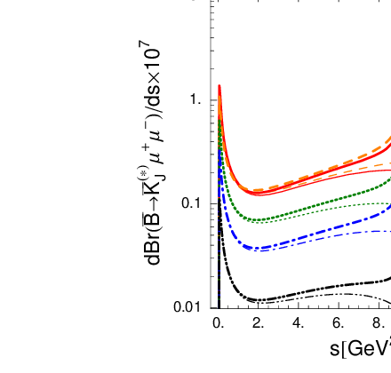
and θ\theta is the angle between the moving directions of ℓ+\ell^{+} and BB meson in the center of mass frame of the ℓ+​ℓ−\ell^{+}\ell^{-} pair. We show the decay distributions d​ℬ​(B¯0→K¯J(∗)​0​μ+​μ−)/d​sd{\cal B}(\overline{B}^{0}\to\overline{K}_{J}^{(*)0}\mu^{+}\mu^{-})/ds in Fig. 1 and summarize the corresponding branching fractions in Table 6. Because the decays involving heavier KK-resonances have the smaller phase spaces and LEET form factors and because the Clebsch-Gordan coefficients, αL(J)\alpha_{L}^{(J)} and βT(J)\beta_{T}^{(J)}, are smaller for a larger spin JJ, we obtain the following salient features:

ℬ⁡(B→K∗​(1410)​μ+​μ−)>ℬ⁡(B→K2∗​(1430)​μ+​μ−)>ℬ⁡(B→K∗​(1680)​μ+​μ−)\displaystyle{\cal B}(B\to K^{*}(1410)\mu^{+}\mu^{-})>{\cal B}(B\to K^{*}_{2}(1430)\mu^{+}\mu^{-})>{\cal B}(B\to K^{*}(1680)\mu^{+}\mu^{-})
>\displaystyle> ℬ⁡(B→K2∗​(1980)​μ+​μ−)≈ℬ⁡(B→K3∗​(1780)​μ+​μ−)>ℬ⁡(B→K4∗​(2045)​μ+​μ−)\displaystyle{\cal B}(B\to K^{*}_{2}(1980)\mu^{+}\mu^{-})\approx{\cal B}(B\to K^{*}_{3}(1780)\mu^{+}\mu^{-})>{\cal B}(B\to K^{*}_{4}(2045)\mu^{+}\mu^{-})
>\displaystyle> ℬ⁡(B→K5∗​(2380)​μ+​μ−),\displaystyle{\cal B}(B\to K^{*}_{5}(2380)\mu^{+}\mu^{-}), (74)

and

ℬ⁡(B→K1​(1650)​μ+​μ−)>ℬ⁡(B→K2​(1770)​μ+​μ−)>ℬ⁡(B→K2​(1820)​μ+​μ−)\displaystyle{\cal B}(B\to K_{1}(1650)\mu^{+}\mu^{-})>{\cal B}(B\to K_{2}(1770)\mu^{+}\mu^{-})>{\cal B}(B\to K_{2}(1820)\mu^{+}\mu^{-})
>\displaystyle> ℬ⁡(B→K2​(2250)​μ+​μ−)>ℬ⁡(B→K3​(2320)​μ+​μ−)>ℬ⁡(B→K4​(2500)​μ+​μ−)\displaystyle{\cal B}(B\to K_{2}(2250)\mu^{+}\mu^{-})>{\cal B}(B\to K_{3}(2320)\mu^{+}\mu^{-})>{\cal B}(B\to K_{4}(2500)\mu^{+}\mu^{-})
>\displaystyle> ℬ⁡(B→K5​(2600​?)​μ+​μ−).\displaystyle{\cal B}(B\to K_{5}(2600?)\mu^{+}\mu^{-}). (75)
Figure 1: Decay distributions of B¯0→K¯J(∗)​0​μ+​μ−\overline{B}^{0}\to\overline{K}_{J}^{(*)0}\mu^{+}\mu^{-} decays. The processes involving the confirmed KJ(∗)K_{J}^{(*)} are plotted. Solid [red], dashed [orange], dotted [green], dot-dashed [blue], and double-dot-dashed [black] curves from up to down correspond to KJ(∗)=K∗​(1680),K2∗​(1430),K2​(1770),K3∗​(1780)K_{J}^{(*)}=K^{*}({1680}),~K_{2}^{*}({1430}),K_{2}({1770}),~K_{3}^{*}({1780}), and K4∗​(2045)K_{4}^{*}({2045}), respectively. The thick and thin curves stand for the decay widths with and without charmonium resonances, respectively (see Eq. (69)).
Refer to caption
Table 6: Same as Table 5 except for nonresonant branching fractions of B¯→K¯J(∗)​μ+​μ−\overline{B}\to\overline{K}_{J}^{(*)}\mu^{+}\mu^{-} decays in units of 10−710^{-7}.
JP​CJ^{PC} n​LJ2​S+1n\,{}^{2S+1}L_{J} ℬ⁡(B¯0→K¯J(∗)​0​μ+​μ−){\cal B}(\overline{B}^{0}\to\overline{K}_{J}^{(*)0}\mu^{+}\mu^{-}) ℬ⁡(B−→KJ(∗)−​μ+​μ−){\cal B}(B^{-}\to K_{J}^{(*)-}\mu^{+}\mu^{-})
K∗​(1410)K^{*}({1410}) 1−⁣−1^{--} 2​S13{2}\,{}^{3}{S}_{1} 5.4+1.6−1.45.4{}^{+1.6}_{-1.4}{} 5.8+1.7−1.55.8{}^{+1.7}_{-1.5}{}
K∗​(1680)K^{*}({1680}) 1−⁣−1^{--} 1​D13{1}\,{}^{3}{D}_{1} 2.3+0.8−0.72.3{}^{+0.8}_{-0.7}{} 2.4+0.9−0.82.4{}^{+0.9}_{-0.8}{}
K2∗​(1430)K_{2}^{*}({1430}) 2+⁣+2^{++} 1​P23{1}\,{}^{3}{P}_{2} 3.1+0.9−0.83.1{}^{+0.9}_{-0.8}{} 3.3+1.0−0.93.3{}^{+1.0}_{-0.9}{}
K2∗​(1980)K_{2}^{*}({1980}) 2+?2^{+?} 1​F23{1}\,{}^{3}{F}_{2} or 2​P23{2}\,{}^{3}{P}_{2} 0.6+0.3−0.20.6{}^{+0.3}_{-0.2}{} 0.6+0.3−0.20.6{}^{+0.3}_{-0.2}{}
K3∗​(1780)K_{3}^{*}({1780}) 3−⁣−3^{--} 1​D33{1}\,{}^{3}{D}_{3} 0.6+0.2−0.20.6{}^{+0.2}_{-0.2}{} 0.6+0.2−0.20.6{}^{+0.2}_{-0.2}{}
K4∗​(2045)K_{4}^{*}({2045}) 4+⁣+4^{++} 1​F43{1}\,{}^{3}{F}_{4} 0.1+0.1−0.10.1{}^{+0.1}_{-0.1}{} 0.2+0.1−0.10.2{}^{+0.1}_{-0.1}{}
K5∗​(2380)K_{5}^{*}({2380}) 5−?5^{-?} 1​G53{1}\,{}^{3}{G}_{5} 0.03+0.02−0.010.03{}^{+0.02}_{-0.01}{} 0.03+0.02−0.010.03{}^{+0.02}_{-0.01}{}
K1​(1650)K_{1}({1650}) 1+?1^{+?} 2​P11{2}\,{}^{1}{P}_{1} or 2​P13{2}\,{}^{3}{P}_{1} 2.6+0.9−0.82.6{}^{+0.9}_{-0.8}{} 2.7+1.0−0.82.7{}^{+1.0}_{-0.8}{}
K2​(1770)K_{2}({1770}) 2−⁣+2^{-+} 1​D21{1}\,{}^{1}{D}_{2} 1.1+0.4−0.31.1{}^{+0.4}_{-0.3}{} 1.2+0.4−0.41.2{}^{+0.4}_{-0.4}{}
K2​(1820)K_{2}({1820}) 2−⁣−2^{--} 1​D23{1}\,{}^{3}{D}_{2}? 0.9+0.4−0.30.9{}^{+0.4}_{-0.3}{} 1.0+0.4−0.31.0{}^{+0.4}_{-0.3}{}
K2​(2250)K_{2}({2250}) 2−?2^{-?} 2​D21{2}\,{}^{1}{D}_{2} 0.2+0.1−0.10.2{}^{+0.1}_{-0.1}{} 0.2+0.1−0.10.2{}^{+0.1}_{-0.1}{}
K3​(2320)K_{3}({2320}) 3+?3^{+?} 1​F31{1}\,{}^{1}{F}_{3} or 1​F33{1}\,{}^{3}{F}_{3} 0.1+0.1−0.10.1{}^{+0.1}_{-0.1}{} 0.1+0.1−0.10.1{}^{+0.1}_{-0.1}{}
K4​(2500)K_{4}({2500}) 4−?4^{-?} 1​G41{1}\,{}^{1}{G}_{4} or 1​G43{1}\,{}^{3}{G}_{4} 0.03+0.02−0.020.03{}^{+0.02}_{-0.02}{} 0.03+0.02−0.020.03{}^{+0.02}_{-0.02}{}
K5​(2600​?)K_{5}({2600?}) 5+?5^{+?} 1​H51{1}\,{}^{1}{H}_{5} or 1​H53{1}\,{}^{3}{H}_{5}? 0.01+0.01−0.010.01{}^{+0.01}_{-0.01}{} 0.01+0.01−0.010.01{}^{+0.01}_{-0.01}{}
Total44 4 Same as Table 5. 19.9+6.2−4.619.9{}^{+6.2}_{-4.6}{} 21.4+7.1−5.221.4{}^{+7.1}_{-5.2}{}

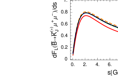
In Fig. 2, we plot the longitudinal fraction distributions for the B¯→K¯J(∗)​μ+​μ−\overline{B}\to\overline{K}_{J}^{(*)}\mu^{+}\mu^{-} decays, where

d​FLd​s≡d​ΓLd​s/d​Γtotald​s.\displaystyle\frac{dF_{L}}{ds}\equiv\frac{d\Gamma_{L}}{ds}\bigg/\frac{d\Gamma_{\rm total}}{ds}. (76)

Our result indicates that the longitudinal fraction distribution d​FL/d​sdF_{L}/ds about 0.80.8 at s=2​GeV2s=2\,{\rm GeV}^{2}, which also apply to the inclusive process. It is interesting to note that, for the new-physics models with the flipped sign solution for c7effc_{7}^{\rm eff}, d​FL/d​sdF_{L}/ds can be reduced to be ∼0.6\sim 0.6 at s=2​GeV2s=2\,{\rm GeV}^{2}.

Figure 2: Longitudinal fraction distributions d​FL/d​sdF_{L}/ds of B¯→K¯J(∗)​μ+​μ−\overline{B}\to\overline{K}_{J}^{(*)}\mu^{+}\mu^{-} decays as functions of ss. Solid [red], dashed [orange], dotted [green], dot-dashed [blue] and double-dot-dashed [black] curves stand for KJ(∗)=K∗​(1680)K_{J}^{(*)}=K^{*}({1680}), K2∗​(1430)K_{2}^{*}({1430}), K2​(1770)K_{2}({1770}), K3∗​(1780)K_{3}^{*}({1780}) and K4∗​(2045)K_{4}^{*}({2045}), respectively.
Refer to caption

The forward-backward asymmetry of B¯→K¯J∗​ℓ+​ℓ−\overline{B}\to\overline{K}_{J}^{*}\ell^{+}\ell^{-} is given by

d​AF​Bd​s^\displaystyle\frac{dA_{FB}}{d\hat{s}} =\displaystyle= −(βT(J))2GF2​αE​M2​mB5210​π5|Vt​s∗Vt​b|2s^u^(s)2[Re(ℬ(KJ∗)ℰ(KJ∗)∗)+Re(𝒜(KJ∗)ℱ(KJ∗)∗)]\displaystyle-\left(\beta_{T}^{(J)}{}\right)^{2}\frac{G_{F}^{2}\alpha_{EM}^{2}m_{B}^{5}}{2^{10}\pi^{5}}|V_{ts}^{*}V_{tb}|^{2}\hat{s}\hat{u}(s)^{2}\left[\mathop{\mbox{Re}}\left({\cal B}^{(K_{J}^{*})}{\cal E}^{(K_{J}^{*})*}\right)+\mathop{\mbox{Re}}\left({\cal A}^{(K_{J}^{*})}{\cal F}^{(K_{J}^{*})*}\right)\right] (77)
=\displaystyle= −(βT(J))2​GF2​αE​M2​mB5210​π5​|Vt​s∗​Vt​b|2​s^​u^​(s)2\displaystyle-\left(\beta_{T}^{(J)}{}\right)^{2}\frac{G_{F}^{2}\alpha_{EM}^{2}m_{B}^{5}}{2^{10}\pi^{5}}|V_{ts}^{*}V_{tb}|^{2}\hat{s}\hat{u}(s)^{2}
×[Re[c10c9eff(s^)]VKJ∗A1KJ∗\displaystyle\phantom{ii}\times\biggl[\mathop{\mbox{Re}}\left[c_{10}c_{9}^{{\rm eff}}(\hat{s})\right]V^{K_{J}^{*}}A_{1}^{K_{J}^{*}}
+m^bs^Re(c10c7eff){(1−m^KJ∗)VKJ∗T2KJ∗+(1+m^KJ∗)A1KJ∗T1KJ∗}].\displaystyle\phantom{MM}+\frac{\hat{m}_{b}}{\hat{s}}\mathop{\mbox{Re}}(c_{10}c_{7}^{{\rm eff}})\left\{(1-\hat{m}_{K_{J}^{*}})V^{K_{J}^{*}}T_{2}^{K_{J}^{*}}+(1+\hat{m}_{K_{J}^{*}})A_{1}^{K_{J}^{*}}T_{1}^{K_{J}^{*}}\right\}\biggr].

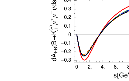
In Fig. 3 we plot the normalized forward-backward asymmetry d​A¯F​B/d​s≡(d​AF​B/d​s)/(d​Γtotal/d​s)d\bar{A}_{FB}/ds\equiv(dA_{FB}/ds)/(d\Gamma_{\rm total}/ds). Using the form factors in Eqs. (41)-(47), we can easily obtain the forward-backward asymmetry zero, s0s_{0}, satisfying

Re⁡[c9eff​(s^0)​c10]\displaystyle\mathop{\mbox{Re}}\left[c_{9}^{{\rm eff}}(\hat{s}_{0})c_{10}\right] =\displaystyle= −2m^bs^0Re(c7effc10)1−s^01+m^KJ(∗)2−s^0.\displaystyle-2\frac{\hat{m}_{b}}{\hat{s}_{0}}\mathop{\mbox{Re}}(c_{7}^{{\rm eff}}c_{10})\frac{1-\hat{s}_{0}}{1+\hat{m}_{K_{J}^{(*)}}^{2}-\hat{s}_{0}}. (78)

We note that s0s_{0} is independent of the form factors but depends only on mKJ(∗)m_{K_{J}^{(*)}}. Under the variation of m^KJ(∗)2\hat{m}_{K_{J}^{(*)}}^{2}, we get

δ​s^0≃(s^0−1)​s^0(s^0−1)2+m^KJ(∗)2​δ​m^KJ(∗)2,\displaystyle\delta\hat{s}_{0}\simeq\frac{(\hat{s}_{0}-1)\hat{s}_{0}}{(\hat{s}_{0}-1)^{2}+\hat{m}_{K_{J}^{(*)}}^{2}}\delta\hat{m}_{K_{J}^{(*)}}^{2}, (79)

or

δ​s0\displaystyle\delta s_{0} ≃\displaystyle\simeq −s0⋅δ​mKJ(∗)2mB2.\displaystyle-s_{0}\cdot\frac{\delta m_{K_{J}^{(*)}}^{2}}{m_{B}^{2}}. (80)

Since δ​mKJ(∗)2≪s0\delta m_{K_{J}^{(*)}}^{2}\ll s_{0} and mKJ(∗)2≪mB2m_{K_{J}^{(*)}}^{2}\ll m_{B}^{2}, we thus expect the following relation in the SM:
s0K∗​(980)≈3.5​GeV2⪆s0K∗​(1410)⪆s0K2∗​(1430)⪆s0K∗​(1680)⪆s0K2​(1770)⪆s0K3∗​(1780)⪆s0K2​(1820)\displaystyle s_{0}^{K^{*}(980)}\approx 3.5\,{\rm GeV}^{2}\gtrapprox s_{0}^{K^{*}({1410})}\gtrapprox s_{0}^{K_{2}^{*}({1430})}\gtrapprox s_{0}^{K^{*}({1680})}\gtrapprox s_{0}^{K_{2}({1770})}\gtrapprox s_{0}^{K_{3}^{*}({1780})}\gtrapprox s_{0}^{K_{2}({1820})}
⪆s0K2∗​(1980)⪆s0K4∗​(2045)⪆s0K2​(2250)⪆s0K3​(2320)⪆s0K5∗​(2380)⪆s0K4​(2500)⪆s0K5​(2600​?).\displaystyle\gtrapprox s_{0}^{K_{2}^{*}({1980})}\gtrapprox s_{0}^{K_{4}^{*}({2045})}\gtrapprox s_{0}^{K_{2}({2250})}\gtrapprox s_{0}^{K_{3}({2320})}\gtrapprox s_{0}^{K_{5}^{*}({2380})}\gtrapprox s_{0}^{K_{4}({2500})}\gtrapprox s_{0}^{K_{5}({2600?})}.
Figure 3: Normalized forward-backward asymmetries for B¯→K¯J(∗)​μ+​μ−\overline{B}\to\overline{K}_{J}^{(*)}\mu^{+}\mu^{-} decay. Legends are the same as Fig. 2.
Refer to caption

III.3 B¯→K¯J(∗)​ν​ν¯\overline{B}\to\overline{K}_{J}^{(*)}\nu\bar{\nu} Decays

The effective weak Hamiltonian relevant to the B¯→K¯J(∗)​ν​ν¯\overline{B}\to\overline{K}_{J}^{(*)}\nu\bar{\nu} decays are given by

ℋeff=cL​s¯​γμ​(1−γ5)​b​ν¯​γμ​(1−γ5)​ν+cR​s¯​γμ​(1+γ5)​b​ν¯​γμ​(1−γ5)​ν+H.c.,\displaystyle{\cal H}_{{\rm eff}}=c_{L}\bar{s}\gamma^{\mu}(1-\gamma_{5})b\,\bar{\nu}\gamma_{\mu}(1-\gamma_{5})\nu+c_{R}\bar{s}\gamma^{\mu}(1+\gamma_{5})b\,\bar{\nu}\gamma_{\mu}(1-\gamma_{5})\nu+\mbox{H.c.}, (82)

where cLc_{L} and cRc_{R} are coefficients for left- and right-handed weak hadronic currents, respectively. In the SM, cRS​M=0c_{R}^{SM}=0 and

cLS​M\displaystyle c_{L}^{SM} =\displaystyle= GF2​αE​M2​π​sin2⁡θW​Vt​b​Vt​s∗​X​(xt)=2.9×10⁻⁹,\displaystyle\frac{G_{F}}{\sqrt{2}}\frac{\alpha_{EM}}{2\pi\sin^{2}\theta_{W}}V_{tb}V_{ts}^{*}X(x_{t})=2.9\times 10^{-9}, (83)

where the detailed form of X⁡(xt)X(x_{t}) has been given in Refs. [44, 45]. The missing invariant mass-squared distributions, corresponding to polarizations h=0,±1h=0,\pm 1 of the final K¯J∗\overline{K}_{J}^{*} for B¯→K¯J∗​ν​ν¯\overline{B}\to\overline{K}_{J}^{*}\nu\bar{\nu} decays are55 5 For the amplitudes of B¯→K¯J​ν​ν¯\overline{B}\to\overline{K}_{J}\nu\bar{\nu} decays, perform the following replacements: VKJ∗→AKJV^{K_{J}^{*}}\to A^{K_{J}}, AiKJ∗→ViKJA_{i}^{K_{J}^{*}}\to V_{i}^{K_{J}}.,

d​Γ0d​q2\displaystyle\frac{d\Gamma_{0}}{dq^{2}} =\displaystyle= 3​(αL(J))2​|p→′|48​π3​|cL−cR|2mKJ∗2\displaystyle 3\left(\alpha_{L}^{(J)}{}\right)^{2}\frac{|\vec{p}^{\prime}|}{48\pi^{3}}\frac{|c_{L}-c_{R}|^{2}}{m_{K_{J}^{*}}^{2}} (84)
×[(mB+mKJ∗)​(mB​E′−mKJ∗2)​A1KJ∗​(q2)−2​mB2mB+mKJ∗​|p→′|2​A2KJ∗​(q2)]2,\displaystyle\times\left[(m_{B}+m_{K_{J}^{*}})(m_{B}E^{\prime}-m_{K_{J}^{*}}^{2})A_{1}^{K_{J}^{*}}(q^{2})-\frac{2m_{B}^{2}}{m_{B}+m_{K_{J}^{*}}}|\vec{p}^{\prime}|^{2}A_{2}^{K_{J}^{*}}(q^{2})\right]^{2},
d​Γ±1d​q2\displaystyle\frac{d\Gamma_{\pm 1}}{dq^{2}} =\displaystyle= 3​(βT(J))2​|p→′|​q248​π3\displaystyle 3\left(\beta_{T}^{(J)}{}\right)^{2}\frac{|\vec{p}^{\prime}|q^{2}}{48\pi^{3}} (85)
×|(cL+cR)​2​mB​|p→′|mB+mKJ∗​VKJ∗​(q2)∓(cL−cR)​(mB+mKJ∗)​A1KJ∗​(q2)|2,\displaystyle\times\Biggl|(c_{L}+c_{R})\frac{2m_{B}|\vec{p}^{\prime}|}{m_{B}+m_{K_{J}^{*}}}V^{K_{J}^{*}}(q^{2})\mp(c_{L}-c_{R})(m_{B}+m_{K_{J}^{*}})A_{1}^{K_{J}^{*}}(q^{2})\Biggr|^{2},

where the factor 33 counts the numbers of the neutrino generations, (E′,p→′)(E^{\prime},\vec{p}^{\prime}) is the K¯J∗\overline{K}_{J}^{*} energy-momentum in the BB-meson rest frame, and q2q^{2} is the invariant mass squared of the neutrino-antineutrino pair with 0≤q2≤(mB−mKJ∗)20\leq q^{2}\leq(m_{B}-m_{K_{J}^{*}})^{2}. In Fig. 4, we show the differential distributions as functions of the missing invariant mass squared in the SM. The results for branching fractions are summarized in Table 7. At q2=0q^{2}=0, where the neutrino and antineutrino are nearly collinear in the BB rest frame, the decay is predominated by the zero helicity amplitude. Moreover, as expected from the left-handed bL→sLb_{L}\to s_{L} transition in the SM, d​Γ+/d​q2d\Gamma_{+}/dq^{2} is always suppressed at least by (ms/mb)2(m_{s}/m_{b})^{2}, compared with d​Γ0/d​q2d\Gamma_{0}/dq^{2} and d​Γ−/d​q2d\Gamma_{-}/dq^{2}. We obtain the relation: d​Γ0/d​q2>d​Γ−/d​q2≫d​Γ+/d​q2d\Gamma_{0}/dq^{2}>d\Gamma_{-}/dq^{2}\gg d\Gamma_{+}/dq^{2}.

Figure 4: The d​ℬ​(B¯→K¯J(∗)​ν​ν¯)/d​q2d{\cal B}(\overline{B}\to\overline{K}_{J}^{(*)}\nu\bar{\nu})/dq^{2} as functions of the missing invariant mass-squared q2q^{2}. The solid [black], dashed [blue], dotted [green] and dot-dashed [red] curves correspond to the total decay rate and the polarization rates with helicities h=0,−1,+1h=0,-1,+1, respectively.
Refer to caption
Refer to caption
Refer to caption
Refer to caption
Table 7: The branching fractions of the B→KJ(∗)​ν​ν¯B\to K_{J}^{(*)}\nu\bar{\nu} decays in units of 10−610^{-6}. The first and second errors correspond to the uncertainties of the form factors ζ⟂KJ(∗)\zeta_{\perp}^{K_{J}^{(*)}} and ξKJ(∗)\xi^{K_{J}^{(*)}}, respectively.
JP​CJ^{PC} n​LJ2​S+1{n}\,{}^{2S+1}{L}_{J} ℬ⁡(B¯0→K¯J(∗)​0​ν​ν¯){\cal B}(\overline{B}^{0}\to\overline{K}_{J}^{(*)0}\nu\bar{\nu}) ℬ⁡(B−→KJ(∗)−​ν​ν¯){\cal B}(B^{-}\to K_{J}^{(*)-}\nu\bar{\nu})
K∗​(1410)K^{*}({1410}) 1−⁣−1^{--} 2​S13{2}\,{}^{3}{S}_{1}? 4.3+1.3−1.14.3{}^{+1.3}_{-1.1}{} 4.6+1.4−1.24.6{}^{+1.4}_{-1.2}{}
K∗​(1680)K^{*}({1680}) 1−⁣−1^{--} 1​D13{1}\,{}^{3}{D}_{1} 1.8+0.7−0.61.8{}^{+0.7}_{-0.6}{} 2.0+0.7−0.62.0{}^{+0.7}_{-0.6}{}
K2∗​(1430)K_{2}^{*}({1430}) 2+⁣+2^{++} 1​P23{1}\,{}^{3}{P}_{2} 2.5+0.7−0.62.5{}^{+0.7}_{-0.6}{} 2.6+0.8−0.72.6{}^{+0.8}_{-0.7}{}
K2∗​(1980)K_{2}^{*}({1980}) 2+?2^{+?} 1​F23{1}\,{}^{3}{F}_{2} or 2​P23{2}\,{}^{3}{P}_{2}? 0.4+0.2−0.20.4{}^{+0.2}_{-0.2}{} 0.5+0.2−0.20.5{}^{+0.2}_{-0.2}{}
K3∗​(1780)K_{3}^{*}({1780}) 3−⁣−3^{--} 1​D33{1}\,{}^{3}{D}_{3} 0.5+0.2−0.20.5{}^{+0.2}_{-0.2}{} 0.5+0.2−0.20.5{}^{+0.2}_{-0.2}{}
K4∗​(2045)K_{4}^{*}({2045}) 4+⁣+4^{++} 1​F43{1}\,{}^{3}{F}_{4} 0.11+0.05−0.040.11{}^{+0.05}_{-0.04}{} 0.11+0.06−0.050.11{}^{+0.06}_{-0.05}{}
K5∗​(2380)K_{5}^{*}({2380}) 5−?5^{-?} 1​G53{1}\,{}^{3}{G}_{5} 0.02+0.01−0.010.02{}^{+0.01}_{-0.01}{} 0.02+0.01−0.010.02{}^{+0.01}_{-0.01}{}
K1​(1650)K_{1}({1650}) 1+?1^{+?} 2​P11{2}\,{}^{1}{P}_{1} or 2​P13{2}\,{}^{3}{P}_{1}? 2.1+0.7−0.62.1{}^{+0.7}_{-0.6}{} 2.2+0.8−0.72.2{}^{+0.8}_{-0.7}{}
K2​(1770)K_{2}({1770}) 2−⁣+2^{-+} 1​D21{1}\,{}^{1}{D}_{2} 0.9+0.3−0.30.9{}^{+0.3}_{-0.3}{} 0.9+0.4−0.30.9{}^{+0.4}_{-0.3}{}
K2​(1820)K_{2}({1820}) 2−⁣−2^{--} 1​D23{1}\,{}^{3}{D}_{2}? 0.7+0.3−0.20.7{}^{+0.3}_{-0.2}{} 0.8+0.3−0.30.8{}^{+0.3}_{-0.3}{}
K2​(2250)K_{2}({2250}) 2−?2^{-?} 2​D21{2}\,{}^{1}{D}_{2} 0.2+0.1−0.10.2{}^{+0.1}_{-0.1}{} 0.2+0.1−0.10.2{}^{+0.1}_{-0.1}{}
K3​(2320)K_{3}({2320}) 3+?3^{+?} 1​F31{1}\,{}^{1}{F}_{3} or 1​F33{1}\,{}^{3}{F}_{3} 0.07+0.05−0.030.07{}^{+0.05}_{-0.03}{} 0.07+0.05−0.040.07{}^{+0.05}_{-0.04}{}
K4​(2500)K_{4}({2500}) 4−?4^{-?} 1​G41{1}\,{}^{1}{G}_{4} or 1​G43{1}\,{}^{3}{G}_{4} 0.02+0.02−0.010.02{}^{+0.02}_{-0.01}{} 0.02+0.01−0.010.02{}^{+0.01}_{-0.01}{}
K5​(2600)K_{5}({2600}) 5+?5^{+?} 1​H51{1}\,{}^{1}{H}_{5} or 1​H53{1}\,{}^{3}{H}_{5} 0.008+0.006−0.0050.008{}^{+0.006}_{-0.005}{} 0.008+0.007−0.0050.008{}^{+0.007}_{-0.005}{}
Total66 6 Same as Table 5. 16.2+4.1−3.016.2{}^{+4.1}_{-3.0}{} 17.3+4.7−3.517.3{}^{+4.7}_{-3.5}{}

IV Summary

We have formulated B→KJ(∗)B\to K_{J}^{(*)} form factors using large energy effective theory techniques. We have studied the radiative and semileptonic BB decays involving the higher strange resonance KJ(∗)K_{J}^{(*)} in the final state. The main results are as follows.

  • •

    The transition form factors in the large recoil region can be represented in terms of two independent LEET form factors, ζ⟂KJ(∗)​(q2)\zeta^{K_{J}^{(*)}}_{\perp}(q^{2}) and ζ∥KJ(∗)​(q2)\zeta^{K_{J}^{(*)}}_{\parallel}(q^{2}). According to the QCD counting rules, these two form factors exhibit the dipole q2q^{2} dependence in the large recoil region (and in the LEET limit). We have further estimated ζ⟂KJ(∗)​(0)\zeta^{K_{J}^{(*)}}_{\perp}(0) and ζ∥KJ(∗)​(0)\zeta^{K_{J}^{(*)}}_{\parallel}(0) in the BSW model.

  • •

    The branching fractions for decays B¯→K¯J(∗)​γ\overline{B}\to\overline{K}_{J}^{(*)}\gamma, B¯→K¯J(∗)​ℓ+​ℓ−\overline{B}\to\overline{K}_{J}^{(*)}\ell^{+}\ell^{-} and B¯→K¯J(∗)​ν​ν¯\overline{B}\to\overline{K}_{J}^{(*)}\nu\bar{\nu} with higher KK-resonances are suppressed due to the smaller phase space and ζKJ(∗)⟂,∥\zeta^{K_{J}^{(*)}}_{\perp,\parallel}, and/or due to the smaller Clebsch-Gordan coefficients, βT(J)\beta_{T}^{(J)}{} and αL(J)\alpha_{L}^{(J)}{}, in case of larger spin-JJ.

  • •

    We find that for B¯→K¯J(∗)​ℓ+​ℓ−\overline{B}\to\overline{K}_{J}^{(*)}\ell^{+}\ell^{-} decays, the longitudinal fraction distribution d​FL/d​s≃0.8dF_{L}/ds\simeq 0.8 at s=2​GeV2s=2\,{\rm GeV}^{2}, and the forward-backward asymmetry zero s0≈3.5​GeV2s_{0}\approx 3.5\,{\rm GeV}^{2}. The asymmetry zero is independent of the form factors in the LEET limit and highly insensitive to mKJ(∗)m_{K_{J}^{(*)}}.

  • •

    For the B¯→K¯J(∗)​ν​ν¯\overline{B}\to\overline{K}_{J}^{(*)}\nu\bar{\nu} decay, the branching fraction is predominated by the zero helicity amplitude at q2=0q^{2}=0, where the neutrino and antineutrino are nearly collinear in the BB rest frame. As expected from the left-handed bL→sLb_{L}\to s_{L} current in the SM, d​Γ+/d​q2d\Gamma_{+}/dq^{2} is always suppressed at least by (ms/mb)2(m_{s}/m_{b})^{2}, compared with d​Γ0/d​q2d\Gamma_{0}/dq^{2} and d​Γ−/d​q2d\Gamma_{-}/dq^{2}. We thus predict the relation: d​Γ0/d​q2>d​Γ−/d​q2≫d​Γ+/d​q2d\Gamma_{0}/dq^{2}>d\Gamma_{-}/dq^{2}\gg d\Gamma_{+}/dq^{2}.

Acknowledgements.
This research was supported in parts by the National Science Council of R.O.C. under Grant No. NSC96-2112-M-033-004-MY3 and No. NSC97-2811-033-003 and by the National Center for Theoretical Science.

Appendix A B¯→K¯J\overline{B}\to\overline{K}_{J} form factors

B¯→K¯J\overline{B}\to\overline{K}_{J} transition form factors in the LEET limit are given by

⟨K¯J|Aμ|B¯⟩\displaystyle{\langle{\overline{K}_{J}}}|A^{\mu}|{{\overline{B}}\rangle} =\displaystyle= −i​2​E​(mKJE)J−1​ζ⟂KJ​(a)​ϵμ​ν​ρ​σ​vν​nρ​eσ∗,\displaystyle-i2E\left(\frac{m_{K_{J}}}{E}\right)^{J-1}\zeta^{K_{J}(a)}_{\perp}\epsilon^{\mu\nu\rho\sigma}v_{\nu}n_{\rho}e^{*}_{\sigma}, (86)
⟨K¯J|Vμ|B¯⟩\displaystyle{\langle{\overline{K}_{J}}}|V^{\mu}|{{\overline{B}}\rangle} =\displaystyle= 2​E​(mKJE)J−1​ζ⟂KJ​(v)​[e∗μ−(e∗⋅v)​nμ]\displaystyle 2E\left(\frac{m_{K_{J}}}{E}\right)^{J-1}\zeta^{K_{J}(v)}_{\perp}\left[e^{*\mu}-(e^{*}\cdot v)n^{\mu}\right] (87)
+2E(mKJE)J(e∗⋅v)[ζ∥KJ​(v)nμ+ζ∥,1KJ​(v)vμ],\displaystyle+2E\left(\frac{m_{K_{J}}}{E}\right)^{J}(e^{*}\cdot v)\left[\zeta^{K_{J}(v)}_{\parallel}n^{\mu}+\zeta^{K_{J}(v)}_{\parallel,1}v^{\mu}\right],
⟨K¯J|TAμ​ν|B¯⟩\displaystyle{\langle{\overline{K}_{J}}}|T_{A}^{\mu\nu}|{{\overline{B}}\rangle} =\displaystyle= −2​E​(mKJE)J​ζ∥KJ​(t5)​(e∗⋅v)​ϵμ​ν​ρ​σ​vρ​nσ\displaystyle-2E\left(\frac{m_{K_{J}}}{E}\right)^{J}\zeta^{K_{J}(t_{5})}_{\parallel}(e^{*}\cdot v)\epsilon^{\mu\nu\rho\sigma}v_{\rho}n_{\sigma} (88)
−2​E​(mKJE)J−1​ζ⟂KJ​(t5)​ϵμ​ν​ρ​σ​nρ​[eσ∗−(e∗⋅v)​nσ]\displaystyle-2E\left(\frac{m_{K_{J}}}{E}\right)^{J-1}\zeta^{K_{J}(t_{5})}_{\perp}\epsilon^{\mu\nu\rho\sigma}n_{\rho}[e^{*}_{\sigma}-(e^{*}\cdot v)n_{\sigma}]
−2​E​(mKJE)J−1​ζ⟂,1KJ​(t5)​ϵμ​ν​ρ​σ​vρ​[eσ∗−(e∗⋅v)​nσ],\displaystyle-2E\left(\frac{m_{K_{J}}}{E}\right)^{J-1}\zeta^{K_{J}(t_{5})}_{\perp,1}\epsilon^{\mu\nu\rho\sigma}v_{\rho}[e^{*}_{\sigma}-(e^{*}\cdot v)n_{\sigma}],
⟨K¯J|Tμ​ν|B¯⟩\displaystyle{\langle{\overline{K}_{J}}}|T^{\mu\nu}|{{\overline{B}}\rangle} =\displaystyle= i​2​E​(mKJE)J−1​ζ⟂,1KJ​(t)​{[e∗μ−(e∗⋅v)​nμ]​vν−(μ↔ν)}\displaystyle i2E\left(\frac{m_{K_{J}}}{E}\right)^{J-1}\zeta^{K_{J}(t)}_{\perp,1}\left\{\left[e^{*\mu}-(e^{*}\cdot v)n^{\mu}\right]v^{\nu}-(\mu\leftrightarrow\nu)\right\} (89)
+i​2​E​(mKJE)J−1​ζ⟂KJ​(t)​{[e∗μ−(e∗⋅v)​nμ]​nν−(μ↔ν)}\displaystyle+i2E\left(\frac{m_{K_{J}}}{E}\right)^{J-1}\zeta^{K_{J}(t)}_{\perp}\left\{[e^{*\mu}-(e^{*}\cdot v)n^{\mu}]n^{\nu}-(\mu\leftrightarrow\nu)\right\}
+i​2​E​(mKJE)J​ζ∥KJ​(t)​(e∗⋅v)​(nμ​vν−nν​vμ),\displaystyle+i2E\left(\frac{m_{K_{J}}}{E}\right)^{J}\zeta^{K_{J}(t)}_{\parallel}(e^{*}\cdot v)(n^{\mu}v^{\nu}-n^{\nu}v^{\mu}),

where mKJm_{K_{J}} is the mass of the KJK_{J}. ⟨K¯J|TAμ​ν|B¯⟩{\langle{\overline{K}_{J}}}|T_{A}^{\mu\nu}|{{\overline{B}}\rangle} is related to ⟨K¯J|Tμ​ν|B¯⟩{\langle{\overline{K}_{J}}}|T^{\mu\nu}|{{\overline{B}}\rangle} by the relation: σμ​ν​ϵμ​ν​ρ​σ=2​i​σρ​σ​γ5\sigma^{\mu\nu}\epsilon_{\mu\nu\rho\sigma}=2i\sigma^{\rho\sigma}\gamma_{5}. From operator relations Eqs. (28)-(32) and

s¯n​γ5​bv\displaystyle\bar{s}_{n}\gamma_{5}b_{v} =\displaystyle= −nμ​s¯n​γμ​γ5​bv,\displaystyle-n_{\mu}\bar{s}_{n}\gamma^{\mu}\gamma_{5}b_{v}, (90)

we obtain

ζ⟂KJ​(v)=ζ⟂KJ​(a)=ζ⟂KJ​(t)=ζ⟂KJ​(t5)\displaystyle\zeta^{K_{J}(v)}_{\perp}=\zeta^{K_{J}(a)}_{\perp}=\zeta^{K_{J}(t)}_{\perp}=\zeta^{K_{J}(t_{5})}_{\perp} ≡\displaystyle\equiv ζ⟂KJ,\displaystyle\zeta^{K_{J}}_{\perp}, (91)
ζ∥KJ​(a)=ζ∥KJ​(t)=ζ∥KJ​(t5)\displaystyle\zeta^{K_{J}(a)}_{\parallel}=\zeta^{K_{J}(t)}_{\parallel}=\zeta^{K_{J}(t_{5})}_{\parallel} ≡\displaystyle\equiv ζ∥KJ,\displaystyle\zeta^{K_{J}}_{\parallel}, (92)
ζKJ​(a)∥,1=ζKJ​(t5)⟂,1=ζKJ​(t)⟂,1\displaystyle\zeta^{K_{J}(a)}_{\parallel,1}=\zeta^{K_{J}(t_{5})}_{\perp,1}=\zeta^{K_{J}(t)}_{\perp,1} =\displaystyle= 0,\displaystyle 0, (93)

and thus find that there are only two independent form factors, ζ⟂KJ​(q2)\zeta^{K_{J}}_{\perp}(q^{2}) and ζ∥KJ​(q2)\zeta^{K_{J}}_{\parallel}(q^{2}).

B¯→K¯J\overline{B}\to\overline{K}_{J} form factors are given by

⟨K¯J​(pKJ,λ)|s¯​γμ​γ5​b|B¯​(pB)⟩\displaystyle{\langle{\overline{K}_{J}(p_{K_{J}},\lambda)}}|\bar{s}\gamma^{\mu}\gamma_{5}b|{{\overline{B}(p_{B})}\rangle} =\displaystyle= −i​2mB+mKJ​A~KJ​(q2)​ϵμ​ν​ρ​σ​pB​ν​pKJ​ρ​e​(λ)σ∗,\displaystyle-i\frac{2}{m_{B}+m_{K_{J}}}\tilde{A}^{K_{J}}(q^{2})\epsilon^{\mu\nu\rho\sigma}p_{B\nu}p_{K_{J}\rho}e(\lambda)_{\sigma}^{*}, (94)
⟨K¯J​(pKJ,λ)|s¯​γμ​b|B¯​(pB)⟩\displaystyle{\langle{\overline{K}_{J}(p_{K_{J}},\lambda)}}|\bar{s}\gamma^{\mu}b|{{\overline{B}(p_{B})}\rangle} =\displaystyle= 2​mKJ​V~0KJ​(q2)​e​(λ)∗⋅pBq2​qμ\displaystyle 2m_{K_{J}}\tilde{V}_{0}^{K_{J}}(q^{2})\frac{e(\lambda)^{*}\cdot p_{B}}{q^{2}}q^{\mu} (95)
+(mB+mKJ)​V~1KJ​(q2)​[e​(λ)∗μ−e​(λ)∗⋅pBq2​qμ]\displaystyle+\left(m_{B}+m_{K_{J}}\right)\tilde{V}_{1}^{K_{J}}(q^{2})\left[e(\lambda)^{*\mu}-\frac{e(\lambda)^{*}\cdot p_{B}}{q^{2}}q^{\mu}\right]
−V~2KJ​(q2)​e​(λ)∗⋅pBmB+mKJ​[pBμ+pKJμ−mB2−mKJ2q2​qμ],\displaystyle-\tilde{V}_{2}^{K_{J}}(q^{2})\frac{e(\lambda)^{*}\cdot p_{B}}{m_{B}+m_{K_{J}}}\left[p_{B}^{\mu}+p_{K_{J}}^{\mu}-\frac{m_{B}^{2}-m_{K_{J}}^{2}}{q^{2}}q^{\mu}\right],
⟨K¯J​(pKJ,λ)|s¯​σμ​ν​γ5​qν​b|B¯​(pB)⟩\displaystyle{\langle{\overline{K}_{J}(p_{K_{J}},\lambda)}}|\bar{s}\sigma^{\mu\nu}\gamma_{5}q_{\nu}b|{{\overline{B}(p_{B})}\rangle} =\displaystyle= 2​T~1KJ​(q2)​ϵμ​ν​ρ​σ​pB​ν​pKJ​ρ​e​(λ)σ∗,\displaystyle 2\tilde{T}_{1}^{K_{J}}(q^{2})\epsilon^{\mu\nu\rho\sigma}p_{B\nu}p_{K_{J}\rho}e(\lambda)^{*}_{\sigma}, (96)
⟨K¯J​(pKJ∗,λ)|s¯​σμ​ν​qν​b|B¯​(pB)⟩\displaystyle{\langle{\overline{K}_{J}(p_{K_{J}^{*}},\lambda)}}|\bar{s}\sigma^{\mu\nu}q_{\nu}b|{{\overline{B}(p_{B})}\rangle} =\displaystyle= i​T~2KJ​(q2)​[(mB2−mKJ2)​e​(λ)∗μ−(e​(λ)∗⋅pB)​(pBμ+pKJμ)]\displaystyle i\tilde{T}_{2}^{K_{J}}(q^{2})\left[\left(m_{B}^{2}-m_{K_{J}}^{2}\right)e(\lambda)^{*\mu}-\left(e(\lambda)^{*}\cdot p_{B}\right)\left(p_{B}^{\mu}+p_{K_{J}}^{\mu}\right)\right] (97)
+i​T~3KJ​(q2)​(e​(λ)∗⋅pB)\displaystyle+i\tilde{T}_{3}^{K_{J}}(q^{2})\left(e(\lambda)^{*}\cdot p_{B}\right)
×[qμ−q2mB2−mKJ2​(pBμ+pKJμ)].\displaystyle\phantom{MMM}\times\left[q^{\mu}-\frac{q^{2}}{m_{B}^{2}-m_{K_{J}}^{2}}\left(p_{B}^{\mu}+p_{K_{J}}^{\mu}\right)\right].

We can further obtain the following relations,

V~0KJ​(q2)​(|p→KJ|mKJ)J−1≡V0KJ​(q2)\displaystyle\tilde{V}_{0}^{K_{J}}(q^{2})\left(\frac{|\vec{p}_{K_{J}}|}{m_{K_{J}}}\right)^{J-1}\equiv V_{0}^{K_{J}}(q^{2}) ≃\displaystyle\simeq (1−mKJ2mB​E)​ζ∥KJ​(q2)+mKJmB​ζ⟂KJ​(q2),\displaystyle\left(1-\frac{m_{K_{J}}^{2}}{m_{B}E}\right)\zeta_{\parallel}^{K_{J}}(q^{2})+\frac{m_{K_{J}}}{m_{B}}\zeta_{\perp}^{K_{J}}(q^{2}), (98)
V~1KJ​(q2)​(|p→KJ|mKJ)J−1≡V1KJ​(q2)\displaystyle\tilde{V}_{1}^{K_{J}}(q^{2})\left(\frac{|\vec{p}_{K_{J}}|}{m_{K_{J}}}\right)^{J-1}\equiv V_{1}^{K_{J}}(q^{2}) ≃\displaystyle\simeq 2​EmB+mKJ​ζ⟂KJ​(q2),\displaystyle\frac{2E}{m_{B}+m_{K_{J}}}\zeta_{\perp}^{K_{J}}(q^{2}), (99)
V~2KJ​(q2)​(|p→KJ|mKJ)J−1≡V2KJ​(q2)\displaystyle\tilde{V}_{2}^{K_{J}}(q^{2})\left(\frac{|\vec{p}_{K_{J}}|}{m_{K_{J}}}\right)^{J-1}\equiv V_{2}^{K_{J}}(q^{2}) ≃\displaystyle\simeq (1+mKJmB)​[ζ⟂KJ​(q2)−mKJE​ζ∥KJ​(q2)],\displaystyle\left(1+\frac{m_{K_{J}}}{m_{B}}\right)\left[\zeta_{\perp}^{K_{J}}(q^{2})-\frac{m_{K_{J}}}{E}\zeta_{\parallel}^{K_{J}}(q^{2})\right], (100)
A~KJ​(q2)​(|p→KJ|mKJ)J−1≡AKJ​(q2)\displaystyle\tilde{A}^{K_{J}}(q^{2})\left(\frac{|\vec{p}_{K_{J}}|}{m_{K_{J}}}\right)^{J-1}\equiv A^{K_{J}}(q^{2}) ≃\displaystyle\simeq (1+mKJmB)​ζ⟂KJ​(q2),\displaystyle\left(1+\frac{m_{K_{J}}}{m_{B}}\right)\zeta_{\perp}^{K_{J}}(q^{2}), (101)
T~1KJ​(q2)​(|p→KJ|mKJ)J−1≡T1KJ​(q2)\displaystyle\tilde{T}_{1}^{K_{J}}(q^{2})\left(\frac{|\vec{p}_{K_{J}}|}{m_{K_{J}}}\right)^{J-1}\equiv T_{1}^{K_{J}}(q^{2}) ≃\displaystyle\simeq ζ⟂KJ​(q2),\displaystyle\zeta_{\perp}^{K_{J}}(q^{2}), (102)
T~2KJ​(q2)​(|p→KJ|mKJ)J−1≡T2KJ​(q2)\displaystyle\tilde{T}_{2}^{K_{J}}(q^{2})\left(\frac{|\vec{p}_{K_{J}}|}{m_{K_{J}}}\right)^{J-1}\equiv T_{2}^{K_{J}}(q^{2}) ≃\displaystyle\simeq (1−q2mB2−mKJ2)​ζ⟂KJ​(q2),\displaystyle\left(1-\frac{q^{2}}{m_{B}^{2}-m_{K_{J}}^{2}}\right)\zeta_{\perp}^{K_{J}}(q^{2}), (103)
T~3KJ​(q2)​(|p→KJ|mKJ)J−1≡T3KJ​(q2)\displaystyle\tilde{T}_{3}^{K_{J}}(q^{2})\left(\frac{|\vec{p}_{K_{J}}|}{m_{K_{J}}}\right)^{J-1}\equiv T_{3}^{K_{J}}(q^{2}) ≃\displaystyle\simeq ζ⟂KJ​(q2)−(1−mKJ2mB2)​mKJE​ζ∥KJ​(q2),\displaystyle\zeta_{\perp}^{K_{J}}(q^{2})-\left(1-\frac{m_{K_{J}}^{2}}{m_{B}^{2}}\right)\frac{m_{K_{J}}}{E}\zeta_{\parallel}^{K_{J}}(q^{2}), (104)

where use of p3/E≃1p_{3}/E\simeq 1 has been made. Recalling that

ε~(J)​(0)μ=αL(J)​ε​(0)μ,ε~(J)​(±1)μ=βT(J)​ε​(±1)μ,\displaystyle\tilde{\varepsilon}_{(J)}{}(0)^{\mu}=\alpha_{L}^{(J)}{}\varepsilon(0)^{\mu},\quad\tilde{\varepsilon}_{(J)}{}(\pm 1)^{\mu}=\beta_{T}^{(J)}{}\varepsilon(\pm 1)^{\mu}, (105)

we can easily generalize the studies for B→KJ∗​γB\to K_{J}^{*}\gamma, B→KJ∗​ℓ+​ℓ−B\to K_{J}^{*}\ell^{+}\ell^{-} and B→KJ∗​ν​ν¯B\to K_{J}^{*}\nu\bar{\nu} to B→KJ​γB\to K_{J}\gamma, B→KJ​ℓ+​ℓ−B\to K_{J}\ell^{+}\ell^{-} and B→KJ​ν​ν¯B\to K_{J}\nu\bar{\nu} by the following replacements:

VKJ∗→AKJ,AiKJ∗→ViKJ(i=0,1,2),TjKJ∗→TjKJ(j=1,2,3).\displaystyle V^{K_{J}^{*}}\to A^{K_{J}},\quad A_{i}^{K_{J}^{*}}\to V_{i}^{K_{J}}\quad(i=0,1,2),\quad T_{j}^{K_{J}^{*}}\to T_{j}^{K_{J}}\quad(j=1,2,3). (106)

References

  • [1] A. Ishikawa et al. [Belle Collaboration], Phys. Rev. Lett. 96, 251801 (2006) [arXiv:hep-ex/0603018].
  • [2] B. Aubert et al. [BABAR Collaboration], Phys. Rev. D 73, 092001 (2006) [arXiv:hep-ex/0604007].
  • [3] B. Aubert et al. [BABAR Collaboration], Phys. Rev. D 79, 031102 (2009) [arXiv:0804.4412 [hep-ex]].
  • [4] B. Aubert et al. [BABAR Collaboration], Phys. Rev. Lett. 102, 091803 (2009) [arXiv:0807.4119 [hep-ex]].
  • [5] I. Adachi et al. [Belle Collaboration], arXiv:0810.0335 [hep-ex].
  • [6] J. T. Wei and P. Chang [Belle collaboration], arXiv:0904.0770 [hep-ex].
  • [7] G. Eigen, arXiv:0807.4076 [hep-ex].
  • [8] A. Ali, P. Ball, L. T. Handoko and G. Hiller, Phys. Rev. D 61, 074024 (2000) [arXiv:hep-ph/9910221].
  • [9] T. Feldmann and J. Matias, JHEP 0301, 074 (2003) [arXiv:hep-ph/0212158].
  • [10] J. Charles, A. Le Yaouanc, L. Oliver, O. Pene and J. C. Raynal, Phys. Rev. D 60, 014001 (1999) [arXiv:hep-ph/9812358].
  • [11] H. Hatanaka and K. C. Yang, Phys. Rev. D 79, 114008 (2009) arXiv:0903.1917 [hep-ph].
  • [12] T. E. Coan et al. [CLEO Collaboration], Phys. Rev. Lett. 84, 5283 (2000) [arXiv:hep-ex/9912057].
  • [13] M. Nakao et al. [BELLE Collaboration], Phys. Rev. D 69, 112001 (2004) [arXiv:hep-ex/0402042].
  • [14] B. Aubert et al. [BABAR Collaboration], arXiv:0808.1915 [hep-ex].
  • [15]  B. Aubert [The BABAR Collaboration], arXiv:0906.2177 [hep-ex].
  • [16] B. Aubert et al. [BABAR Collaboration], Phys. Rev. D 70, 091105 (2004) [arXiv:hep-ex/0409035].
  • [17] S. Nishida et al. [Belle Collaboration], Phys. Rev. Lett. 89, 231801 (2002) [arXiv:hep-ex/0205025].
  • [18] S. Nishida et al. [Belle Collaboration], Phys. Lett. B 610, 23 (2005) [arXiv:hep-ex/0411065].
  • [19] T. Aaltonen et al. [CDF Collaboration], Phys. Rev. D 79, 011104 (2009) [arXiv:0804.3908 [hep-ex]].
  • [20] K. F. Chen et al. [BELLE Collaboration], Phys. Rev. Lett. 99, 221802 (2007) [arXiv:0707.0138 [hep-ex]].
  • [21] B. Aubert et al. [BABAR Collaboration], Phys. Rev. D 78, 072007 (2008) [arXiv:0808.1338 [hep-ex]].
  • [22] H. Yang et al., Phys. Rev. Lett. 94, 111802 (2005) [arXiv:hep-ex/0412039].
  • [23] B. Aubert et al. [BABAR Collaboration], Phys. Rev. D 72, 052004 (2005) [arXiv:hep-ex/0508004].
  • [24] S. Chen et al. [CLEO Collaboration], Phys. Rev. Lett. 87, 251807 (2001) [arXiv:hep-ex/0108032].
  • [25] K. Abe et al. [Belle Collaboration], AIP Conf. Proc. 1078, 342 (2009) [arXiv:0804.1580 [hep-ex]].
  • [26] S. Glenn et al. [CLEO Collaboration], Phys. Rev. Lett. 80, 2289 (1998) [arXiv:hep-ex/9710003].
  • [27] B. Aubert et al. [BABAR Collaboration], Phys. Rev. Lett. 93, 081802 (2004) [arXiv:hep-ex/0404006].
  • [28] M. Iwasaki et al. [Belle Collaboration], Phys. Rev. D 72, 092005 (2005) [arXiv:hep-ex/0503044].
  • [29] C. Amsler et al. [Particle Data Group], Phys. Lett. B 667, 1 (2008).
  • [30] E. Barberio et al. [Heavy Flavor Averaging Group], arXiv:0808.1297 [hep-ex].
  • [31] M. Wirbel, B. Stech and M. Bauer, Z. Phys. C 29, 637 (1985).
  • [32] A. Ali, T. Ohl and T. Mannel, Phys. Lett. B 298, 195 (1993) [arXiv:hep-ph/9208207].
  • [33] D. Ebert, R. N. Faustov, V. O. Galkin and H. Toki, Phys. Rev. D 64, 054001 (2001) [arXiv:hep-ph/0104264].
  • [34] H. Y. Cheng and C. K. Chua, Phys. Rev. D 69, 094007 (2004) [arXiv:hep-ph/0401141].
  • [35] H. Hatanaka and K. C. Yang, Phys. Rev. D 77, 094023 (2008) [Erratum-ibid. D 78, 059902 (2008)] [arXiv:0804.3198 [hep-ph]].
  • [36] N. Isgur, D. Scora, B. Grinstein and M. B. Wise, Phys. Rev. D 39, 799 (1989).
  • [37] H. Hatanaka and K. C. Yang, Phys. Rev. D 78, 074007 (2008) [arXiv:0808.3731 [hep-ph]].
  • [38] CKMfitter Group [http://ckmfitter.in2p3.fr], results as of summer in 2008.
  • [39] A. Ali and A. Y. Parkhomenko, Eur. Phys. J. C 23, 89 (2002) [arXiv:hep-ph/0105302].
  • [40] V. L. Chernyak and A. R. Zhitnitsky, Phys. Rept. 112, 173 (1984).
  • [41] A. J. Buras and M. Munz, Phys. Rev. D 52, 186 (1995) [arXiv:hep-ph/9501281].
  • [42] A. Ali, T. Mannel and T. Morozumi, Phys. Lett. B 273, 505 (1991).
  • [43] C. S. Lim, T. Morozumi and A. I. Sanda, Phys. Lett. B 218, 343 (1989).
  • [44] T. Inami and C. S. Lim, Prog. Theor. Phys. 65, 297 (1981) [Erratum-ibid. 65, 1772 (1981)].
  • [45] G. Buchalla and A. J. Buras, Nucl. Phys. B 400, 225 (1993).