Numerical investigation of the aging of the Fully-Frustrated XY model
Abstract
We study the out-of-equilibrium dynamics of the fully-frustrated XY model. At equilibrium, this model undergoes two phase transitions at two very close temperatures: a Kosterlitz-Thouless topological transition and a second-order phase transition between a paramagnetic phase and a low-temperature phase where the chiralities of the lattice plaquettes are anti-ferromagnetically ordered. We compute by Monte Carlo simulations two-time spin-spin and chirality-chirality autocorrelation and response functions. From the dynamics of the spin waves in the low temperature phase, we extract the temperature-dependent exponent . We provide evidences for logarithmic corrections above the Kosterlitz-Thouless temperature and interpret them as a manifestation of free topological defects. Our estimates of the autocorrelation exponent and the fluctuation-dissipation ratio differ from the XY values, while lies at the boundary of the error bar. Indications for logarithmic corrections at the second-order critical temperature are presented. However, the coupling between angles and chiralities is still strong and explains why autocorrelation exponent and fluctuation-dissipation ratio are far from the Ising values and seems stable.
pacs
05.10.Ln, 05.50.+q, 05.70.Jk, 05.70.LnIntroduction
The 2D fully-frustrated XY model (FFXY) has attracted the attention of several communities. Indeed, antiferromagnets on a triangular lattice with a planar anisotropy enter in the class of FFXY models. The FFXY also describes the superconducting-to-normal phase transition in Josephson-junction arrays in a perpendicular magnetic field for half a quantum of flux through each plaquette [1]. In this work, we consider the following Hamiltonian
| (1) |
where the sum extends over nearest neigbouring sites on the square lattice and are the lattice coordinates of the -th site. This Hamiltonian corresponds to the so-called Pileup-Domino ordering of the ferromagnetic and anti-ferromagnetic couplings. Frustration arises from the existence of three ferromagnetic and one anti-ferromagnetic couplings in each plaquette.

The phase diagram and critical properties of the FFXY has been subject of
debate for the last three decades. It is now established that the system
undergoes two phase transitions: a Kosterlitz-Thouless topological
transition [2] associated to the breaking of the invariance
under the global rotation of all spins ( symmetry group) and a
second-order phase transition between a paramagnetic phase and a
low-temperature phase where chiralities of the spins around each plaquette
are anti-ferromagnetically ordered. This second transition is associated to
the breaking of a symmetry (reversal of all chiralities) like in the Ising model.
The existence of two phase transitions has been supported by many Monte Carlo
simulations since the pioneering work of Teitel and Jayaprakash [3].
The same conclusion has been drawn for the XY model [4].
Theoretical arguments also predict a disentanglement of and
degrees of freedom. Using a Hubbard-Stratonovich transformation, Choi and Doniach
showed the equivalence of the FFXY with two coupled O(2)-models [5].
The coupling is relevant under Migdal-Kadanoff renormalization
and in the strong coupling limit, the model reduces to a Ising-XY model
(the Ising spin being related to the relative orientation of the two -models).
Such a model have also been obtained by a mapping of the FFXY onto a
19-vertex model [6]. A modified version of the FFXY,
introduced by Villain, has allowed for the clarification of
the nature of the topological defects causing the Kosterlitz-Thouless transition.
By integrating out the spin-waves to leave only the contribution
of the topological defects, this model reduces to a gas of charged particles
() in a uniform medium of charge interacting via a
logarithmic Coulomb potential [7, 8].
A point of debate in the literature is whether the two phase transitions
occur at the same temperature or at two very close ones.
The breaking of the -symmetry is associated to a second-order phase
transition [9] caused by the proliferation of domain walls between
domains of different antiferromagnetic orderings of the chirality. As predicted by
Korshunov [10] and then observed numerically [11],
at the kinks of these domain walls lies a topological defect
and the formation of dipoles of two opposite charges and
stabilizes the domain wall. As a consequence, the proliferation of
these walls occur at higher temperatures. Recent Monte Carlo simulations
confirm that the two phase transitions occur at two distinct temperatures
(see [12] and references therein).
Another point of debate concerns the universality class of the second-order
phase transition. Since the broken symmetry is , this universality class
may be the same as the 2D Ising model. This idea is supported by the fact
that the coupling in the Ising-XY model has been shown to be irrelevant at the
critical point [6]. However, most of the Monte Carlo simulations for
the FFXY or the Ising-XY model conclude that while for
the Ising model (for a review of Monte Carlo estimations of the critical exponents,
see Table 1 of ref. [12]). The most recent Monte Carlo
simulations [13, 14, 15, 12] now show evidences in
favor of the Ising universality class. The disagreement with older simulations
may be due to the fact that the exponents tend to the expected Ising values
only for large lattice sizes [15, 12].
In this paper, we are interested in the out-of-equilibrium behavior of the FFXY. The short-time regime has been extensively studied [16, 17, 18, 19] in the aim to determine the static critical exponents as well as the dynamical exponents and . The growth of the correlation length, both for the angles and the chiralities, has also been studied by numerical integration of the Langevin equation [20, 21]. Temperature-dependent dynamical exponent were obtained for both angles and chiralities, in contradistinction to short-time dynamics simulations and relaxation of one-time quantities [22] for which remains close to . In the following, we present numerical evidences that both angles and chiralities display simple aging like homogeneous ferromagnets. This implies in particular that the dynamical exponent for the angles is for any temperature, like in the XY model. As usual in the context of aging, we study the two-time correlation and response functions from which we define a fluctuation-dissipation ratio measuring the degree of violation of the fluctuation-dissipation theorem. We consider two different protocols: in the first section, the system is prepared in one of its ground state and then let evolved below or at the Kosterlitz-Thouless temperature. The scaling of the two-time functions are compared to the XY model. In the second section, the system is prepared in the paramagnetic phase and then quenched at the Kosterlitz-Thouless temperature. In the third section, the aging of the chirality is studied when the system is prepared initially in the paramagnetic phase and then quenched at the critical temperature.
1 Spin-wave excitations at low temperatures
1.1 Spin-spin correlation function in the low-temperature phase
The system is initially prepared in one of its ground states (figure 1) and then let evolved in the critical phase, i.e. at [12], with the Glauber dynamics [23]. If the coupling with the chirality can be neglected out-of-equilibrium, the thermal excitations associated to the angles are spin waves that should develop in the system in the very same way than in the XY model but with an effective coupling constant [5]. Previous Monte Carlo estimates of the dynamical exponents found to be close to [19] (denoted in this paper) is compatible with this picture. The two-time spin-spin correlation function of the FFXY are thus expected to decay as in the XY model [24]
| (2) |
in the spin-wave approximation. The first term is due to short-time
reversible processes for which invariance under time translation is
manifest in the dependence on only (quasi-equilibrium regime).
The second term is the contribution of long-time irreversible
processes causing aging. It depends only on .
We have computed numerically these correlations for different final
temperatures and . We have considered the waiting times
and .
The time runs from to . The lattice size is
and the data have been averaged over 12,000 histories.
In a first step, we have interpolated the quasi-equilibrium regime to extract the static exponent . To eliminate the aging part, we analyzed the data along the curves
| (3) |
On these curves, the correlation function decay as so that an estimation of is easily obtained by a linear fit of versus . Practically, this was accomplished by first doing an interpolation of the correlation function in the plane between the simulation points. On figure 2, our estimates of are plotted versus . Since we are considering the quasi-equilibrium regime, , the value of has to be measured in the regime of small and thus on the right of the figure. Deviations, visible on the left part of the figure, are due to corrections to the dominant behavior of the correlation function. To test for the possible existence of transient regime at small , we have also tried to remove the smallest waiting times: the different symbols on the figure correspond to effective exponents taking into account all waiting times (circles), only waiting times (squares), (diamonds) up to (stars). Even though the statistical errors increase when fewer waiting times are taken into account, all curves are nicely compatible. Our final estimates of are given in Table 1. They are in good agreement with other estimates found in the literature (see figure 3), including static Monte Carlo simulations, and close at low temperature to the linear behavior predicted in the spin-wave approximation.

| (MC) | (SW) | |
|---|---|---|

The exponent can be estimated from the aging part of the correlation function too. Since it is necessary to take into account correlation functions at well separated times and , the correlation function is very small and thus noisy. A precise determination of is more difficult than in the quasi-equilibrium regime. As a consequence, we will restrict ourselves to check that the previously estimated exponents are compatible with our data in the aging regime. To that purpose, we made a log-log interpolation of versus . To take into account possible corrections to the asymptotic behavior, we varied the interpolation window. Effective exponents are plotted on figure 4 with respect to the smallest value of entering into the fit. The rightmost points are obtained by an interpolation over all times . The leftmost points come from an interpolation over only the three last times . The different symbols correspond to different waiting times . The effective exponents display a plateau for the values obtained in the quasi-equilibrium regime and plotted as a dashed line on figure 4. However, as temperature increases, the width of this plateau shrinks. It could tempting to interpret the deviations from the plateau as the effect of corrections to the aging behavior . However, as can be seen on the right figure 4, where the effective exponents are now plotted with respect to the smallest time entering into the fit, these deviations depend only on and occur for large values of . They are thus due to an under-sampling of the correlation at large times that induces large systematic fluctuations of the effective exponents when only the last few points enter into the interpolation. They are thus numerical and not physical.


In the case of a quench at the Kosterlitz-Thouless temperature , the estimation of the exponent using the interpolation of in the quasi-equilibrium regime becomes much less accurate. We obtain an estimate . However, a nice collapse of the scaling function versus the scaling variable is observed as shown on figure 5 and gives evidences of the validity of the expression (2) up to the Kosterlitz-Thouless transition temperature. The effective exponents do not present any plateau but only seem to tend towards the expected value.

1.2 Response function in the low-temperature phase
The linear response of the observable , say the magnetization, at time to an external field , say the magnetic field, coupled to the system at the instant is defined as
| (4) |
At equilibrium, this quantity is related to the correlation function by the fluctuation-dissipation theorem (FDT)
| (5) |
The violation of this theorem in aging systems has attracted much attention these last ten years. In the context of mean-field spin-glasses, the following extended relation was introduced [25]
| (6) |
where differs from the value out of equilibrium. In the aging
regime, is believed to tend towards a universal quantity, denoted .
In the case of the FFXY model, the local order parameter is the two-dimensional vector . As a consequence, correlation and response functions are tensors:
| (7) |
| (8) |
where the magnetic field is decomposed as . In the following, we will consider only the traces and corresponding to the usual expression of the correlation function:
| (9) | |||||
where .
This choice was already made in the study of the fluctuation-dissipation
ratio in the XY model [26].
Since the FFXY behaves at low temperature as an XY model with a stiffness , the response function can be calculated in the spin-wave approximation. This leads to [27]
| (10) |
The response function can be computed directly in Monte Carlo simulations [29]. In principle, it could be used to estimate from (10). In practise, the response function is noisier than the correlation function and thus does not allow for a precise determination of . However, with a sufficiently large number of histories, the fluctuation-dissipation ratio can be computed with a reasonable accuracy. Using the scaling behavior for the correlation function (2) and the response function (10) in the spin-wave approximation, one can calculate the scaling behavior of the fluctuation-dissipation ratio:
that displays a divergence for . Such a divergence was already reported [28] for the XY model. We also observe a divergence of for the FFXY but its location tends to increase with the waiting time . Unfortunately, the computation of the fluctuation-dissipation ratio is very CPU time-demanding and we had to restrict ourselves to a lattice size and a final time . The data have been averaged over histories at the two lowest temperatures and for the others. The waiting times are , and . As shown on figure 7, the location of the divergence displays a nice linear behavior with with a value at compatible with the predicted value . This provides an indirect confirmation of the scaling behavior (10).

2 Aging of angles
We now consider the following protocol: the system is prepared in a random state, i.e. at infinite temperature, and then quenched at the Kosterlitz-Thouless transition temperature. As we will show, the dynamics of the FFXY shows aging in a way similar to the XY model. Above the Kosterlitz-Thouless transition temperature, the spin-wave approximation is not expected to hold anymore but we can assume, like in the XY model, that the two-time spin-spin correlation function decay as
| (11) |
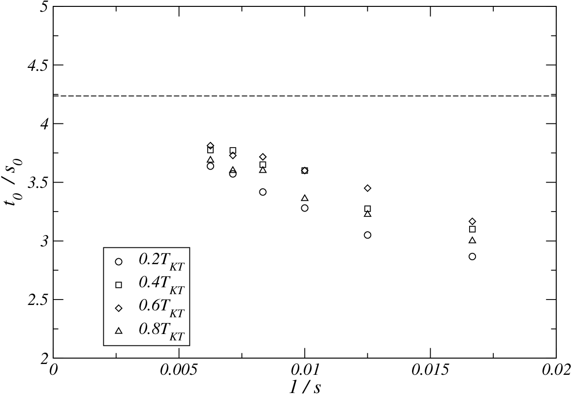
The prefactor corresponds to the quasi-equilibrium regime while the scaling function encodes the aging behavior of the correlation function. According to the aging hypothesis, the relevant scaling variable is where the characteristic length of domains is expected to grow as , i.e. algebraically (infinite relaxation time) with a logarithmic correction due to the pinning of the domain walls by the free vortices present in the paramagnetic phase [30]. In the case of the XY model, the dynamical exponent is . To test eq. (11), we have performed Monte Carlo simulations for a lattice size with a final time . The data have been averaged over 5000 histories. The data are noisier than in the low-temperature and it is not possible to obtain a more accurate estimate of from the quasi-equilibrium regime. On figure 8, the scaling function is plotted versus . The different curves correspond to waiting times and . The collapse of the different curves has been obtained using . We are left with an algebraic decay that confirms the scaling hypothesis (11). A close inspection of the effective exponents for the different waiting times reveals an evolution with . On the inset of fig 8 the effective exponents calculated using a power-law fit in the window are plotted versus . The different curves correspond to the different waiting times . Again, the large fluctuations for the leftmost points (larger values of ) occur at the same value of , independently of the waiting time . We thus interpret them as due to an under-sampling of the correlation causing systematic deviations of the effective exponents when the number of points entering into the interpolation becomes small. As a consequence, we have to consider the plateaus. An evolution with of the effective exponents on these plateaus is clearly perceptible. The exponents are plotted on figure 8. The extrapolation for leads to and thus, defining the autocorrelation exponent as [32] , we obtain . This value is slightly larger than the one obtained in the short-time regime from the initial-slip exponent () [19]. Note that short-time dynamics is equivalent to our analysis with [33] and is thus unable to give a correct estimate if the effective exponent evolves strongly with the waiting time . Both our estimate of and that obtained by Short-Time Dynamics are incompatible with the autocorrelation exponent of the XY model: [19], [22] or [34].


Again the response is too noisy to investigate its asymptotic scaling behavior but, using smaller lattice sizes and final times, it is still possible to improve significantly the statistics and estimate accurately the fluctuation-dissipation ratio. We have used a lattice size with time running up to . This allowed us to average the data over histories. On figure 9, the FDR is plotted with respect to . A good collapse of the data for different waiting times is observed. This collapse is not as good if logarithmic corrections are omitted. The asymptotic value of the FDR is estimated to be . In contradistinction to the algebraic decay of the spin-spin correlation function, does not present any evolution with the waiting time . For comparison, we have performed a similar simulation for the pure XY model. The asymptotic FDR is estimated to be for the XY model, i.e. very different from our value for the FFXY.

3 Aging of the chirality
We have also investigated the dynamics of the chirality, denoted in the following. For each plaquette, the local chirality is defined as
| (12) |
where the sum extends over the four bonds forming the plaquette. Chirality is expected to behave as antiferromagnetically-coupled Ising spins but a controversy exists regarding the belonging of the associated transition to the Ising universality class. In the following, we will compare two-time chirality-chirality correlation functions and the FDR associated to the response to a field coupled to the chirality with those of the Ising model.

The system is initially prepared in the paramagnetic phase and then quench at the critical temperature. We have considered two different estimates of the critical temperature: [17, 18] and [12]. We have computed the two-time chirality-chirality correlation function
| (13) |
for a lattice size up to the final time . Data have been averaged over 5000 histories. During a quench at the critical temperature, autocorrelation functions are expected to behave as where the first term corresponds to the quasi-equilibrium regime characterized by a critical exponent and the second one is the aging part depending only on the ratio . In the FFXY, we assume that the existence of free topological defects in the high-temperature induces logarithmic corrections in the growth law. Thus the correlation length for the chirality-chirality correlations is expected to grow as , i.e. in the same way as for the spin-spin correlation functions. As a consequence, we expect the scaling behavior
| (14) |
This behavior of the chirality-chirality correlation function is observed numerically
only with the estimate of the critical temperature. Figure 10
shows the collapse of the scaling function
versus for different waiting times. This collapse is clearly destroyed
when is chosen smaller than or larger than . This leads us to
, compatible with the Ising value .
We note that removing the logarithmic corrections does not affect significantly the
quality of the collapse. For the second and most accurate estimate of the critical
temperature , no collapse of the scaling function is obtained
for any positive value of (only a slightly negative value would bring the data
to collapse). This shows that the system is not critical in the quasi-equilibrium
regime but already in the low-temperature phase. In the following, we will consider
only the estimate of the critical temperature.
As shown on figure 10, the aging part of the chirality-chirality
correlation function decays algebraically. To recover the usual form in the asymptotic regime, the scaling function
needs to decay as . In the inset of figure 10
is plotted the effective exponent computed by a power-law interpolation in
the interval where runs from to . This effective exponent is
plotted with respect to for the different waiting times .
The exponent is recovered in the limit , i.e. at the left
side of the graph. Of course, in this region the number of points entering in the
interpolation is small and thus the accuracy of the effective exponent decreases.
Moreover, the data have been produced by a slow dynamics and are thus correlated. The
smooth variations at the left are really fluctuations and not any physical effect. From
this plot, we estimate , i.e. incompatible with the Ising value
(dashed line on the graph). Even though the curve of the
effective exponent for the largest waiting time is above the others, this cannot be
interpreted as an evolution of the exponents with . Indeed, the sequence of
curves is not ordered according to the waiting times. Our conclusion
is remarkably different from that drawn for the Ising-XY model in the low-temperature phase
for which an estimate compatible with that of the pure Ising
model was measured already for a relatively small final time [31].
For completeness, we should note that when we remove the logarithmic corrections,
the effective exponent is smaller, but still
incompatible with the Ising value. However, we believe that logarithmic corrections
are necessary as we will see in the following when considering the scaling of
the fluctuation-dissipation ratio.
The fluctuation-dissipation theorem is also violated at the phase transition. A Zeeman Hamiltonian
| (15) |
that couples the chirality of each plaquette to an external field , allows for the definition of a response function
| (16) |
This quantity is evaluated numerically [29]. We can then compute the fluctuation-dissipation ratio . We used a lattice size with a final time . Data have been averaged over histories. The FDR is plotted on figure 11 with respect to (left) and (right). A better collapse is obtained with logarithmic corrections, showing that the dynamics of the domain walls between different antiferromagnetic orderings of the chirality is sensible to the vortices. The asymptotic value is estimated to (a compatible value would be obtained if logarithmic corrections would not be taken into account). This value is significantly different from the Ising value [35]. Again, no evolution of with the waiting time is observed.

Conclusions
We have given numerical evidences that the thermal excitations in the low-temperature phase are spin-waves whose dynamics is the same as in the XY model. The dynamical exponent is thus in the whole critical phase. The exponent that can be estimated from the spin-spin two-time autocorrelation function is compatible with the prediction of the spin-wave approximation and with estimates from static Monte Carlo simulations close to . The fluctuation-dissipation ratio displays divergences, like in the XY model, at some locations that tend toward the value predicted by the scaling theory. When initially prepared in the paramagnetic phase and then quenched at (resp. ), spins (resp. chiralities) age in the same way as an unfrustrated ferromagnet. Spin-spin autocorrelation function decays slightly faster () than in the XY model. The FDR takes asymptotically a very different value too. These results are consistent with the fact that our estimate of is greater than the XY value, even though at the boundary of the error bar. The chirality-chirality autocorrelation function decays algebraically at the critical point with an exponent incompatible with that of the Ising model. The evolution of the effective exponent with the waiting time was taken into account. The FDR is also fully incompatible with the Ising value. No evolution of these values with the waiting time is visible, in contradistinction to static Monte Carlo simulations for which a cross-over is clearly observed when increasing the lattice size [14, 12]. The coupling between angles and chiralities is probably still too strong in the range of parameters used in our simulations. This coupling is manifest in the fact that the FDR is affected by logarithmic corrections that may be interpreted as an influence of the topological defects causing the Kosterlitz-Thouless transition. Moreover, the fact that our estimate of for the chirality is relatively close to the value measured at the Kosterlitz-Thouless temperature for the angles may also be the result of a strong coupling. To reach the cross-over regime and eventually enter the true critical regime, the correlation length should be allowed to reach much larger values. This requires of course larger lattice sizes but also larger times since . The computational effort scales with the lattice size as . It is therefore identical to static Monte simulations since the number of Monte Carlo steps needs to be increased when the lattice size increases and only local updates are possible for the FFXY. However, it seems that the amplitude is playing against us!
References
References
- [1] S. Teitel, C. Jayaprakash (1983) Phys. Rev. Lett. 51, 1999
- [2] J.M. Kosterlitz, D.J. Thouless (1973) J. Phys. C 6 1181 ; (1974) J. Phys. C 7 1046
- [3] S. Teitel, C. Jayaprakash (1983) Phys. Rev. B 27, 598
- [4] D. Loison, P. Simon (2000) Phys. Rev. B 61, 6114
- [5] M.Y. Choi, S. Doniach (1985) Phys. Rev. B 31 4516
- [6] Y.M.M. Knops, B. Nienhuis, H.J.F. Knops, H.W.J. Blöte (1994) Phys. Rev. B 50, 1061
- [7] J. Villain (1977) J. Phys. C 10 1717 ; (1977) J. Phys. C 10 4793
- [8] E. Fradkin, B. Huberman, S.H. Shenker (1978) Phys. Rev. B 18 4789
- [9] Z. Nussinov (2001) arXiv: cond-mat/0107339
- [10] S. E. Korshunov (2002) Phys. Rev. Lett. 88, 167007, arXiv: cond-mat/0106151
- [11] P. Olsson, S. Teitel (2005) Phys. Rev. B 71, 104423, arXiv: cond-mat/0304593
- [12] M. Hasenbusch, A. Pelissetto, E. Vicari (2005) J. Stat. Mech. 0512 P002, arXiv: cond-mat/0509682
- [13] P. Olsson (1995) Phys. Rev. Lett. 75, 2758, arXiv: cond-mat/9506082 ; P. Olsson (1997) Phys. Rev. B 55, 3585, arXiv: cond-mat/9609181
- [14] J.D. Noh, H. Rieger, M. Enderle, K. Knorr (2002) Phys. Rev. E 66, 026111
- [15] M. Hasenbusch, A. Pelissetto, E. Vicari (2006) J. Phys. Conf. Ser. 42 124, arXiv: cond-mat/0509511
- [16] H.J. Luo, B. Zheng (1997) Mod. Phys. Lett. B 11, 615, arXiv: cond-mat/9812147
- [17] H.J. Luo, L. Schuelke, B. Zheng (1998) Phys. Rev. E, 57 1327, arXiv: cond-mat/9705222
- [18] H.J. Luo, L. Schuelke, B. Zheng (1998) Phys. Rev. Lett. 81 (1998) 180, arXiv: cond-mat/9801253
- [19] H.J. Luo, M. Schulz, L. Schuelke, S. Trimper, B. Zheng (1998) Phys. Lett. A 250 383, arXiv: cond-mat/9812124
- [20] S.J. Lee, J.R. Lee, B. Kim (1995) Phys. Rev. E 51, R4
- [21] G.S. Jeon, S.J. Lee, M.Y. Choi (2003) Phys. Rev. B 67, 014501
- [22] B. Zheng, F. Ren, and H. Ren (2003) Phys. Rev. E 68, 046120
- [23] R.J. Glauber (1963) J. Math. Phys 4, 294
- [24] A.D. Rutenberg, A.J. Bray (1995), Phys. Rev. E 51, R1641
- [25] L.F. Cugliandolo and J. Kurchan, Phys. Rev. Lett. 71, 173 (1993) ; L.F. Cugliandolo and J. Kurchan, J. Phys. A: Math. Gen. 27, 5749 (1994)
- [26] S. Abriet, D. Karevski (2004), Eur. Phys. J. B 37, 47, arXiv: cond-mat/0309342
- [27] L. Berthier, P.C.W. Holdsworth, and M. Sellitto (2001) J. Phys. A 34, 1805
- [28] S. Abriet (2004), Ph.D. thesis (unpublished)
- [29] C. Chatelain (2003) J. Phys. A: Math. Gen. 36, 10739, arXiv: cond-mat/0303545
- [30] A.J. Bray, A.J. Briant and D.K. Jervis (2000) Phys. Rev. Lett. 84, 1503
- [31] J.R. Lee, S.J. Lee, B. Kim, I. Chang (1996) Phys. Rev. E 54, 3257
- [32] D. Huse, Phys. Rev. B 40, 304 (1989)
- [33] T. Tomê, M.J. de Oliveira (1998) Phys. Rev. E 58, 4242
- [34] X. W. Lei and B. Zheng (2007) Phys. Rev. E 75, 040104(R)
- [35] C. Chatelain (2004) J. Stat. Mech.: Theor. Exp. P06006, arXiv: cond-mat/0404017