IPPP/09/24
DCPT/09/48
August 24, 2026
Soft physics at the LHC11
1
Topical Review to be published in J.Phys.G, based on two lectures by Misha Ryskin at the St. Petersburg Winter School, Gatchina, February 2009
M.G. Ryskina,b, A.D. Martina, V.A. Khozea,b and A.G. Shuvaevb
a Institute for Particle Physics Phenomenology, University of Durham, Durham, DH1 3LE
b Petersburg Nuclear Physics Institute, Gatchina, St. Petersburg, 188300, Russia
We recall the main features of the Regge approach used to understand soft interactions at LHC and higher energies. Unitarity tames the power growth of the elastic proton-proton scattering amplitude with energy, and leads to the migration of the secondary particles produced in high-energy proton-proton collisions to larger transverse momenta. We discuss, in qualitative terms, the role of processes containing large rapidity gaps (LRG), and the probability that the gaps survive population by secondaries produced in additional soft interactions. We explain how the Regge diagram corresponding to a LRG event simultaneously describes events with different (single, double, etc.) particle density in the same rapidity interval. We show that the role of these, enhanced, multi-Pomeron diagrams can be studied by measuring multiplicity fluctuations and long-range rapidity correlations between secondaries produced at the Tevatron and the LHC. Finally, we make a list of the characteristic features of the multi-Pomeron description of soft interactions that may be observed at the high energies accessible at the Tevatron and the LHC.
1 Introduction
“Soft” physics is manifest in various places in different guises. The interest in soft interactions at very high energies is stimulated, theoretically, by the fact that the observed hadronic cross sections are growing with energy and, experimentally, by the advent of the LHC.
At the LHC energy we have to allow for unitarity effects, which are necessary to provide the consistency of the strong interaction. In fact, when we face a cross section which grows as a power of the energy, there are two possible ways to restore unitarity.
First, we may introduce a new particle (sufficiently heavy to have not been observed yet) which cancels the growth of the cross section at energies larger than the mass of the particle (for example, Higgs boson, super-partners, etc.). After this, we deal with a weak interaction, where the main contribution comes from one, or a few, simple diagrams. More complicated Feynman graphs just describe corrections to the lowest-order amplitude.
Another possibility is to consider a strong interaction. Here, from the beginning, we start with a Hermitian Lagrangian, which should already account for unitarity. When the Born amplitude (or an amplitude obtained via the summation of some group of diagrams) becomes too large and the interaction becomes strong, then new more complicated diagrams must enter the game. It is the contribution due to these new graphs which tames the growth of cross section such that the final result satisfies unitarity.
In the case of QCD, where the BFKL amplitude () grows as a non-integer power () of energy, , we expect to observe the second scenario22 2 It looks impossible to cancel the non-integer power of by introducing a new particle.. Therefore it is important to observe, and to study, the role of more complicated diagrams (arising from multiple interactions) at LHC energies, and to trace how the theory restores the unitarity of the strong interaction. That is, from a theoretical viewpoint, it is of great interest to observe experimentally how unitarity tames the growth of high-energy hadronic amplitudes, leading to saturation both in the transverse momenta and in the impact parameter distributions of the produced particles. In other words, unitarity replaces the growth of the amplitude by the growth of configuration space occupied by the particles, both in and in .
Here, we do not present new results but attempt to recall, using modern language, the ideas and understanding of high-energy soft interactions which originated some 40 or more years ago. The discussion may be divided into three main topics: (i) elastic scattering and the total cross section, (ii) the cross sections of processes with gaps in rapidity (including high-mass diffractive dissociation), and, (iii) the saturation of particle densities in transverse momenta .
Soft high-energy interactions are clearly important at the LHC. Moreover, they can complicate our ability to observe new physics. For example, topic (iii) is relevant to the search for new physics, since particles with a rather large from the underlying inclusive event will affect the jet searching algorithm, as is already the case for jets at HERA and the Tevatron. On the other hand, the evaluation of the cross section for an exclusive process, such as , requires knowledge of the gap survival probability , which is the subject of topic (ii), see, for example, [1, 2, 3, 4].
Here, we focus on the qualitative features of high energy soft interactions. These features are quite general. With the advent of the LHC, it is timely to gather them together and to emphasize the underlying physics.
2 Total and elastic cross sections
The behaviour of scattering amplitudes in the high energy, , small momentum-transfer squared, , domain is well described by Regge theory; that is, by the singularities of amplitudes in the complex angular momentum, , plane, see, for example, [5, 6]. For instance, the measured amplitude behaves as
| (1) |
where the -trajectory, (with in ), passes through the spin-1 -meson resonance in the ‘crossed’ -channel ; that is, .
On the other hand, total cross sections are observed to grow slowly with energy and are associated with the exchange of a trajectory with vacuum quantum numbers. The simplest possibility is to assume that at high energy these cross sections, such as the total cross section , are driven by an isolated pole at , which gives an () elastic amplitude
| (2) |
and, via the optical theorem of Fig. 1, a total cross section
| (3) |
The pole with the largest intercept, originally with since high energy total cross sections were thought to have constant asymptotic behaviour, was called the Pomeron33 3 A discussion of the history of the Pomeron is given in [6].. Here we are interested in Tevatron and higher energies which are sufficiently large to be able to neglect the contributions of all secondary trajectories (which all have intercepts ).

A popular parametrization of elastic -scattering amplitude by Donnachie-Landshoff (DL) is the Regge form [7]
| (4) |
where the signature factor gives the complex phase, is the electromagnetic form factor of the proton, and the effective soft Pomeron trajectory
| (5) |
where is in GeV2. The intercept just above 1 reproduces the observed slow growth of the total hadron-hadron cross sections at high energies. Indeed, the effective Pomeron pole amplitude, (4), gives a good description of the total and elastic differential cross section data up to Tevatron energies. However, this simple parametrization is expected to become increasingly deficient at higher energies. Unitarity is an easy way to see this.
To discuss unitarity effects it is convenient to work in impact parameter, , space, since at high energy the position of the particle in is practically frozen. Thus the value of determines the orbital momentum of the incoming proton, ; that is, fixed corresponds to a particular partial wave . In space the elastic unitarity equation44 4 The amplitude is normalised to .
| (6) |
limits the value of . However, this limit corresponds to a pure elastic interaction with phase of elastic amplitude,
| (7) |
equal to . Normally at high energies the inelastic contribution dominates, leading to a large inelasticity; that is, to a large imaginary part, . In this so-called ‘black disk’ limit55 5 In general, an amplitude with is not forbidden. The corresponding model, so-called -matrix unitarisation, was discussed in [8]. However, such a model which asymptotically leads to a pure elastic interaction, without any particle production, does not look probable., we have . Recall that, if we were to neglect the small contribution from the real part, then Im can be measured directly from experiment as the Fourier transform
| (8) |
where , is a Bessel function and .
Note that the DL amplitude crosses the black disk limit between the Tevatron and LHC energies, see Fig. 2. Thus we expect that at the LHC the cross section will be less than that given by the DL parametrization, while the slope of elastic cross section, , should be larger. The partons occurring in the proton wave function will be pushed away from the centre to the periphery. This suppression of the amplitude at low values of automatically increases the elastic slope , since where is the interaction radius.
For this reason the value of GeV-2 in (5) should not be considered as the slope of the bare Pomeron trajectory. Part of this slope is generated by the stronger absorptive corrections at smaller . Indeed, the shrinkage of the diffractive cone observed in deep-inelastic scattering at HERA (say, in -meson or in diffractive production) is smaller than that observed in -scattering.

Actually to satisfy elastic unitarity it is sufficient to consider an eikonal model which sums up the exchanges of any number of Pomerons between the incoming protons. The model gives a result analogous to (7)
| (9) |
where, up to a normalization factor, the opacity plays the role of the scattering phase . In the eikonal model, (9), it is the opacity which is now described (or parametrised) by Pomeron exchange, rather than the final amplitude . The situation is sketched symbolically in Fig. 3(a). However this is not the whole story. The eikonal model does not include events with Large Rapidity Gaps (LRG), arising from the dissociation of one or both of the protons into high-mass systems, which are observed experimentally. We speak of single or double high-mass diffractive dissociation. We introduce high-mass dissociation in the next Section and give detailed discussion of these LRG events in Section 5.
Before we do this, let us recall that the interaction radius (i.e. the elastic slope) expected at the LHC will already exceed 1 fm – the distance where confinement may enter the game. Thus it is possible that confinement will stop the growth of the radius; that is, the growth of . Another interesting possibility, proposed by V.V.Anisovich [10], is that the partons (the gluons and quarks) in the proton will start to form a few colourless clusters (like the nucleons in nucleus), rather than the normal homogeneous distribution. This may lead to a rich diffractive dip structure in the differential elastic cross section . It is an additional argument to study experimentally the behaviour of the elastic cross section at the LHC66 6 Reviews of the predictions for the total cross section, and the elastic scattering cross section over an extended interval, can be found in [11]..
3 Diffractive dissociation
So much for elastic scattering, which we may call elastic diffraction. Now we turn to inelastic diffraction, which is a consequence of the internal structure of the protons. Besides the pure elastic two-particle intermediate states shown in Fig. 3(a), there is the possibility of proton excitation, , shown in the small sketch in Fig. 3(b). At high energies, when the lifetime of the fluctuations of the fast proton is large, , the corresponding Fock states can be considered to be ‘frozen’. Each constituent of the proton can undergo scattering and thus destroy the coherence of the fluctuations. As a consequence, the outgoing superposition of states will be different from the incident particle, so we will have inelastic, as well as elastic, diffraction.

To discuss inelastic diffraction, it is convenient to follow Good and Walker [12], and to introduce states which diagonalize the matrix. These, so-called diffractive, eigenstates only undergo ‘elastic’ scattering. To account for the internal structure of the proton we, therefore, have to enlarge the set of intermediate states, from just the single elastic channel, and to introduce a multi-channel eikonal. The situation is pictured in Fig. 3(b).
What about proton dissociation into high-mass systems? At first sight, it appears that we may account for it by simply enlarging the number of diffractive eigenstates . Even if this were practical, we would still face the problem of double counting when partons originating from the dissociation of the beam and the ‘target’ protons overlap in rapidities. Instead, high-mass dissociation is described in terms of so-called “enhanced” multi-Pomeron diagrams. The first, and simplest, is the triple-Pomeron diagram, shown in Fig. 1 and again in Fig. 3(c). In fact, high-mass dissociation is much larger than low-mass dissociation at very high energy, and it will play a central role in our discussion of soft interactions. For simplicity, therefore, we do not discuss low-mass dissociation further, but consider that it can be easily allowed for in terms of a multi-channel eikonal. So, from now on we should regard as an effective opacity embodying low-mass dissociation.
Why does high-mass dissociation become so important at high collider energies? A simplified way to see this is to note that the cross section for dissociation of a proton into a high-mass () system has the approximate form77 7 Here, for simplicity, we assume an essentially flat energy dependence, with . The final equality in (10) can be deduced by taking the ratio of the couplings indicated in the Regge expressions in Fig. 1.
| (10) |
with , where is the triple-Pomeron coupling and is the coupling of the Pomeron to the proton, see Fig. 1. The ln ‘rapidity’ factor comes from the integration . Note that here we have used and , see Fig 1. Eq. (10) is grossly oversimplified. For one thing, the dissociation cross section is subject to even greater absorptive (that is, multi-Pomeron) corrections than the elastic cross section. When these are taken into account it is found from analyses of the available high-energy data that
| (11) |
see, for example, [9]. The important point is that the relative size of the and cross sections is governed, not simply by the parameter , but rather by . For each fixed rapidity interval the probability of high-mass dissociation is relatively small, but the cumulative effect in the complete interaction amplitude is enhanced by the large phase available in rapidity at high collider energies.
4 The structure of the Pomeron
In the Regge approach, we have seen that high-energy soft interactions are driven by Pomeron exchange, together with its absorptive (multi-Pomeron) corrections. We may call this the “soft” Pomeron. Note that the -channel asymptotic behaviour arising from -channel Pomeron exchange corresponds to an interaction radius which grows with energy, . The Pomeron must also describe multiparticle interactions. The sum of ladder diagrams of the type of Fig. 4(a) is the simplest multiparticle structure which reproduces the power-like behaviour of the Pomeron pole. Before the advent of QCD, ladder diagrams composed of -channel mesons (dominantly spinless pion exchange88 8 Pion-exchange was considered to be the dominant mechanism due to the proximity of the pion pole, at , to the -channel physical domain ,, due to the smallness of the pion mass.) were summed, and it proved difficult to generate an intercept .
Shortly after the discovery of QCD it was noticed [13] that (colourless) two-gluon exchange has the properties of Pomeron exchange: vacuum quantum numbers, even signature and a singularity at . Due to the polarisation vectors of the spin-one particle (the gluon), the numerator of the propagator contains the tensor such that the 4-momenta of the incoming fast protons occur in the form . Therefore the gluon-exchange amplitude contains an extra power of as compared with spinless particle exchange.
Later, by applying the Regge approach to gluons, rather than to hadrons, it was possible, if the gluon transverse momenta were sufficiently large, to describe high energy (low ) interactions in terms of perturbative QCD. Then, on summing the leading contributions, where the smallness of the QCD coupling is compensated by large values of ln, we build up the “hard” Pomeron. Below, we briefly trace this history and then apply these ideas to gain insight into high-energy soft interactions.
4.1 Ladder structure of the Pomeron pole before QCD
In terms of Regge theory, the high-energy amplitude is described by the exchange of a Pomeron (or a few Pomerons). As mentioned above, from a quantum field theory viewpoint, the Pomeron may be regarded as the sum of ladder-type diagrams, Fig. 4(a). In other words, it corresponds to a sum of completely inelastic processes; that is, to the last term in the unitarity equation (6). Now let us ‘cut’ the Pomeron; see Section 5.2 for further discussion. That is, we treat the graph of Fig. 4(a), not as a diagram for the amplitude, but rather as the diagram for the cross section
| (12) |
see Fig. 4(b). Then, we get the inelastic production of particles homogeneously distributed in the available rapidity, , interval.
In the original ‘soft’ Regge approach it was assumed that the transverse momenta of these secondaries were limited99 9 Nowadays, with QCD, as mentioned above and discussed below, the Pomeron is described by a ladder built of the gluons. As a result, due to the dimensionless QCD coupling, there is no parameter to limit the value of , and BFKL equation predicts the ‘diffusion’ of the gluons in space [14].. The original idea, proposed by Amati, Fubini and Stanghellini in 1962 [15], was to explain a large high-energy cross section, which did not decrease with energy, as a sequence of interactions in which the energy of a pair of adjacent particles (pions) is relatively small and lies in the resonance region where the interaction is strong. The integration corresponding to each cell of such a ladder is over the rapidity and the transverse momentum , see Fig. 4(a). If we denote the momentum transferred through the whole ladder by , then the contribution from a particular cell is where
| (13) |
and is the coupling. The integration over the rapidities gives
| (14) |
where the total rapidity spanned by the ladder , and reflects the identity of the cells or, equivalently, the ordering of the rapidities .

A convenient alternative way to obtain this result is to consider the evolution equation in rapidity
| (15) |
In such a form plays a role similar to a DGLAP splitting function.
Note that the value of the ‘effective spin’ depends on the momentum transfer through the ladder, . The slope of the Pomeron trajectory at is controlled by the mean value of the transverse momenta or, in the case of (13), by the mass of the -channel particle.
However, with this procedure it turns out to be practically impossible to obtain a large intercept whilst keeping the -channel exchanges to have masses GeV. The corresponding couplings are too small. On the other hand, if we include heavier states, then we go to larger ; that is to small distances where it looks reasonable to work in terms of perturbative QCD.
4.2 Ladder structure of the Pomeron pole after QCD
With QCD, the Pomeron, at least at small distances, is described by the ladder of Fig. 4(a) built of gluons, rather than of spinless particles; with the coupling in (13) replaced by the QCD coupling . The integral over now has a more complicated structure. It is convenient to consider the recursion relation between the amplitudes with and cells
| (16) |
where we keep just the leading ln term in the integration. Note that now we have to account for the dependence of the amplitude on the transverse momenta, , of the -channel gluons. The recursion relation may be rewritten in differential form, as the BFKL evolution equation [16]
| (17) |
so that , where
| (18) |
where is the leading eigenvalue calculated using equation (20) below. Since we now have spin-one gluons in the ladder, the intercept already in the limit .
In fact, if just the leading ln contributions are summed then, explicitly, 4ln2, where [16]. However, the next-to-leading logarithm (NLL) contributions are numerically rather large. It was found [17] that, accounting these corrections, . For the relevant, not too small, values of , a resummation is necessary. Since the NLL contribution is mainly of kinematic origin, it is possible, and looks reasonable, to resum all the major higher-order corrections. This leads to [18] in a wide region of .
For simplicity, we consider just the forward amplitude1010 10 For non-zero the kernel is a bit more complicated, but qualitatively similar in form. with . Then the elastic forward amplitude is
| (19) |
and, at LO, the BFKL kernel acts as
| (20) |
Since in QCD we deal with a dimensionless coupling and a massless gluon, the mean value of in each cell is determined by the value of transverse momentum in the previous cell. This is an important property of the BFKL equation – that is, the so-called diffusion in . The value of in the current cell may differ from that in the previous cell by some quantity . In other words, at each step of evolution, not only the impact parameter can be changed by , but also the value of can be changed by .
4.3 The transition from the ‘hard’ to the ‘soft’ Pomeron
There are phenomenological hints that at large distances the “soft” Pomeron should have qualitatively similar structure as the “hard” (QCD) Pomeron. Indeed, first, no irregularity is observed in the HERA data in the transition region, , between the ‘soft’ and ‘hard’ interaction domains; the data are smooth throughout this region. Second, a small slope of the Pomeron trajectory, is obtained in global analyses of all available soft high-energy data, after accounting for absorptive corrections and secondary Reggeon contributions. This indicates that the typical values of inside the Pomeron amplitude are relatively large (). Finally, recent ‘soft’ model data analyses [9, 19, 20] which account for the enhanced absorptive effects find an intercept of the initial, bare Pomeron close to the intercept of the BFKL Pomeron after the NLL corrections are resummed [18]. Thus it looks reasonable to assume that in the soft domain we deal with the same perturbative QCD Pomeron; at least, there is a smooth transition from the soft to the hard Pomeron.
In summary, the bare hard Pomeron, with a trajectory with intercept and small slope , is subject to increasing absorptive effects as we go to smaller which allow it to smoothly match on to the attributes of the soft Pomeron. In the limited energy interval up to the Tevatron energy, some of these attributes (specifically those related to the elastic amplitude) can be mimicked or approximated by an effective Pomeron pole with trajectory intercept and slope .
5 Events with Large Rapidity Gaps
For further discussion, we write the BFKL evolution equation (17) in the oversimplified form
| (21) |
where acts as the splitting function. This evolution equation is the analogue of (15), but, now, the possibility of multiparticle production leads to an additional power growth of the amplitude, , in comparison with the Born amplitude, . In other words, the evolution (21) describes the development of the parton cascade from the ‘beam’ proton to the ‘target’ proton, and the growth of the inelastic cross section reflects the power growth of the parton density in the cascade.
After one of the partons interacts with the target the coherency of the beam proton wave function is destroyed and a number of secondaries is produced. Note that in the ladder of Fig. 4(b) only one branch of the whole cascade is shown, which finally leads to a parton being absorbed by the target. The number of secondaries produced is equal to the number of steps (partons) in this particular branch, shown in Fig. 4(b). According to (21), where plays the role of the particle density per unit of rapidity, we have . On the other hand, each of the partons continue to develop its own cascade. One example is shown in Fig. 4(b), where parton develops its own branch. However, the branches which were not affected by the target conserve their coherence, and in the final state appear as a single parton. Thus we get the power growth of the amplitude, but only a logarithmic growth of the multiplicity . The studies of coherence phenomena in a partonic cascade were pioneered by V.N. Gribov in 1972, see [21].
5.1 Large Rapidity Gap contribution to the total cross section
The fact that the coherence of the wave function of the beam proton was destroyed after the interaction with the target, leads not only to inelastic high-multiplicity production, but via unitarity relation (6), also to elastic scattering. Elastic scattering is due to the absorption of an initial (coherent) component in some domain of the impact parameter plane, and originates from the remaining part of the initial wave function which conserves the coherence between the partons. That is, elastic scattering occurs as the ‘shadow’ of the inelastic interaction. If the inelastic contribution is represented by the single ladder of Fig. 4(b), then the elastic contribution may be drawn as a ‘cut’ between the two Pomerons of Fig. 4(c), see also Fig. 6.
So much for elastic scattering of the incoming proton. However, an intermediate parton in a ladder may be scattered elastically as well. A unitarity equation, analogous to (6), may, and should be, written for any intermediate parton. The elastic scattering of an intermediate parton can be represented by the diagram of Fig. 4(d). Here, both branches of the cascade which start to evolve from parton save their coherence. Therefore in the final state we will have a Large Rapidity Gap between the parton and the target. Such a process is called the diffractive dissociation of the beam proton into a high-mass state . It is described by the triple-Pomeron diagram of Fig. 4(e), in which one Pomeron is split into two Pomerons, see also Fig. 1. The probability of this splitting within a unit rapidity interval is relatively small. First, due to the small parton density , where arises from (21). Next, due to the parton-(target) proton cross section being smaller than the proton-proton cross section, since the incoming proton contains many partons. On the other hand, each intermediate parton in the ladder may generate a Pomeron splitting. Thus, the whole effect accumulated during the evolution (21) is enhanced by the parton multiplicity – in other words, by the size of available rapidity space , see also the discussion around equation (10). Therefore a triple-Pomeron diagram (like that in Fig. 4(e)) or diagrams with more complicated multi-Pomeron vertices (like those in Fig. 5(b)) are called enhanced diagrams.
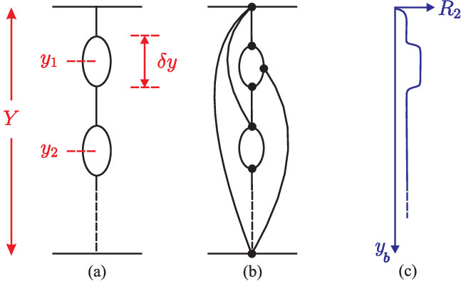
Already at the Tevatron, the cross section of the events with a LRG, that is of single- and double-diffractive dissociation of one or both protons (integrated over the mass of the final ‘diffracted states’), is comparable to the elastic cross section. If we were to take the contribution of the diagram of Fig. 4(e) literally and integrate over the rapidity of vertex , then, at sufficiently high energy, the cross section of events with a LRG would exceed the whole inelastic contribution described by a single Pomeron, that is the contribution of Fig. 4(b) (recall ).
The situation is even worse when we consider events containing a large number of LRG, arising, for example, from the multi-Pomeron diagram of Fig. 5(a). For simplicity, let us first account for gaps of limited size, say . We denote the probability to form such a gap as . Then, integrating over the central position of each gap, we obtain for the contribution
which grows as a power of . If we neglect the limit , and allow for the integration over the gap size , then the cross section increases faster than any power of , and clearly violates unitarity. This problem was discussed long ago in [22].
Two main scenarios were proposed to prevent such a growth and to restore unitarity. First, the so-called weak coupling scenario assumes that the triple-Pomeron vertex (and correspondingly the value of ) vanishes as [23]. Since the mean value of momentum transfer decreases as (the shrinkage of the diffractive cone) the decrease of compensates the increase of the available rapidity interval. However this hypothesis is not supported by experiment1111 11 Still the weak coupling possibility is not rejected completely and it will be important to study high-mass dissociation at the LHC in the low region to confirm this conclusion; see [24]..
In the favoured strong coupling scenario [25], the multi-gap cross section is suppressed by a small ‘gap survival probability’ which decreases with energy. In this case the Pomeron coupling as , while the small probability of LRG production is due to the large probability that the gaps are populated by secondaries produced in additional soft rescattering interactions between the protons (and also the intermediate partons).
In the simple eikonal model, (9), the probability, not to have an additional inelastic interaction which will populate the gap, is given by a factor . Recall that in the eikonal model . However, this factor accounts for the rescattering of the incoming protons only. Since, now, we have also rescattering between the intermediate partons we have to consider more complicated multi-Pomeron diagrams, like those shown in Fig.3(c).
5.2 Multi-Pomeron diagrams and the AGK cutting rules
We emphasize that each multi-Pomeron exchange diagram describes simultaneously a few different processes. We have already seen that the first ladder diagram gives, on the one hand, the elastic scattering amplitude, Fig. 4(a), while, on the other hand, it may be considered as the ‘cut’ diagram for the cross section for multiparticle production, Fig. 4(b). In the latter case cutting the Pomeron of Fig. 4(a), that is taking the discontinuity, disc=2Im, gives the contribution to multiparticle production, .

Now consider the two-Pomeron exchange diagram of Fig. 4(c). Strictly speaking, the diagram should be drawn more precisely, as has been done in Fig. 6. We have the possibility to cut both Pomerons simultaneously, 6(d), to cut only one Pomeron, 6(c), or to cut between the two Pomerons, 6(b). The sum of all cuts gives the total contribution of two-Pomeron exchange to the imaginary part of the elastic amplitude. This contribution is negative and describes the absorptive correction to the one-Pomeron amplitude. On the other hand, the elastic cross section corresponding to Fig. 6(b) is positive; as is the cross section of the events with a ‘doubled’ particle density, which we obtain by cutting both Pomerons as in Fig. 6(d). The only negative contribution is the absorptive correction to the events with a single particle density (i.e. the correction to single-Pomeron exchange). The famous AGK cutting rules [26] gives the relation between the different subprocesses originating from the same Reggeon diagram. For the respective cut diagrams of Fig. 6, the relation is
| (22) |
while the whole contribution to the elastic amplitude is .
Analogous relations hold for more complicated diagrams with many Pomerons. Note that, according to the AGK rules, the multi-Pomeron diagrams do not change the single particle inclusive cross section . Indeed, the particle density arising from diagram 6(d) is twice larger than that from 6(c), and these two contributions cancel each other. The same is true for more complicated multi-Pomeron diagrams.
If we start with the eikonal model, then the sum of all the multi-Pomeron exchange diagrams gives the total probability of the interaction at fixed ,
| (23) |
where is given by one-Pomeron exchange and
| (24) |
Here, is the probability of the elastic interaction; and is the probability to produce a particle density times larger than that arising from one-Pomeron exchange, that is the probability to cut Pomerons in the whole amplitude. It is easy to see that
| (25) |
is the whole inelastic contribution at a fixed . The penultimate expression for represents the whole probability, 1, minus the probability to have no inelastic interaction, whereas in the previous expression for each term represents the probability of inelastic interactions (where accounts for the identity of the interactions) multiplied by which guarantees that there are no further inelastic interactions. The multi-Pomeron exchange structure of processes of (23)-(25) is sketched in Fig. 7.

Similar rules, with the same combinatorics, are valid in the presence of enhanced screening. At each multi-Pomeron vertex, we can cut one or more Pomerons, or cut between the Pomerons placing the uncut Pomerons either to the left or to the right of the cut. For illustration, we discuss the contributions arising from cutting a triple-Pomeron diagram which is screened by a single eikonal Pomeron, as shown in Fig. 8(a). The Pomeron ladders corresponding to this diagram, Fig. 8(b), can be cut in 8 different ways. First, we have the elastic cut between all the ladders. Next, the cut of the eikonal Pomeron ladder gives the usual single-Pomeron multiplicity. Then, we have three possibilities to cut the triple-Pomeron graph; one with single multiplicity in the whole rapidity interval, one with a gap in the upper part, one with double multiplicity in the upper part. Finally, we have the same three, but now simultaneously cutting the eikonal Pomeron. Thus, the different cuts, which lead to 8 different process, give the particle multiplicities as a function of rapidity that are sketched in Fig. 8(c). The AGK cutting rules may be used to determine the relative probabilities of these processes; the result is given below the multiplicity plots. For the example of Fig. 8 we have to use relation (22) twice. For instance, the probability comes from , whereas comes from ( corresponds to the cut of the triple-Pomeron diagram without cutting the single Pomeron; note that in (22) , where the two terms correspond to cutting one or the other Pomeron in Fig.6).

Moreover, AGK rules show that, in general, these factors do not depend on exactly how the multi-Pomeron vertices are cut. To be specific, the probability of a particular subprocess is given just by the combinatorial factors to choose cut Pomerons from Pomerons of the original amplitude. A factor 2 comes from disc=2Im of each cut Pomeron, and another factor 2 comes from the possibility to place any uncut Pomeron to the right or left of the cut.
5.3 Long-range rapidity correlations
Note that the eikonal model (9) predicts a long-range correlation between the secondaries produced in different rapidity intervals. Indeed, we have possibility to cut any number of Pomerons. Cutting Pomerons we get an event with multiplicity times larger than that generated by one Pomeron. The probability to observe a particle from a diagram where Pomerons are cut is times larger than that from the diagram with only one cut Pomeron. The observation of a particle at rapidity , say, has the effect of enlarging the relative contribution of diagrams with a larger number of cut Pomerons. For this reason the probability to observe another particle at quite a different rapidity becomes larger as well. This can be observed experimentally via the ratio of inclusive cross sections
| (26) |
where is the particle density.
Without multi-Pomeron effects the value of exceeds zero only when the two particles are close to each other, that is when the separation is not large. Such short-range correlations arise from resonance or jet production. However, multi-Pomeron exchange leads to a long-range correlation, , even for a large rapidity difference between the particles, . In fact, such a long-range correlation, with for , has even already been observed in the old CERN-ISR data [27].
In the eikonal case, the value of may be calculated explicitly from the Poisson distribution of given in (24). At fixed it gives
| (27) |
For a low optical density the correlation arises mainly from the two-Pomeron exchange diagram, and increases as . At very large , the Poisson distribution becomes narrow in the number of cut Pomerons, and decreases as . The maximum value is for .
It would be informative to study the Pomeron loop structure by observing long-range correlations at the LHC energy. In the pure eikonal case, the correlation should be the same throughout the whole available rapidity interval (except, of course, near the edges of rapidity interval, where multiparticle production is affected by energy conservation constraints). When we have enhanced diagrams, that is Pomeron loops which produce LRG which occupy only a part of the rapidity space, the corresponding correlation takes place only within this interval. Thus the existence of Pomeron loops may be revealed both as LRG events (from the cut with zero multiplicity inside the interval), and as long-range correlations in the intervals (from the cuts generating large multiplicities of secondaries). The ‘range’ of the correlation reflects the size of the Pomeron loop in rapidity space. An example of this behaviour of is shown in Fig. 5(c)
5.4 The decreasing cross section
Note that the simplest scenario to restore the unitarity at very high energies is not yet completely rejected. We mean the possibility that asymptotically the Pomeron intercept becomes less than 1, , and at very high energies the total cross section starts to decrease with energy. Such a behaviour is expected in a theory with only the triple-Pomeron coupling, and which neglects the more complicated multi-Pomeron vertices, such as the Pomeron coupling and so on [28].
Recall that the two-Pomeron loop gives a positive probability for LRG production but its contribution to the amplitude is negative, see Fig. 6. If we now sum up the diagrams with many two-Pomeron loop insertions (Fig. 5(a)) then we ‘renormalise’ the Pomeron propagator. In this way we obtain the ‘dressed’ propagator in terms of a Schwinger-Dyson equation. The intercept of the final ‘dressed’ propagator is . With increasing energy, the available rapidity interval increases, with the result that the loop renormalisation grows and hence the effective intercept decreases. Asymptotically, the Schwinger-Dyson equation gives
| (28) |
where is the triple-Pomeron coupling. The loop contribution, , is calculated using the dressed Pomeron propagator, and the factor comes from the integral over the loop size .1212 12 Strictly speaking, there should also be a Schwinger-Dyson equation giving the dressed triple-Pomeron coupling. However, in this oversimplified estimate, we have truncated the system of Schwinger-Dyson equations at the first step.
For the reasonable values and , the naive estimate based on (28) gives . That is . This means that up to a rather large energy () the total cross section will grow, but after this, that is just in the LHC region, it will start to decrease. For multiparticle production, such a regime will reveal itself as long-range rapidity fluctuations of the multiplicity arising from two-Pomeron loops which may produce either LRG or a double multiplicity of secondaries in the rapidity domain occupied by the loop.
6 Saturation of the distribution
Let us return to the simplified eikonal model (9), written for the partons in the incoming protons. We may ask the question - “what happens to an incoming fast quark?” On the one hand, the factor describes its absorption. After the inelastic collision the incoming quark disappears from the initial wave function. On the other hand, the quark cannot just disappear1313 13 For the gluon the situation is more complicated. Some of gluons can disappear via fusion, .. It has baryon charge, etc. Disappearance from the incoming beam (wave function) actually means migration – after the collision the momentum of quark is changed. In the leading logarithmic approximation, the quark mainly changes its transverse momentum. Each new Pomeron-quark coupling may be considered as a new elastic scattering and it is known that after scatterings the mean transverse momentum squared, , increases times.
Thus, when we say that unitarity stops the growth of the parton density via an increase of the absorptive correction, actually we mean that the extra partons produced by the cascade are pushed out of the previous domain in configuration space into a region of larger and . Accounting for the enhanced diagrams we get the same phenomena, not only for the incoming fast partons (as in the eikonal model), but for any intermediate partons as well. Thus finally we expect that the particle density will reach saturation at low , but will continue to grow with energy at larger . Therefore, at higher energies a larger number of minijets with larger will be produced.
Due to saturation in the low region at very high energies, the majority of partons will have rather large . We already know that the diffusion in takes place in the perturbative QCD domain [14], and to provide a smooth matching to the larger domain we need to include some elements of a similar diffusion in the description of low (and intermediate) transverse momenta.
7 Information from double-Pomeron-exchange reactions
At the Tevatron and the LHC, there is a possibility to study just Pomeron-Pomeron collisions by selecting events with large rapidity gaps on either side of some centrally produced hadronic system of mass . This can be done, either, by detecting the two forward outgoing protons which each carry a large fraction, , of their incoming momenta1414 14 The mass of the centrally produced hadronic system is given by and the size of the gaps in rapidity are ., say , or, just by using the “gap-hadron-gap” trigger. Since the interaction across each gap is described by Pomeron exchange such events may be treated as Pomeron-Pomeron collisions. Usually it is called a Double-Pomeron-Exchange (DPE) process.
In a DPE process we may hope to observe the properties of the Pomeron caused by the fact that (i) the Pomeron consists mainly of gluons and (ii) the transverse size of the Pomeron is small, that is the typical transverse momenta, , in the diagrams which describe Pomeron exchange are relatively large. Indeed, the value of increases due to BFKL diffusion and screening effects (as explained in the previous Section). Another indication in favour of large is the rather small value of the slope of the Pomeron trajectory, see Section 4.3 and the discussion after eq.(15).
For these reasons, DPE events have several characteristic features. First, since the Pomeron consists of mainly of gluons, we expect there to be a larger fraction of the glueballs and/or mesons in the central system , than that in -interactions. Recall that SU(3) iso-singlet mesons contain a sizeable gluon component. Moreover, because DPE has no “incoming” valence quarks, we expect the baryon/hyperon content to be smaller than in interactions.
Further information can be obtained by comparing DPE processes with interactions at the lower energy . For example, the multiplicity of secondaries is expected to be close to that in the case1515 15 We cannot compare with interactions, since there the multiplicity, and other characteristics of the final distribution, are driven by specific double loagarithms which are different from those in collisions [29].. Strictly speaking, we expect a bit higher multiplicity since in Pomeron-Pomeron collisions the initial energy goes mainly to mesons, while the fraction of baryons is smaller than in interactions.
There are several consequences of the small size of the Pomeron. First, the transverse momenta of secondaries are expected to be a bit larger for DPE than that in the case at , but smaller (due to the kinematic constraints) than in the original pure inelastic process which takes up the whole initial energy . The high dijets produced by DPE will be dominantly gluon jets. Next, the relatively small size of the Pomeron should result in a smaller interaction radius, as measured via Bose-Einstein correlations, than that found in the usual inelastic collision. Finally, the probability of double parton scattering, in particular the probability to observe two pairs of high jets, will be larger than that in a collision at .
Accounting for the anticipated LHC luminosity, the rate of DPE events is rather large. For example, from Ref. [9], we see that the DPE cross section integrated over the interval, corresponding to the central production of a system of mass 100 GeV, is about 10 . Alternatively, the expected DPE cross section is [9]; here . So it should be possible to study the properties of DPE events in detail.
8 Conclusions
We should discuss how the saturation of particle densities can be consistent with confinement. The growth of the transverse momenta tames the increase of the interaction radius with energy. One possibility is that the simultaneous action of confinement and the growth of will finally lead to the saturation of the interaction radius; that is to the saturation of the elastic slope, as .
However the idea, discussed at the end of Section 2, that when the interaction radius becomes large confinement leads to the formation of colourless clusters, allows an alternative possibility. In a large, but finite, interval of rapidity the evolution is driven by the gluon ladder. In this case the impact parameter is almost frozen; that is, the variation of the interaction radius is small. The system then emits a pion (or another meson) and this ‘colourless cluster’ provides a noticeable increase of the impact parameter . Following this, we again have gluons in some interval of evolution, and so on, as shown in Fig. 9(a). The hard QCD interactions will be responsible for the growth of , while the part of the evolution described in terms of colourless mesons will be responsible for the increase in the interaction radius, that is of , due to the diffusion in b plane see Fig. 9(b). In such a ‘mixed’ picture we expect lower in peripheral collisions (since the available rapidity interval was used to enlarge the value of ) and maximal in central collisions.

It may be informative to study multiparticle production at the LHC for individual events, as well as in terms of inclusive cross sections. At the high LHC energy the multiplicity of secondaries is large. Thus it might be possible to observe the fluctuation of particle densities in individual events like those shown in Fig. 8, or the effects arising from a mixture of intervals of evolution via colourless meson and coloured gluon exchanges, like those shown in Fig. 9. In the latter case, the rapidity correlation length (measured via of (26)) should be rather small for peripheral collisions since the main part of the available rapidity interval was used for meson exchange (to enlarge ) and so only small intervals are left for gluon exchange where we expect a large probability to have several ‘cut’ Pomerons.
It is appropriate to say a few final words about models of high-energy soft interactions. We emphasize that the aim of experiment is not to reject or to confirm one or another model by saying that the data prefer Monte Carlo version X or Y. Rather, the objective should be to isolate, and to study, the main qualitative features of the interaction. What, therefore, are the requirements of a realistic model of high-energy soft interactions? To describe all the qualitative features discussed in this paper, it is clear that a realistic model should
- •
contain, not only the eikonal but also the enhanced multi-Pomeron contributions;
- •
include, not just the triple-Pomeron vertex, but more complicated multi-Pomeron vertices (otherwise we will get an asymptotically decreasing cross section);
- •
allow for ‘diffusion’ of the partons both in impact parameter, , and in transverse momenta, or, more precisely, space.
A recent attempt at building such a multi-Pomeron model, tuned to describe all the available data for high-energy soft interactions, is presented in [9]. For convenience, we call this the KMR model.

Finally, can the characteristic features of the multi-Pomeron description of soft interactions be observed at the high Tevatron and LHC energies? We list some below.
- •
The multi-Pomeron absorptive effects tame the power growth of the total cross section leading to values smaller than predicted before. For example, the KMR model prefers a value close to the lower of the two Tevatron measurements, and a value of about 90 mb at the LHC energy of 14 TeV, see Fig. 10(a). At 100 TeV the prediction of 108 mb is at the lower limit of cosmic ray expectations.
- •
Simultaneously, these absorptive effects shrink the elastic differential cross section peak as the energy increases through the LHC range more than the expectations arising from a naive effective Pomeron-pole of a Donnachie-Landshoff type of parametrization [7].
- •
The cross section for proton dissociation into high-mass systems should grow with energy and be comparable to the elastic scattering cross section. The reason is that although, for each fixed rapidity interval, the probability of high-mass dissociation is relatively small, the overall effect is enhanced by the large phase space that is available in rapidity at high collider energies. The predicted values of and for the KMR multi-Pomeron model are shown in Figs. 10(b,c) for energies in the Tevatron – LHC energy range.
- •
The main growth in multiplicity, as we go from Tevatron to LHC energies, is due to the small size (‘QCD’) Pomeron component, which produces particles with typically GeV. There is essentially no growth in multiplicity at small . This simply confirms the trend that has been observed through the CERN-ISR to Tevatron energy range, see the data points in Fig. 11.

Figure 11: The plot is from Ref. [30]. The horizontal lines, which are superimposed, are the predictions of [9] at the Tevatron and LHC energies; the three ranges correspond to the large-, intermediate- and small-size components of the Pomeron, see also Fig. 10(d) In other words, starting with the same Pomeron intercept ( of Section 4.2) the contribution of the large-size component after the absorptive correction becomes practically flat in energy (), while the small-size contribution, which is much less affected by the absorption, continues to grow with energy (). Such behaviour is consistent with the experiment (see Fig. 11) where the density of low secondaries is practically saturated while probability to produce a hadron with a large (say, more than 5 GeV) transverse momentum grows with the initial energy.
- •
Multi-Pomeron exchange diagrams have a characteristic pattern of ‘enhanced’ multiplicities of secondary particles, as well as large rapidity gaps, governed by the AGK cutting rules. These lead to long-range rapidity correlations, for example, which may be observed at the LHC via of (26).
- •
The observed rate of Large Rapidity Gap (LRG) events in various processes at the LHC will be particularly informative. The survival probability of a LRG may be calculated in terms of a multi-Pomeron exchange model of soft interactions. It is necessary to calculate the survival to both eikonal soft rescattering (between the colliding protons), and enhanced rescattering (involving soft interactions with intermediate partons with different ). To calculate the latter we need to include the dependence of Pomeron exchange, see [9] – this was the third requirement listed for a realistic model.
- •
A topical example of a LRG process is the exclusive production of a heavy mass system , that is where the signs denote LRGs. This process, with Higgs, is a novel and promising way to study the Higgs sector at the LHC, which gives a strong motivation for the addition of forward proton detectors to enhance the discovery and physics potential of the ATLAS and CMS detectors at the LHC [1, 2]. Already, at the Tevatron, the CDF collaboration have observed exclusive processes with , dijet and with rates consistent with the estimates of the LRG survival probabilities predicted by the multi-Pomeron model of soft interactions, see [1] and references therein. More data on exclusive processes, from both the Tevatron and, especially, the LHC, will be illuminating.
Acknowledgements
It is a pleasure to thank M.G. Albrow, V.V. Anisovich, A. De Roeck and R. Orava for interesting discussions. MGR would like to thank the IPPP at the University of Durham for hospitality. This work was supported by the grant RFBR 07-02-00023, by the Federal Program of the Russian State RSGSS-3628.2008.2 and by the Russia-Israel grant 06-02-72041-MNTI.
References
- [1] A.D. Martin, M.G. Ryskin and V.A. Khoze, arXiv:0903.2980 [hep-ph], Acta Phys. Polonica, 40, 1841 (2009).
- [2] M.G. Albrow et al., FP420 R & D Collaboration, arXiv:0806.0302 [hep-ex], J. of Instrumentation (JINST), in press.
- [3]
V.A. Khoze, A.D. Martin and M.G. Ryskin,
Eur. Phys. J. C14, 525 (2000); ibid,
C18 (2000) 167; ibid, C23, 311 (2002);
E. Gotsman, E. Levin, U. Maor, E. Naftali and A. Prygarin, Proc. of the workshop HERA and the LHC, hep-ph/0601012, p. 221 (2006). - [4] A.B. Kaidalov, Proc. of the 38th Int. Symposium on Multiparticle Dynamics, p.163, arXiv:0902.0377 [hep-ph].
- [5]
P.D.B. Collins, Regge theory and high energy physics, (Cambridge Univ. Press, 1977);
A.C. Irving and R.P. Worden, Phys. Rept. 34, 117 (1977). - [6] K.G. Boreskov, A.B. Kaidalov and O.V. Kancheli, Phys. of Atomic Nuclei, 69, 1765 (2006).
- [7] A. Donnachie and P.V. Landshoff, Nucl. Phys. B231, 189 (1984).
- [8] S.M. Troshin and N.E. Tyurin, Int. J. Mod. Phys. A22, 4437 (2007).
- [9] M.G. Ryskin, A.D. Martin and V.A. Khoze, Eur. Phys. J. C60, 249 (2009).
- [10] A.V. Anisovich et al., in Mesons and Baryon, Outlook, (World Scientific, Singapore, 2008).
- [11]
J.R. Cudell et al. [COMPETE Collaboration],
Phys. Rev. Lett. 89, 201801 (2002);
M.M. Block, Phys. Rept. 436, 71 (2006);
R. Fiore, L.L. Jenkovszky, R. Orava, E. Predazzi, A. Prokudin and O. Selyugin, arXiv:0810.2902 [hep-ph] ;
P.V. Landshoff, arXiv:0903.1523 [hep-ph]. - [12] M.L. Good and W.D. Walker, Phys. Rev. 120, 1857 (1960).
- [13]
F.E. Low, Phys. Rev. D12, 163 (1975);
S. Nussinov, Phys. Rev. Lett. 34, 1286 (1976). - [14] L.N. Lipatov, Sov. Phys. JETP 63, 904 (1986).
- [15] D. Amati, A. Stanghellini and S. Fubini, Nouvo Cim. 26, 896 (1962).
- [16]
V.S. Fadin, E.A. Kuraev and L.N. Lipatov, Phys. Lett. B60, 50 (1975);
E.A. Kuraev, L.N. Lipatov and V.S. Fadin, Sov. Phys. JETP 44, 443 (1976); ibid. 45, 199 (1977);
I.I. Balitsky and L.N. Lipatov, Sov. J. Nucl. Phys. 28, 822 (1978). - [17]
V.S. Fadin and L.N. Lipatov, Phys. Lett. B429, 127 (1998);
G. Camici and M. Ciafaloni, Phys. Lett. B430, 349 (1998). - [18]
M. Ciafaloni, D. Colferai and G. Salam, Phys. Rev. D60, 114036 (1999);
G. Salam, JHEP 9807, 019 (1998); Act. Phys. Pol. B30, 3679 (1999);
V.A. Khoze, A.D. Martin, M.G. Ryskin and W.J. Stirling, Phys. Rev. D70, 074013 (2004). - [19] E. Gotsman, E. Levin, U. Maor and J.S. Miller, Eur. Phys. J. C57, 689 (2008).
- [20] L.G. Dakhno and V.A. Nikonov, Eur. Phys. J. A5, 209 (1999).
- [21] V.N. Gribov, in Gauge Theories and Quark Confinement, (PHASIS, Moscow, 2002) p.3.
- [22]
I.A. Verdiev et al., Sov. Phys. JETP 19, 1148 (1964);
J. Finkelstein and K. Kajantie, Phys. Lett. B26, 305 (1968); Nuovo Cim. 56A, 658 (1968). - [23] V.N. Gribov and A.A. Migdal, Sov. J. Nucl. Phys. 8, 583 (1969).
- [24] E.G.S. Luna, V.A. Khoze, A.D. Martin and M.G. Ryskin, Eur. Phys. J. C59, 1 (2009).
- [25] V.N. Gribov and A.A. Migdal, Sov. Phys. JETP 28, 784 (1969).
- [26] V.A. Abramovsky, V.N. Gribov and O.V. Kancheli, Sov. J. Nucl. Phys. 18, 308 (1973).
- [27]
H. Dibon et al., Phys. Lett. B44, 313 (1973);
S.R. Amendolia et al., Phys. Lett. B48, 359 (1974). - [28]
P. Grassberger, K. Sundermeyer, Phys. Lett. B77, 220 (1978);
K. Boreskov, hep-ph/0112325. - [29] V.A. Khoze and W. Ochs, Int. J. Mod. Phys. A12, 2949 (1997).
- [30] CDF Collaboration, F. Abe et al., Phys. Rev. Lett. 61, 1819 (1988).