Many-body physics in the radio frequency spectrum of lattice bosons

In RF spectroscopy, a radio wave is used to flip the hyperfine spin of an atom from $\left|a\right>$ to $\left|b\right>$. The rate of excitation reveals details about the many-body state because the $\left|a\right>$ and $\left|b\right>$ atoms have slightly different interactions. Generically the interaction Hamiltonian is $H_{\rm int}=\sum_{j}U_{aa}n_{a}(n_{a}-1)/2+U_{bb}n_{b}(n_{b}-1)/2+U_{ab}n_{a}n_{b}$, with $U_{aa}\neq U_{ab}\neq U_{bb}$, where $n_{\sigma}$ is the number of $\sigma$-state atoms on site $j$. In the simplest mean-field picture, the energy needed to flip an atom on site $j$ from state $a$ to state $b$ is shifted by an energy $\delta\omega=U_{bb}n_{b}+(U_{ab}-U_{aa})n_{a}$. Applying this picture to an inhomogeneous gas suggests that the absorption spectrum reveals a histogram of the atomic density. Such a density probe is quite valuable: in addition to the aforementioned examples, it was the primary means of identifying Bose-Einstein condensation in atomic hydrogen [7].

Recently Sun, Lannert, and Vishveshwara [6] found a bimodal spectrum in a special limit of this problem, as did Ohashi, Kitaura, and Matsumoto [8] in a separate limit, calling into question this simple picture. We give a simple physical interpretation of the bimodality. As illustrated in Fig. 1, the superfluid state near the Mott insulator can be caricatured as a dilute gas of atoms/holes moving in a Mott background. An RF photon can either flip the spin of one of the core atoms, or flip the spin of one of the mobile atoms. The energy of these two excitations will be very different, implying that the RF spectrum should be bimodal. Through our RPA calculation, we verify this feature, calculating the frequencies of the two peaks and their spectral weights. Interestingly, this calculation reveals that the two excitations in our cartoon model are strongly hybridized.

We find that that for parameters relevant to experiments on ⁸⁷Rb, that the degree of bimodality is vanishingly small and our previous sum rule arguments [5] accurately describe such experiments. On the other hand, there are opportunities to study other atoms (for example, Na, Cs, Yb) for which the bimodality may be more pronounced. Moreover, if the interactions or tunneling rates can be tuned via a spin-dependent lattice or a Feshbach resonance then this spectral feature will appear in a dramatic fashion.

This bimodal spectrum, with one peak produced by the “Mott” component and another by the “superfluid” component, is reminiscent of the spectrum of a finite temperature Bose gas in the absence of a lattice. As described by Oktel and Levitov [9], in that situation one sees one peak from the condensate, and one from the incoherent thermal atoms. We would expect that at finite temperature our “Mott” peak continuously evolves into their “thermal” peak.

In the rf spectra experiments we consider, initially all atoms are in the $a$-internal state and the rf pulse drives them to the $b$-state. Consequently, we consider two-component bosons trapped in the periodic potential formed by interfering laser beams, described by a Bose-Hubbard model [1],

	$\displaystyle H$	$\displaystyle=$	$\displaystyle-\!\!\!\!\!\!\sum_{\begin{array}[]{c}{\scriptstyle\langle i,j\rangle}\\ {\scriptstyle\sigma=\{a,b\}}\end{array}}t_{\sigma}c^{\dagger}_{i,\sigma}c_{j,\sigma}+\sum_{\sigma,j}(V_{j,\sigma}-\mu_{\sigma})c^{\dagger}_{j,\sigma}c_{j,\sigma}$		(4)
			$\displaystyle{}+\sum_{j}\left(\sum_{\alpha,\beta}\frac{U_{\alpha\beta}}{2}c^{\dagger}_{j,\alpha}c^{\dagger}_{j,\beta}c_{j,\beta}c_{j,\alpha}\right),$

where $c_{\sigma}$ and $c^{\dagger}_{\sigma}$ are the annihilation and creation operators for states in the internal state $\sigma$, $\mu_{\sigma}$ is the chemical potential, $V_{j,\sigma}$ is the external potential with $\delta$, the vacuum $a$-$b$ splitting, absorbed into it, $U_{\alpha\beta}$ is the $\alpha$ state-$\beta$ state on-site interaction strength, and $t_{\sigma}$ is the hopping matrix element. The interactions are tunable via Feshbach resonances and spin-dependent lattices are also available [10]. For this latter setup, the hopping matrix elements may be tuned by the intensity of the lattices, and introducing small displacements of the lattice will reduce the overlap between the Wannier states of $a$ and $b$ atoms, and therefore may also be an efficient way to control the relative size of $U_{aa}$ and $U_{ab}$. The interaction $U_{bb}$ will be irrelevant: we will only consider the case where there is a vanishingly small concentration of $b$-state particles. In calculating the response to RF photons we will take $V_{j}=\text{constant}$. Trap effects will later be included through a local density approximation [5] which is valid for slowly varying traps [11, 12, 13, 14, 15, 16, 17, 18, 19, 8].

Experimentally the RF spectrum is measured by counting the number of atoms transferred from state $a$ to $b$ when the system is illuminated by a RF pulse. These dynamics are driven by a perturbation

$\displaystyle H_{\text{rf}}$

$\displaystyle=$

$\displaystyle\sum_{j}\gamma(t)c^{\dagger}_{j,b}c_{j,a}+\text{H.c.}.$

(5)

where $\gamma(t)$ is proportional to the time-dependent amplitude of the applied RF field multiplied by the dipole matrix element between states $a$ and $b$: typically $\gamma$ is a sinusoidal pulse with frequency $\omega$ with a slowly varying envelope ensuring a small bandwidth. Due to the small wave-number of RF photons, recoil can be neglected.

For a purely sinusoidal drive, the number of atoms transferred per unit time for short times is

$\displaystyle\Gamma(\omega)$

$\displaystyle=$

$\displaystyle\frac{2\pi}{\hbar}\sum_{i,f}p_{i}\delta(\omega-(E_{f}-E_{i}))\left|\left<f|H_{\text{rf}}|i\right>\right|^{2}$

(6)

where the sum is over the initial states (occupied with probability $p_{i}=e^{-\beta E_{i}}$) and the final states, all of which are eigenstates of $H$ with energies $E_{i}$ and $E_{f}$. We will restrict ourselves to $T=0$ and the physically relevant case where the initial states contain no $b$-atoms.

Taking moments of Eq. (6) [9, 20, 21], the mean absorbed photon frequency is

	$\displaystyle\left<\omega\right>$	$\displaystyle=$	$\displaystyle=\frac{\int\!d\omega\,\omega\Gamma(\omega)}{\int\!d\omega\,\Gamma(\omega)}=\frac{\left<[H_{\text{rf}},H]H_{\text{rf}}\right>}{\left<H_{\text{rf}}^{2}\right>}$		(7)
		$\displaystyle=$	$\displaystyle\delta-z(t_{b}-t_{a})f_{c}+\left(U_{ab}-U_{aa}\right)g_{2}\left<n\right>.$		(8)

We defined $\delta$ to be the vacuum $a$-$b$ splitting, the local phase coherence factor is

$\displaystyle f_{c}$

$\displaystyle=$

$\displaystyle\frac{\left<c^{\dagger}_{i,a}c_{j,a}\right>}{\left<n\right>},$

(9)

with $i$ and $j$ nearest neighbors, the site filling is $n\equiv c^{\dagger}_{a}c_{a}$, and the lattice coordination is $z$. The zero-distance density-density correlation function is

$\displaystyle g_{2}$

$\displaystyle=$

$\displaystyle\frac{\left<c_{a}^{\dagger}c_{a}^{\dagger}c_{a}c_{a}\right>}{\left<n\right>^{2}}.$

(10)

The second term in Eq. (8) may be interpreted as the mean shift in the kinetic energy when the spin of an atom is flipped. In particular, within a strong-coupling mean-field picture $\langle c^{\dagger}_{i,a}c_{j,a}\rangle=\langle c^{\dagger}_{i,a}\rangle\langle c_{j,a}\rangle$ is the condensate density, which can therefore be measured with this technique. The second term in Eq. (8) is the shift in the interaction energy.

Our subsequent approximations will satisfy this sum rule. This is non-trivial: for example, even in simultaneous limits of $t_{b}=0$, $U_{ab}=U_{aa}$, and $t_{a}\rightarrow 0$ considered in Ref. [6], their results violate this sum rule by a factor of $\sim 3$.

Since it plays no role in the remainder of the discussion, we will set to zero the vacuum level splitting: $\delta=0$. This amounts to working in a “rotating frame”.

To calculate the RF spectrum we employ a time-dependent strong-coupling mean-field theory which includes $k=0$ fluctuations around the static strong-coupling Gutzwiller mean field theory [2]. This mean field theory is exact in the deep Mott limit and in the deep superfluid when $t_{a}=t_{b}$, and it yields fairly accurate ground states in the intermediate regime [11, 12, 13, 14, 15]. Refs. [19, 8] previously used analogous RPA’s to calculate the Bose-Hubbard model’s quasiparticle spectra and RF spectra with $U_{ab}=0$, which reduces to the $k=0$ single particle spectra.

We use the homogeneous time-dependent Gutzwiller variational ansatz

$\displaystyle\hskip-7.22743pt\left|\psi(t)\right>\!$

$\displaystyle=$

$\displaystyle\!\bigotimes_{i}\!\left[\sum_{n}\left(f_{n}(t)\left|n,0\right>_{i}+g_{n}(t)\left|n-1,1\right>_{i}\right)\right]$

(11)

where $\left|n_{a},n_{b}\right>_{i}$ is the state at site $i$ with $n_{a}$ particles in the $a$ state and $n_{b}$ in the $b$ state. The equation of motion for $f_{n}(t)$ and $g_{n}(t)$ are derived by minimizing the action $S=\int dt{\cal L}$, with Lagrangian

$\displaystyle{\cal L}=\langle\psi|i\partial_{t}|\psi\rangle-\langle\psi|H|\psi\rangle-\lambda\langle\psi|\psi\rangle,$

(12)

where $\lambda$ is a Lagrange multiplier which enforces conservation of probablility. At time $t=-\infty$, where $\gamma(t)=0,$ we take $g_{n}=0$, and choose $f_{n}$ to minimize $\langle\psi|H|\psi\rangle$,

	$\displaystyle\lambda f_{n}$	$\displaystyle=$	$\displaystyle-t_{a}z\left(\sqrt{n}\alpha^{*}f_{n-1}+\sqrt{n+1}\alpha f_{n+1}\right)$		(13)
			$\displaystyle{}+\left(\frac{U_{aa}}{2}n(n-1)-\mu n\right)f_{n},$

where

$\displaystyle\alpha$

$\displaystyle=$

$\displaystyle\sum_{n}\sqrt{n}f_{n}^{*}f_{n-1}.$

(14)

Solving the subsequent dynamics to quadratic order in $\gamma$, one finds

$\displaystyle\Gamma(t)$

$\displaystyle=$

$\displaystyle N_{s}\int\!dt^{\prime}\,\gamma(t)\gamma(t^{\prime})\chi^{(R)}(t-t^{\prime}),$

(15)

where the retarded response function is

$\displaystyle\chi^{(R)}(t)$

$\displaystyle=$

$\displaystyle\frac{1}{i}\sum_{n}\sqrt{n}\left(G_{n}^{*}(t)f_{n}-G_{n}(t)f_{n}^{*}\right).$

(16)

The Green’s functions $G_{n}(t)$ satisfy the equations of motion for the $g_{n}$’s in the absence of an RF field, but in the presence of a delta function source, and boundary condition $G_{n}(t)=0$ for $t<0$. The relevant equations are simplest in Fourier space, where $G_{n}(\omega)=\int\!dt\,e^{i\omega t}G_{n}(t)$ obeys

$\displaystyle\sqrt{n}f_{n}$

$\displaystyle=$

$\displaystyle-\omega G_{n}+\sum_{m}\Lambda_{nm}G_{m}$

(17)

where $\Lambda=\bar{\Lambda}+\Theta$ is a Hermitian matrix. The tridagonal part $\bar{\Lambda}$ is

	$\displaystyle\bar{\Lambda}_{n,n+1}$	$\displaystyle=$	$\displaystyle-zt_{a}\alpha\sqrt{n}$		(18)
	$\displaystyle\bar{\Lambda}_{n,n-1}$	$\displaystyle=$	$\displaystyle-zt_{a}\alpha^{*}\sqrt{n-1}$		(19)
	$\displaystyle\bar{\Lambda}_{nn}$	$\displaystyle=$	$\displaystyle-\mu n-\lambda+\frac{U_{aa}}{2}(n-1)(n-2)$		(20)
			$\displaystyle+U_{ab}(n-1).$

The remaining contribution, $\Theta$, is

$\displaystyle\Theta_{nm}=-zt_{b}f_{n-1}f^{*}_{m-1}.$

(21)

Specializing to the case where $\alpha(t)=\alpha e^{i\omega t}$, the response is given in terms of normalized eigenvectors $v_{m}$, with $\sum_{m}\Lambda_{nm}v^{(j)}_{m}=\epsilon_{j}v_{n}^{(j)}.$ It takes the form of a sum of delta-functions,

$\displaystyle I(\omega)$

$\displaystyle=$

$\displaystyle\sum_{j}\left(\sum_{m}\sqrt{m}f_{m}v_{m}^{(j)}\right)^{2}\delta(\omega-\epsilon_{j}).$

(22)

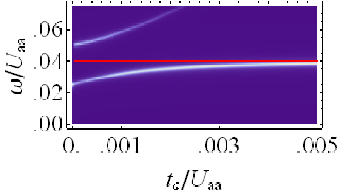
The $f_{n}$’s are found at each point in the phase diagram by starting with a trial $\alpha$, solving Eq. (13), then updating $\alpha$ via Eq. (14) and iterating. We find that almost all spectral weight typically lies in only one or two peaks. Fig. 2 shows sample spectra. The superfluid near the Mott state displays a multi-modal spectrum, but in the weakly interacting limit only a single peak is seen. An avoided crossing is clearly visible in these plots. Fig. 3 shows the manifold of spectral peaks in the $t_{a}/U_{aa}$ and $\mu/U_{aa}$ plane, using height to denote frequency and opacity to denote spectral weight. Taking moments of $\chi^{R}(\omega)$, we see that Eq. (8) is satisfied.

Although finding the spectrum in Eq. (22) is a trivial numerical task, one can gain further insight by considering limiting cases. First, when $U_{ab}=U_{aa}$ and $t_{a}=t_{b}$ the system possesses an $SU(2)$ symmetry. In this limit we find that $G_{n}(t)=-i\sqrt{n}f_{n}\theta(t)$ is constant for $t>0$. Thus our approximation gives a spectrum $I(\omega)$ which is proportional to $\delta(\omega)$. This result coincides with the exact behavior of the system: the operator $X=\sum_{j}b_{j}^{\dagger}a_{j}$ is a ladder operator, $[H,X]=\delta X$, and can only generate excitations with energy $\delta$ (set equal to zero in our calculation). The fact that our approximations correctly capture this behavior is nontrivial: in a field theoretic language one would say that our equation of motion approach includes the vertex corrections necessary for satisfying the relevant “Ward identities” [22, 23, 24].

The current ⁸⁷Rb experiments are slightly perturbed from this limit, with $\eta\equiv(U_{ab}-U_{aa})/U_{aa}\approx-0.025$ and $t_{b}=t_{a}$. We find that the $\delta$-function is shifted by a frequency proportional to $\eta$, but that the total spectral weight remains concentrated on that one frequency: the sum of the spectral weights at all other frequencies scale as $\eta^{2}$. Consequently it is an excellent approximation to treat the spectrum as a delta-function, and our RPA calculation reduces to the results in [5]. We emphasize however that other atoms, such as Cesium, can be in a regime where $\eta$ is large.

We gain further insight by considering the superfluid near the Mott phase with $t_{a}/U_{a}\ll 1$. Here one can truncate the basis to two states with total particle number $n$ and $n+1$ on each site. Then the $f_{n}$’s and $G_{n}$’s can be found analytically: one only needs to solve $2\times 2$ linear algebra problems. In the $t_{b}=0$, $U_{ab}=U_{aa}$ limit, this is similar to Ref. [6]’s approach, but includes the hopping self consistently, allowing us to satisfy the sum rule Eq. (8). This truncation is exact in the small $t_{a}$ limit, and yields

$\displaystyle\chi^{(R)}(\omega)$

$\displaystyle=$

$\displaystyle A_{+}\delta(\omega-\omega_{+})+A_{-}\delta(\omega-\omega_{-})$

(23)

with

$\displaystyle\omega_{\pm}=$

$\displaystyle\frac{\epsilon_{1}+\epsilon_{2}}{2}\pm\sqrt{\Delta^{2}+\left(\frac{\epsilon_{1}-\epsilon_{2}}{2}\right)^{2}}$

(24)

where

	$\displaystyle\epsilon_{1}$	$\displaystyle\equiv$	$\displaystyle(U_{ab}-U_{aa})(n-1)+zt_{a}f_{n+1}^{2}(n+1)$
	$\displaystyle\epsilon_{2}$	$\displaystyle\equiv$	$\displaystyle(U_{ab}-U_{aa})n+z\left[t_{a}(n+1)-t_{b}\right]f_{n}^{2}$
	$\displaystyle\Delta$	$\displaystyle\equiv$	$\displaystyle-\sqrt{n(n+1)}t_{a}zf_{n}f_{n+1}.$		(25)

if $n\geq 1$ and

	$\displaystyle\epsilon_{1}$	$\displaystyle\equiv$	$\displaystyle zt_{a}f_{1}^{2}$
	$\displaystyle\epsilon_{2}$	$\displaystyle\equiv$	$\displaystyle z(t_{a}-t_{b})f_{0}^{2}$
	$\displaystyle\Delta$	$\displaystyle\equiv$	$\displaystyle 0.$		(26)

if $n=0$ (here, only the $\epsilon_{2}$ peak has non-zero spectral weight). We omit the cumbersome analytic expressions for the spectral weights $A_{\pm}$. The spectrum consist of two peaks – hybridized versions of the excitations caricatured in Fig. 1. One can identify $\epsilon_{1}$ and $\epsilon_{2}$ as the energies of those caricature processes, recognizing that the hybridization term, $\Delta$, grows with $t_{a}$. The avoided crossing between these modes is evident in Fig. 2.

We model the trapped spectrum through a local density approximation. We assume that a given point in the trap has the properties of a homogeneous gas with chemical potential $\mu(r)=\mu_{0}-V(r)$. In Fig. 4 we show the density profile and the spectrum corresponding to each point in space. Also shown is the trap averaged spectrum. The bimodality of the homogeneous spectrum is quite effectively washed out by the inhomogeneous broadening of the trap. On the other hand, if one images the atoms flipped into the $b$ state as in Ref. [3], there is a clear qualitative signature of the bimodality. If one excites the system with an RF pulse whose frequency lies between the resonant frequencies of two Mott plateaus, one will excite two “shells” of atoms. These shells should be clearly visible, even in column integrated data.

References

- [1] D. Jaksch, C. Bruder, J. I. Cirac, C. W. Gardiner, and P. Zoller, Phys. Rev. Lett. 81, 3108 (1998).
- [2] M. P. A. Fisher, P. B. Weichman, G. Grinstein, and D. S. Fisher, Phys. Rev. B 40, 546 (1989).
- [3] G. K. Campbell, J. Mun, M. Boyd, P. Medley, A. E. Leanhardt, L. G. Marcassa, D. E. Pritchard, and W. Ketterle, Science 313, 649 (2006).
- [4] I. Bloch, J. Dalibard, and W. Zwerger, Reviews of Modern Physics 80, 885 (2008).
- [5] K. R. A. Hazzard and E. J. Mueller, Phys. Rev. A 76, 063612 (2007).
- [6] K. Sun, C. Lannert, and S. Vishveshwara, Phys. Rev. A 79, 043422 (2009).
- [7] D. G. Fried, T. C. Killian, L. Willmann, D. Landhuis, S. C. Moss, D. Kleppner, and T. J. Greytak, Phys. Rev. Lett. 81, 3811 (1998).
- [8] Y. Ohashi, M. Kitaura, and H. Matsumoto, Phys. Rev. A 73, 033617 (2006).
- [9] M. O. Oktel and L. S. Levitov, Phys. Rev. Lett. 83, 6 (1999).
- [10] I. H. Deutsch and P. S. Jessen, Phys. Rev. A 57, 1972 (1998).
- [11] L. Pollet, S. Rombouts, K. Heyde, and J. Dukelsky, Phys. Rev. A 69, 043601 (2004).
- [12] S. Bergkvist, P. Henelius, and A. Rosengren, Phys. Rev. A 70, 053601 (2004).
- [13] S. Wessel, F. Alet, M. Troyer, and G. G. Batrouni, Phys. Rev. A 70, 053615 (2004).
- [14] G. G. Batrouni, V. Rousseau, R. T. Scalettar, M. Rigol, A. Muramatsu, P. J. H. Denteneer, and M. Troyer, Phys. Rev. Lett. 89, 117203 (2002).
- [15] B. DeMarco, C. Lannert, S. Vishveshwara, and T.-C. Wei, Phys. Rev. A 71, 063601 (2005).
- [16] N. Dupuis and K. Sengupta, Physica B: Condensed Matter 404, 517 (2009).
- [17] K. Sengupta and N. Dupuis, Phys. Rev. A 71, 033629 (2005).
- [18] S. Konabe, T. Nikuni, and M. Nakamura, Phys. Rev. A 73, 033621 (2006).
- [19] C. Menotti and N. Trivedi, Phys. Rev. B 77, 235120 (2008).
- [20] M. O. Oktel, T. C. Killian, D. Kleppner, and L. S. Levitov, Phys. Rev. A 65, 033617 (2002).
- [21] M. O. Oktel and L. S. Levitov, Phys. Rev. Lett. 83, 6 (1999).
- [22] C. J. Pethick and H. T. C. Stoof, Phys. Rev. A 64, 013618 (2001).
- [23] G. Baym, Phys. Rev. 127, 1391 (1962).
- [24] J. Zinn-Justin, Quantum field theory and critical phenomena (Oxford University Press, Oxford University Press Inc., New York, 2002).
- [25] J. T. Stewart, J. P. Gaebler, and D. S. Jin, Nature 454, 744 (2008).