From Spectrum Pooling to Space Pooling: Opportunistic Interference Alignment in MIMO Cognitive Networks

S.M. Perlaza N. Fawaz S. Lasaulce and M. Debbah ^†^†thanks: S.M. Perlaza is with Orange Labs, France Telecom R&D. $38-40$ rue du Général Leclerc, 92794, Issy les Moulineaux, cedex $9$. France. (samir.medinaperlaza@orange-ftgroup.com)^†^†thanks: N.˜Fawaz is with the Research Laboratory of Electronics, Massachusetts Institute of Technology (MIT). Cambridge, Massachusetts, MA-02139, USA. (nfawaz@mit.edu). ^†^†thanks: S. Lasaulce is with LSS (CNRS-SUPELEC-Paris Sud). $3$ rue Joliot-Curie, $91192$, Gif-sur-Yvette, cedex. France. (lasaulce@lss.supelec.fr) ^†^†thanks: M. Debbah is with Alcatel-Lucent Chair in Flexible Radio at SUPELEC. $3$ rue Joliot-Curie, $91192$, Gif-sur-Yvette, cedex. France. (merouane.debbah@supelec.fr)^†^†thanks: The material in this paper has been presented in part at PIMRC 2008. September 2008, Cannes, France [1].

Abstract

We describe a non-cooperative interference alignment (IA) technique which allows an opportunistic multiple input multiple output (MIMO) link (secondary) to harmlessly coexist with another MIMO link (primary) in the same frequency band. Assuming perfect channel knowledge at the primary receiver and transmitter, capacity is achieved by transmiting along the spatial directions (SD) associated with the singular values of its channel matrix using a water-filling power allocation (PA) scheme. Often, power limitations lead the primary transmitter to leave some of its SD unused. Here, it is shown that the opportunistic link can transmit its own data if it is possible to align the interference produced on the primary link with such unused SDs. We provide both a processing scheme to perform IA and a PA scheme which maximizes the transmission rate of the opportunistic link. The asymptotes of the achievable transmission rates of the opportunistic link are obtained in the regime of large numbers of antennas. Using this result, it is shown that depending on the signal-to-noise ratio and the number of transmit and receive antennas of the primary and opportunistic links, both systems can achieve transmission rates of the same order.

I Introduction

The concept of cognitive radio is well-known by now. The main idea is to let a class of radio devices, called secondary systems, opportunistically access certain portions of spectrum left unused by other radio devices, called primary systems, at a given time or geographical area [2]. These pieces of unused spectrum, known as white-spaces, appear mainly when either transmissions in the primary network are sporadic, i.e., there are periods over which no transmission takes place, or there is no network infrastructure for the primary system in a given area, for instance, when there is no primary network coverage in a certain region. In the case of dense networks, a white-space might be a rare and short-lasting event. As a matter of fact, the idea of cognitive radio as presented in [2] (i.e., spectrum pooling), depends on the existence of such white-spaces [3]. In the absence of those spectrum holes, secondary systems are unable to transmit without producing additional interference on the primary systems. One solution to this situation has been provided recently under the name of interference alignment (IA) [4]. Basically, IA refers to the construction of signals such that the resulting interference signal lies in a subspace orthogonal to the one spanned by the signal of interest at each receiver [5]. The IA concept was introduced separetely and almost simultaneously by several authors [6, 7, 4, 8]. Recently, IA has become an important tool to study the interference channel, namely its degrees of freedom [5, 4, 9]. The feasibility and implementation issues of IA regarding mainly the required channel state information (CSI) has been also extensively studied [10, 11, 12, 13].

In this paper we study an IA scheme named opportunistic IA (OIA) [1]. The idea behind OIA can be briefly described as follows. The primary link is modeled by a single-user MIMO channel since it must operate free of any additional interference produced by secondary systems. Then, assuming perfect CSI at both transmitter and receiver ends, capacity is achieved by implementing a water-filling power allocation (PA) scheme [14] over the spatial directions associated with the singular values of its channel transfer matrix. Interestingly, even if the primary transmitters maximize their transmission rates, power limitations generally lead them to leave some of their spatial directions (SD) unused. The unused SD can therefore be reused by another system operating in the same frequency band. Indeed, an opportunistic transmitter can send its own data to its respective receiver by processing its signal in such a way that the interference produced on the primary link impairs only the unused SDs. Hence, these spatial resources can be very useful for a secondary system when the available spectral resources are fully exploited over a certain period in a geographical area. The idea of OIA, as described above, was first introduced in [1] considering a very restrictive scenario, e.g., both primary and secondary devices have the same number of antennas and same power budget. In this paper, we consider a more general framework where devices have different number of antennas, different power budgets and no conditions are impossed over the channel transfer matrices (In [1], full rank condition was impossed over certain matrices).

The rest of this paper is structured as follows. First, the system model, which consists of an interference channel with MIMO links, is introduced in Sec. II. Then, our aim in Sec. III is twofold. First, an analysis of the feasibility of the OIA scheme is provided. For this purpose, the existence of transmit opportunities (SD left unused by the primary system) is studied. The average number of transmit opportunities is expressed as a function of the number of antennas at both the primary and secondary terminals. Second, the proposed interference alignment technique and power allocation (PA) policy at the secondary transmitter are described. In Sec. IV-B, tools from random matrix theory for large systems are used to analyze the achievable transmission rate of the opportunistic transmitter when no optimization is performed over its input covariance matrix. We illustrate our theoretical results by simulations in Sec. V. Therein, it is shown that our approach allows the secondary link to achieve transmission rates of the same order as those of the primary link. Finally, in Sec. VI we state our conclusions and provide possible extensions of this work.

II System Model

Notations. In the sequel, matrices and vectors are respectively denoted by boldface upper case symbols and boldface lower case symbols. An $N\times K$ matrix with ones on its main diagonal and zeros on its off-diagonal entries is denoted by ${\bf I}_{N\times K}$ , while the identity matrix of size $N$ is simply denoted by ${\bf I}_{N}$ . An $N\times K$ matrix with zeros in all its entries (null matrix) is denoted by $\mathbf{0}_{N\times K}$ . Matrices $\mathbf{X}^{T}$ and $\mathbf{X}^{H}$ are the transpose and Hermitian transpose of matrix $\mathbf{X}$ , respectively. The determinant of matrix $\mathbf{X}$ is denoted by $|\mathbf{X}|$ . The expectation operator is denoted by $\mathbb{E}\left[.\right]$ . The indicator function associated with a given set $\mathcal{A}$ is denoted by $\mathds{1}_{\mathcal{A}}(.)$ , and defined by $\mathds{1}_{\mathcal{A}}(x)=1$ (resp. $0$ ) if $x\in\mathcal{A}$ (resp. $x\notin\mathcal{A}$ ). The Heaviside step function and the Dirac delta function are respectively denoted by $\mu(\cdot)$ and $\delta(\cdot)$ . The symbols $\mathds{N}$ , $\mathds{R}$ , and $\mathds{C}$ denote the sets of non-negative integers, real numbers, and complex numbers, respectively. The subsets $\left[0,+\infty\right[$ and $\left]-\infty,0\right]$ are denoted by $\mathds{R}^{+}$ and $\mathds{R}^{-}$ , respectively. The operator $\left(x\right)^{+}$ with $x\in\mathds{R}$ is equivalent to the operation $\max\left(0,x\right)$ . Let $\mathbf{A}$ be an $n\times n$ square matrix with real eigenvalues $\lambda_{A,1},\ldots,\lambda_{A,n}$ . We define the empirical eigenvalue distribution of $\mathbf{A}$ by $F_{A}^{(n)}(\cdot)\triangleq\frac{1}{n}\sum_{i=1}^{n}\mu(\lambda-\lambda_{A,i})$ , and, when it exists, we denote $f_{A}^{(n)}(\lambda)$ the associated eigenvalue probability density function, where $F_{\mathbf{A}}(\cdot)$ and $f_{\mathbf{A}}(\cdot)$ are respectively the associated limiting eigenvalue distribution and probability density function when $n\rightarrow+\infty$ .

We consider two unidirectional links simultaneously operating in the same frequency band and producing mutual interference as shown in Fig. 1. The first transmitter-receiver pair $(\mathrm{Tx}_{1},\mathrm{Rx}_{1})$ is the primary link. The pair $(\mathrm{Tx}_{2},\mathrm{Rx}_{2})$ is an opportunistic link subject to the strict constraint that the primary link must transmit at a rate equivalent to its single-user capacity. Denote by $N_{i}$ and $M_{i}$ , with $i=1$ (resp. $i=2$ ), the number of antennas at the primary (resp. secondary) receiver and transmitter, respectively. Each transmitter sends independent messages only to its respective receiver and no cooperation between them is allowed, i.e., there is no message exchange between transmitters. This scenario is known as the MIMO interference channel (IC) [15, 16] with private messages. A private message is a message from a given source to a given destination: only one destination node is able to decode it. Indeed, we do not consider the case of common messages which would be generated by a given source in order to be decoded by several destination nodes.

In this paper, we assume the channel transfer matrices between different nodes to be fixed over the whole duration of the transmission. The channel transfer matrix from transmitter $j\in\left\{1,2\right\}$ to receiver $i\in\left\{1,2\right\}$ is an $N_{i}\times M_{j}$ matrix denoted by $\mathbf{H}_{ij}$ which corresponds to the realization of a random matrix with independent and identically distributed (i.i.d.) complex Gaussian circularly symmetric entries with zero mean and variance $\frac{1}{M_{j}}$ , which implies

\forall(i,j)\in\{1,2\}^{2},\quad\mathrm{Trace}\left(\mathds{E}\left[\mathbf{H}_{ij}\>\mathbf{H}_{ij}^{H}\right]\right)=N_{i}.

(1)

The $L_{i}$ symbols transmitter $i$ is able to simultaneously transmit, denoted by $s_{i,1},\ldots,s_{i,L_{i}}$ , are represented by the vector $\mathbf{s}_{i}=\left(s_{i,1},\ldots,s_{i,L_{i}}\right)^{T}$ . We assume that $\forall i\in\{1,2\}$ symbols $s_{i,1},\ldots,s_{i,L_{i}}$ are i.i.d. zero-mean circularly-symmetric complex Gaussian variables. In our model, transmitter $i$ processes its symbols using a matrix $\mathbf{V}_{i}$ to construct its transmitted signal $\mathbf{V}_{i}\mathbf{s}_{i}$ . Therefore, the matrix $\mathbf{V}_{i}$ is called pre-processing matrix. Following a matrix notation, the primary and secondary received signals, represented by the $N_{i}\times 1$ column-vectors $\mathbf{r}_{i}$ , with $i\in\{1,2\}$ , can be written as

\left(\begin{array}[]{c}\mathbf{r}_{1}\\ \mathbf{r}_{2}\end{array}\right)=\left(\begin{array}[]{cc}\mathbf{H}_{11}&\mathbf{H}_{12}\\ \mathbf{H}_{21}&\mathbf{H}_{22}\end{array}\right)\left(\begin{array}[]{c}\mathbf{V}_{1}\mathbf{s}_{1}\\ \mathbf{V}_{2}\mathbf{s}_{2}\end{array}\right)+\left(\begin{array}[]{c}\mathbf{n}_{1}\\ \mathbf{n}_{2}\end{array}\right),

(2)

where $\mathbf{n}_{i}$ is an $N_{i}$ -dimensional vector representing noise effects at receiver $i\in\{1,2\}$ with entries modeled by an additive white Gaussian noise (AWGN) process with zero mean and variance $\sigma^{2}_{i}$ , i.e., $\forall i\in\{1,2\}$ , $\mathbb{E}\left[\mathbf{n}_{i}\mathbf{n}_{i}^{H}\right]=\sigma^{2}_{i}{\bf I}_{N_{i}}$ . At transmitter $i\in\{1,2\}$ , the $L_{i}\times L_{i}$ power allocation matrix $\mathbf{P}_{i}$ is defined by the input covariance matrix $\mathbf{P}_{i}=\mathbb{E}\left[\mathbf{s}_{i}\mathbf{s}_{i}^{H}\right]$ . Note that symbols $s_{i,1}\ldots,s_{i,L_{i}}$ , $\forall i\in\{1,2\}$ are mutually independent and zero-mean, thus, the PA matrices can be written as diagonal matrices, i.e., $\mathbf{P}_{i}={\mathrm{diag}}\left(p_{i,1},\ldots,p_{i,L_{i}}\right)$ . Choosing $\mathbf{P}_{i}$ therefore means selecting a given PA policy. The power constraints on the transmitted signals $\mathbf{V}_{i}\mathbf{s}_{i}$ can be written as

\forall i\in\left\{1,2\right\},\quad\text{Trace}\left(\mathbf{V}_{i}\mathbf{P}_{i}\mathbf{V}_{i}^{H}\right)\leqslant M_{i}\>p_{i,\max}.

(3)

Note that assuming that the i.i.d. entries of matrices $\mathbf{H}_{ij}$ , for all $(i,j)\in\left\{1,2\right\}^{2}$ , are Gaussian random variables with zero mean and variance $\frac{1}{M_{j}}$ , together with the power constraints in (3), is equivalent to considering a system where the entries of matrices $\mathbf{H}_{ij}$ for all $(i,j)\in\left\{1,2\right\}^{2}$ are Gaussian random variables with zero mean and unit variance, and the transmitted signal $\mathbf{V}_{i}\mathbf{s}_{i}$ are constrained by a finite transmit power $p_{i,\max}$ . Nonetheless, the second convention allows us to increase the dimension of the system (number of antennas) while maintaining the same average received signal to noise ratio (SNR) level $\frac{p_{i,\max}}{\sigma_{i}^{2}}$ , $\forall i\in\left\{1,2\right\}$ . Moreover, most of the tools from random matrix theory used in the asymptotic analysis of the achievable data rate of the opportunistic link in Sec. IV-B, require the variance of the entries of channel matrices to be normalized by its size. That is the reason why the normalized model, i.e., channel transfer matrices and power constraints respectively satisfying (1) and (3), was adopted.

At receiver $i\in\left\{1,2\right\}$ , the signal $\mathbf{r}_{i}$ is processed using an $N_{i}\times N_{i}$ matrix $\mathbf{D}_{i}$ to form the $N_{i}$ -dimensional vector $\mathbf{y}_{i}=\mathbf{D}_{i}\mathbf{r}_{i}$ . All along this paper, we refer to $\mathbf{D}_{i}$ as the post-processing matrix at receiver $i$ . Regarding channel knowledge assumptions at the different nodes, we assume that the primary terminals (transmitter and receiver) have perfect knowledge of the matrix $\mathbf{H}_{11}$ while the secondary terminals have perfect knowledge of all channel transfer matrices $\mathbf{H}_{ij}$ , $\forall(i,j)\in\left\{1,2\right\}^{2}$ . One might ask whether this setup is highly demanding in terms of information assumptions. In fact, there are several technical arguments making this setup relatively realistic: (a) in some contexts channel reciprocity can be exploited to acquire CSI at the transmitters; (b) feedback channels are often available in wireless communications [11], and (c) learning mechanisms [12] can be exploited to iteratively learn the required CSI. In any case, the perfect information assumptions provide us with an upper bound on the achievable transmission rate for the secondary link.

III Interference Alignment Strategy

In this section, we describe how both links introduced in Sec. II can simultaneously operate under the constraint that no additional interference is generated by the opportunistic transmitter on the primary receiver. First, we revisit the transmitting scheme implemented by the primary system [14], then we present the concept of transmit opportunity, and finally we introduce the proposed opportunistic IA technique.

III-A Primary Link Performance

According to our initial assumptions (Sec. II) the primary link must operate at its highest transmission rate in the absence of interference. Hence, following the results in [14, 17] and using our own notation, the optimal pre-processing and post-processing schemes for the primary link are given by the following theorem.

Theorem 1

Let $\mathbf{H}_{11}=\mathbf{U}_{H_{11}}\mathbf{\Lambda}_{H_{11}}\mathbf{V}^{H}_{H_{11}}$ be a singular value decomposition (SVD) of the $N_{1}\times M_{1}$ channel transfer matrix $\mathbf{H}_{11}$ , with $\mathbf{U}_{H_{11}}$ and $\mathbf{V}_{H_{11}}$ , two unitary matrices with dimension $N_{1}\times N_{1}$ and $M_{1}\times M_{1}$ , respectively, and $\mathbf{\Lambda}_{H_{11}}$ an $N_{1}\times M_{1}$ matrix with main diagonal $\left(\lambda_{H_{11},1},\ldots,\lambda_{H_{11},\min(N_{1},M_{1})}\right)$ and zeros on its off-diagonal. The primary link achieves capacity by choosing $\mathbf{V}_{1}=\mathbf{V}_{H_{11}}$ , $\mathbf{D}_{1}=\mathbf{U}_{H_{11}}^{H}$ , $\mathbf{P}_{1}={\mathrm{diag}}{\left(p_{1,1},\ldots,p_{1,M_{1}}\right)}$ , where

\forall n\in\left\{1,\ldots,M_{1}\right\},\quad p_{1,n}=\left(\beta-\frac{\sigma^{2}_{1}}{\lambda_{H_{11}^{H}H_{11},n}}\right)^{+},

(4)

with, $\mathbf{\Lambda}_{H_{11}^{H}H_{11}}=\mathbf{\Lambda}_{H_{11}}^{H}\mathbf{\Lambda}_{H_{11}}={\mathrm{diag}}\left(\lambda_{H_{11}^{H}H_{11},1},\ldots,\lambda_{H_{11}^{H}H_{11},M_{1}}\right)$ and the constant $\beta$ (water-level) is set to saturate the power constraint (3).

Let $N\triangleq\min(N_{1},M_{1})$ . When implementing its capacity-achieving transmission scheme, the primary transmitter allocates its transmit power over an equivalent channel $\mathbf{D}_{1}\mathbf{H}_{11}\mathbf{V}_{1}=\mathbf{\Lambda}_{H_{11}}$ which consists of at most ${\mathrm{rank}}(\mathbf{H}_{11}^{H}\mathbf{H}_{11})\leq N$ parallel sub-channels with non-zero channel gains $\lambda_{H_{11}^{H}H_{11},n}$ , respectively. These non-zero channel gains to which we refer as transmit dimensions, correspond to the non-zero eigenvalues of matrix $\mathbf{H}_{11}^{H}\mathbf{H}_{11}$ . The transmit dimension $n\in\{1,\ldots,M_{1}\}$ is said to be used by the primary transmitter if $p_{1,n}>0$ . Interestingly, (4) shows that some of the transmit dimensions can be left unused. Let $m_{1}\in\{1,\ldots,M_{1}\}$ denote the number of transmit dimensions used by the primary user:

\begin{split}m_{1}&\triangleq\sum_{n=1}^{M_{1}}{\mathds{1}}_{]0,M_{1}p_{\mathrm{1,\max}}]}(p_{1,n})\\ &=\sum_{n=1}^{M_{1}}\mathds{1}_{\left]\frac{\sigma^{2}_{1}}{\beta},+\infty\right[}(\lambda_{H_{11}^{H}H_{11},n}).\end{split}

(5)

As $p_{\mathrm{1,\max}}>0$ , the primary link transmits at least over dimension $n^{*}=\displaystyle\arg\max_{m\in\{1,\ldots,\min(N_{1},M_{1})\}}\left\{\lambda_{H_{11}^{H}H_{11},m}\right\}$ regardless of its SNR, and moreover, there exist at most $N$ transmit dimensions, thus

1\leq m_{1}\leq{\mathrm{rank}}(\mathbf{H}_{11}^{H}\mathbf{H}_{11})\leq N.

(6)

In the following section, we show how those unused dimensions of the primary system can be seen by the secondary system as opportunities to transmit.

III-B Transmit Opportunities

Once the PA matrix is set up following Th. 1, the primary equivalent channel $\mathbf{D}_{1}\mathbf{H}_{11}\mathbf{V}_{1}\mathbf{P}_{1}^{1/2}=\mathbf{\Lambda}_{H_{11}}\mathbf{P}_{1}^{1/2}$ is an $N_{1}\times M_{1}$ diagonal matrix whose main diagonal contains $m_{1}$ non-zero entries and $N-m_{1}$ zero entries. This equivalent channel transforms the set of $m_{1}$ used and $M_{1}-m_{1}$ unused transmit dimensions into a set of $m_{1}$ receive dimensions containing a noisy version of the primary signal, and a set of $N_{1}-m_{1}$ unused receive dimensions containing no primary signal. The $m_{1}$ useful dimensions are called primary reserved dimensions, while the remaining $N_{1}-m_{1}$ dimensions are named secondary transmit opportunities (TO). The IA strategy, described in Section III-C, allows the secondary user to exploit these $N_{1}-m_{1}$ receive dimensions left unused by the primary link, while avoiding to interfere with the $m_{1}$ receive dimensions used by the primary link.

Definition 2 (Transmit Opportunities)

Let $\lambda_{H_{11}^{H}H_{11},1},\ldots\lambda_{H_{11}^{H}H_{11},M_{1}}$ be the eigenvalues of matrix $\mathbf{H}_{11}^{H}\mathbf{H}_{11}$ and $\beta$ be the water-level in (Th. 1). Let $m_{1}$ , as defined in (5), be the number of primary reserved dimensions. Then the number of transmit opportunities $S$ available to the opportunistic terminal is given by

S\triangleq N_{1}-m_{1}=N_{1}-\sum_{n=1}^{M_{1}}\mathds{1}_{\left]\frac{\sigma^{2}_{1}}{\beta},+\infty\right[}(\lambda_{H_{11}^{H}H_{11},n}).

(7)

Note that in this definition it is implicitly assumed that the number of TOs is constant over a duration equal to the channel coherence time.

Combining (6) and (7) yields the bounds on the number of transmit opportunities

N_{1}-N\leq S\leq N_{1}-1.

(8)

A natural question arises as to whether the number of TOs is sufficiently high for the secondary link to achieve a significant transmission rate. In order to provide an element of response to this question, a method to find an approximation of the number of TOs per primary transmit antenna, $S_{\infty}$ , is proposed in Section IV-A. In any case, as we shall see in the next section, to take advantage of the TOs described in this section, a specific signal processing scheme is required in the secondary link.

III-C Pre-processing Matrix

In this section, we define the interference alignment condition to be met by the secondary transmitter and determine a pre-processing matrix satisfying this condition.

Definition 3 (IA condition)

Let $\mathbf{H}_{11}=\mathbf{U}_{H_{11}}\mathbf{\Lambda}_{H_{11}}\mathbf{V}_{H_{11}}^{H}$ be an SVD of $\mathbf{H}_{11}$ and

\displaystyle\mathbf{R}

\displaystyle=

\displaystyle\sigma^{2}_{1}{\bf I}_{N_{1}}+\mathbf{U}_{H_{11}}^{H}\mathbf{H}_{12}\mathbf{V}_{2}\mathbf{P}_{2}\mathbf{V}_{2}^{H}\mathbf{H}_{12}^{H}\mathbf{U}_{H_{11}},

(9)

be the covariance matrix of the co-channel interference (CCI) plus noise signal in the primary link. The opportunistic link is said to satisfy the IA condition if its opportunistic transmission is such that the primary link achieves the transmission rate of the equivalent single-user system, which translates mathematically as

\begin{array}[]{lcl}\log_{2}\left|{\bf I}_{N_{1}}+\frac{1}{\sigma^{2}_{1}}\mathbf{\Lambda}_{H_{11}}\mathbf{P}_{1}\mathbf{\Lambda}_{H_{11}}^{H}\right|=&&\\ \log_{2}\left|{\bf I}_{N_{1}}+\mathbf{R}^{-1}\mathbf{\Lambda}_{H_{11}}\mathbf{P}_{1}\mathbf{\Lambda}_{H_{11}}^{H}\right|.&&\end{array}

(10)

Our objective is first to find a pre-processing matrix $\mathbf{V}_{2}$ that satisfies the IA condition and then, to tune the PA matrix $\mathbf{P}_{2}$ and post-processing matrix $\mathbf{D}_{2}$ in order to maximize the transmission rate for the secondary link.

Lemma 1 (Pre-processing matrix $\mathbf{V}_{2}$ )

Let $\mathbf{H}_{11}=\mathbf{U}_{H_{11}}\mathbf{\Lambda}_{H_{11}}\mathbf{V}_{H_{11}}^{H}$ be an ordered SVD of $\mathbf{H}_{11}$ , with $\mathbf{U}_{H_{11}}$ and $\mathbf{V}_{H_{11}}$ , two unitary matrices of size $N_{1}\times N_{1}$ and $M_{1}\times M_{1}$ , respectively, and $\mathbf{\Lambda}_{H_{11}}$ an $N_{1}\times M_{1}$ matrix with main diagonal $\left(\lambda_{H_{11},1},\ldots,\lambda_{H_{11},\min(N_{1},M_{1})}\right)$ and zeros on its off-diagonal, such that $\lambda_{H_{11},1}^{2}\geqslant\lambda_{H_{11},2}^{2}\geqslant\ldots\geqslant\lambda_{H_{11},\min(N_{1},M_{1})}^{2}$ . Let also the $N_{1}\times M_{2}$ matrix $\tilde{\mathbf{H}}\stackrel{{\scriptstyle\triangle}}{{=}}\mathbf{U}_{H_{11}}^{H}\mathbf{H}_{12}$ have a block structure,

\tilde{\mathbf{H}}=\begin{array}[]{rc}&{\mathrel{\to}^{M_{2}}}\\ \begin{array}[]{r}m_{1}\Big\updownarrow\\ N_{1}-m_{1}\Big\updownarrow\end{array}&\left(\begin{array}[]{c}\tilde{\mathbf{H}}_{1}\\ \tilde{\mathbf{H}}_{2}\end{array}\right)\end{array}.

(11)

The IA condition (Def. 3) is satisfied independently of the PA matrix $\mathbf{P}_{2}$ , when the pre-processing matrix $\mathbf{V}_{2}$ satisfies the condition:

\tilde{\mathbf{H}}_{1}\mathbf{V}_{2}=\mathbf{0}_{m_{1}\times L_{2}},

(12)

where $L_{2}$ is the dimension of the null space of matrix $\tilde{\mathbf{H}}_{1}$ .

Proof:

See Appendix A. ∎Another solution to the IA condition was given in [1], namely $\mathbf{V}_{2}=\mathbf{H}_{12}^{-1}\mathbf{U}_{H_{11}}\bar{\mathbf{P}}_{1}$ for a given diagonal matrix $\bar{\mathbf{P}}_{1}={\mathrm{diag}}\left(\bar{p}_{1,1},\ldots,\bar{p}_{1,M_{1}}\right)$ , with $\bar{p}_{1,n}=\left(\frac{\sigma^{2}_{2}}{\lambda_{H_{11}^{H}H_{11},n}}-\beta\right)^{+}$ , where $\beta$ is the water-level of the primary system (Th. 1) and $n\in\{1,\ldots,M_{1}\}$ . However, such a solution is more restrictive than (12) since it requires $\mathbf{H}_{12}$ to be invertible and does not hold for the case when $N_{i}\neq M_{j}$ , $\forall(i,j)\in\{1,2\}^{2}$ .

Plugging $\mathbf{V}_{2}$ from (12) into (9) shows that to guarantee the IA condition (3), the opportunistic transmitter has to avoid interfering with the $m_{1}$ dimensions used by the primary transmitter. That is the reason why we refer to our technique as OIA: interference from the secondary user is made orthogonal to the $m_{1}$ receive dimensions used by the primary link. This is achieved by aligning the interference from the secondary user with the $N_{1}-m_{1}$ non-used receive dimensions of the primary link.

From Lemma 1, it appears that the $L_{2}$ columns of matrix $\mathbf{V}_{2}$ have to belong to the null space ${\mathrm{Ker}}(\tilde{\mathbf{H}}_{1})$ of $\tilde{\mathbf{H}}_{1}$ and therefore to the space spanned by the $\dim{\mathrm{Ker}}(\tilde{\mathbf{H}}_{1})=M_{2}-{\mathrm{rank}}(\tilde{\mathbf{H}}_{1})$ last columns of matrix $\mathbf{V}_{\tilde{H}_{1}}$ , where $\tilde{\mathbf{H}}_{1}=\mathbf{U}_{\tilde{H}_{1}}\mathbf{\Lambda}_{\tilde{H}_{1}}\mathbf{V}_{\tilde{H}_{1}}^{H}$ is an SVD of $\mathbf{\tilde{H}}_{11}$ with $\mathbf{U}_{\tilde{H}_{1}}$ and $\mathbf{V}_{\tilde{H}_{1}}$ two unitary matrices of respective sizes $m_{1}\times m_{1}$ and $M_{2}\times M_{2}$ , and $\mathbf{\Lambda}_{\tilde{H}_{1}}$ an $m_{1}\times M_{2}$ matrix containing the vector $(\lambda_{\tilde{H}_{11},1},\ldots,\lambda_{\tilde{H}_{1},\min(m_{1},M_{2})})$ on its main diagonal and zeros on its off-diagonal, such that $\lambda_{\tilde{H}_{11},1}^{2}\geqslant\ldots\geqslant\lambda_{\tilde{H}_{1},\min(m_{1},M_{2})}^{2}$ . i.e.,

\mathbf{V}_{2}\in{\mathrm{Span}}\left(\mathbf{v}_{\tilde{H}_{1}}^{({\mathrm{rank}}(\tilde{\mathbf{H}}_{1})+1)},\ldots,\mathbf{v}_{\tilde{H}_{1}}^{(M_{2})}\right).

(13)

Here, for all $i\in\left\{1,\ldots,M_{2}\right\}$ , the column vector $\mathbf{v}_{\tilde{H}_{1}}^{(i)}$ represents the $i^{th}$ column of matrix $\mathbf{V}_{\tilde{H}_{1}}$ from the left to the right.

In the following, we assume that the $L_{2}$ columns of the matrix $\mathbf{V}_{2}$ form an orthonormal basis of the corresponding subspace (13), and thus, $\mathbf{V}_{2}^{H}\mathbf{V}_{2}={\bf I}_{L_{2}}$ . Moreover, recalling that $\tilde{\mathbf{H}}_{1}$ is of size $m_{1}\times M_{2}$ , we would like to point out that:

•

When $m_{1}<M_{2}$ , ${\mathrm{rank}}(\tilde{\mathbf{H}}_{1})\leq m_{1}$ and $\dim{\mathrm{Ker}}(\tilde{\mathbf{H}}_{1})\geq M_{2}-m_{1}$ with equality if and only if $\tilde{\mathbf{H}}_{1}$ is full row-rank. This means that there are always at least $M_{2}-m_{1}>0$ non-null orthogonal vectors in ${\mathrm{Ker}}(\tilde{\mathbf{H}}_{1})$ , and thus, $L_{2}=\dim{\mathrm{Ker}}(\tilde{\mathbf{H}}_{1})$ . Consequently, $\mathbf{V}_{2}$ can always be chosen to be different from the null matrix $\mathbf{0}_{M_{2}\times L_{2}}$ .
•

When, $M_{2}\leqslant m_{1}$ , ${\mathrm{rank}}(\mathbf{\tilde{H}}_{1})\leq M_{2}$ and $\dim{\mathrm{Ker}}(\mathbf{\tilde{H}}_{1})\geq 0$ , with equality if and only if $\mathbf{\tilde{H}}_{1}$ is full column-rank. This means that there are non-zero vectors in ${\mathrm{Ker}}(\mathbf{\tilde{H}}_{1})$ if and only if $\mathbf{\tilde{H}}_{1}$ is not full column-rank. Consequently, $\mathbf{V}_{2}$ is a non-zero matrix if and only if $\mathbf{\tilde{H}}_{1}$ is not full column-rank, and again $L_{2}=\dim{\mathrm{Ker}}(\tilde{\mathbf{H}}_{1})$ .

Therefore, the rank of $\mathbf{V}_{2}$ is given by $L_{2}=\dim{\mathrm{Ker}}(\tilde{\mathbf{H}}_{1})\leq M_{2}$ , and it represents the number of transmit dimensions on which the secondary transmitter can allocate power without affecting the performance of the primary user. The following lower bound on $L_{2}$ holds

\begin{split}L_{2}=\dim{\mathrm{Ker}}(\tilde{\mathbf{H}}_{1})&=M_{2}-{\mathrm{rank}}(\tilde{\mathbf{H}}_{1})\\ &\geq M_{2}-\min(M_{2},m_{1})\\ &=\max(0,M_{2}-m_{1})\\ \end{split}

(14)

Note that by processing $\mathbf{s}_{2}$ with $\mathbf{V}_{2}$ the resulting signal $\mathbf{V}_{2}\mathbf{s_{2}}$ becomes orthogonal to the space spanned by a subset of $m_{1}$ rows of the cross-interference channel matrix $\tilde{\mathbf{H}}=\mathbf{U}_{H_{11}}^{H}\mathbf{H}_{12}$ . This is the main difference between the proposed OIA technique and the classical zero-forcing beamforming (ZFBF) [18], for which the transmit signal must be orthogonal to the whole row space of matrix $\tilde{\mathbf{H}}$ . In the ZFBF case, the number of transmit dimensions, on which the secondary transmitter can allocate power without affecting the performance of the primary user, is given by $L_{2,BF}=\dim{\mathrm{Ker}}(\tilde{\mathbf{H}})=M_{2}-{\mathrm{rank}}(\tilde{\mathbf{H}})$ . Since ${\mathrm{rank}}(\tilde{\mathbf{H}}_{1})\leq{\mathrm{rank}}(\tilde{\mathbf{H}})$ , we have $L_{2,BF}\leq L_{2}$ . This inequality, along with the observation that ${\mathrm{Ker}}(\tilde{\mathbf{H}})\subseteq{\mathrm{Ker}}(\tilde{\mathbf{H}}_{1})$ , shows that any opportunity to use a secondary transmit dimension provided by ZFBF is also provided by OIA, thus OIA outperforms ZFBF. In the next section we tackle the problem of optimizing the post-processing matrix $\mathbf{D}_{2}$ to maximize the achievable transmission rate for the opportunistic transmitter.

III-D Post-processing Matrix

Once the pre-processing matrix $\mathbf{V}_{2}$ has been adapted to perform IA according to (13), no harmful interference impairs the primary link. However, the secondary receiver undergoes the CCI from the primary transmitter. Then, the joint effect of the CCI and noise signals can be seen as a colored Gaussian noise with covariance matrix

\mathbf{Q}=\mathbf{H}_{21}\mathbf{V}_{H_{11}}\mathbf{P}_{1}\mathbf{V}_{H_{11}}^{H}\mathbf{H}_{21}^{H}+\sigma^{2}_{2}{\bf I}_{N_{2}}.

(15)

We recall that the opportunistic receiver has full CSI of all channel matrices, i.e., $\mathbf{H}_{i,j}$ , $\forall(i,j)\in\{1,2\}^{2}$ . Given an input covariance matrix $\mathbf{P}_{2}$ , the mutual information between the input $\mathbf{s}_{2}$ and the output $\mathbf{y}_{2}=\mathbf{D}_{2}\mathbf{r}_{2}$ is

	$\displaystyle\scriptstyle R_{2}(\mathbf{P}_{2},\sigma^{2}_{2})$	$\displaystyle=$	$\displaystyle\,\scriptstyle\log_{2}\left\|{\bf I}_{N_{2}}+\mathbf{D}_{2}\mathbf{H}_{22}\mathbf{V}_{2}\mathbf{P}_{2}\mathbf{V}_{2}^{H}\mathbf{H}_{22}^{H}\mathbf{D}_{2}^{H}\left(\mathbf{D}_{2}\mathbf{Q}\mathbf{D}_{2}^{H}\right)^{-1}\right\|$		(16)
		$\displaystyle\leqslant$	$\displaystyle\scriptstyle\log_{2}\left\|{\bf I}_{N_{2}}+\mathbf{Q}^{-\frac{1}{2}}\mathbf{H}_{22}\mathbf{V}_{2}\mathbf{P}_{2}\mathbf{V}_{2}^{H}\mathbf{H}_{22}^{H}\mathbf{Q}^{-\frac{1}{2}}\right\|,$		(16)

where equality is achieved by a whitening post-processing filter $\mathbf{D}_{2}=\mathbf{Q}^{-\frac{1}{2}}$ [19]. i.e., the mutual information between the transmitted signal $\mathbf{s}_{2}$ and $\mathbf{r}_{2}$ , is the same as that between $\mathbf{s}_{2}$ and $\mathbf{y}_{2}=\mathbf{D}_{2}\mathbf{r}_{2}$ . Note also that expression (16) is maximized by a zero-mean circularly-symmetric complex Gaussian input $\mathbf{s}_{2}$ [14].

III-E Power Allocation Matrix Optimization

In this section, we are interested in finding the input covariance matrix $\mathbf{P}_{2}$ which maximizes the achievable transmission rate for the opportunistic link, $R_{2}(\mathbf{P}_{2},\sigma^{2}_{2})$ assuming that both matrices $\mathbf{V}_{2}$ and $\mathbf{D}_{2}$ have been set up as discussed in Sec. III-C and III-D, respectively. More specifically, the problem of interest in this section is:

\begin{array}[]{lc}\displaystyle\max_{\mathbf{P}_{2}}&\scriptstyle\log_{2}\left|{\bf I}_{N_{2}}+\mathbf{Q}^{-\frac{1}{2}}\mathbf{H}_{22}\mathbf{V}_{2}\mathbf{P}_{2}\mathbf{V}_{2}^{H}\mathbf{H}_{22}^{H}\mathbf{Q}^{-\frac{1}{2}}\right|\\ \text{s.t.}&\scriptstyle\text{Trace}\left(\mathbf{V}_{2}\mathbf{P}_{2}\mathbf{V}_{2}^{H}\right)\leqslant p_{2,\mathrm{max}}.\end{array}

(17)

Before solving the optimization problem (OP) in (17), we briefly describe the uniform PA scheme (UPA). The UPA policy can be very useful not only to relax some information assumptions and decrease computational complexity at the transmitter but also because it corresponds to the limit of the optimal PA policy in the high SNR regime.

III-E1 Uniform Power Allocation

In this case, the opportunistic transmitter does not perform any optimization on its own transmit power. It rather uniformly spreads its total power among the previously identified TOs. Thus, the PA matrix $\mathbf{P}_{2}$ is assumed to be of the form

\mathbf{P}_{2,UPA}=\gamma{\bf I}_{L_{2}},

(18)

where the constant $\gamma$ is chosen to saturate the transmit power constraint (3),

\displaystyle\gamma=\frac{M_{2}\>p_{2,\max}}{{\mathrm{Trace}}\left(\mathbf{V}_{2}\mathbf{V}_{2}^{H}\right)}=\frac{M_{2}p_{2,\max}}{L_{2}}.

(19)

III-E2 Optimal Power Allocation

Here, we tackle the OP formulated in (17). For doing so, we assume that the columns of matrix $\mathbf{V}_{2}$ are unitary and mutually orthogonal. We define the matrix $\mathbf{K}\stackrel{{\scriptstyle\triangle}}{{=}}\mathbf{Q}^{-\frac{1}{2}}\mathbf{H}_{22}\mathbf{V}_{2}$ , where $\mathbf{K}$ is an $N_{2}\times L_{2}$ matrix. Let $\mathbf{K}=\mathbf{U}_{K}\mathbf{\Lambda}_{K}\mathbf{V}_{K}^{H}$ be an SVD of matrix $\mathbf{K}$ , where the matrices $\mathbf{U}_{K}$ and $\mathbf{V}_{K}$ are unitary matrices with dimensions $N_{2}\times N_{2}$ and $L_{2}\times L_{2}$ respectively. The matrix $\mathbf{\Lambda}_{K}$ is an $N_{2}\times L_{2}$ matrix with at most $\min\left(N_{2},L_{2}\right)$ non-zero singular values on its main diagonal and zeros in its off-diagonal entries. The entries in the diagonal of the matrix $\mathbf{\Lambda}_{K}$ are denoted by $\lambda_{K,1},\ldots,\lambda_{K,\min(N_{2},L_{2})}$ . Finally, the original OP (17) can be rewritten as

\begin{array}[]{ll}\displaystyle\arg\max_{\mathbf{P}_{2}}&\log_{2}\scriptstyle\left|{\bf I}_{N_{2}}+\mathbf{\Lambda}_{K}\mathbf{V}_{K}^{H}\mathbf{P}_{2}\mathbf{V}_{K}\mathbf{\Lambda}_{K}^{H}\right|\\ \text{s.t.}&\begin{array}[]{ll}\text{Trace}\scriptstyle\left(\mathbf{P}_{2}\right)&=\text{Trace}\scriptstyle\left(\mathbf{V}_{K}^{H}\mathbf{P}_{2}\mathbf{V}_{K}\right)\\ &\leqslant M_{2}\>p_{2,\max}.\end{array}\end{array}

(20)

Here, we define the square matrices of dimension $L_{2}$ ,

\tilde{\mathbf{P}}_{2}\stackrel{{\scriptstyle\triangle}}{{=}}\mathbf{V}_{K}^{H}\mathbf{P}_{2}\mathbf{V}_{K},

(21)

and $\mathbf{\Lambda}_{K^{H}K}\stackrel{{\scriptstyle\triangle}}{{=}}\mathbf{\Lambda}_{K}^{H}\mathbf{\Lambda}_{K}={\mathrm{diag}}\left(\lambda_{K^{H}K,1},\ldots,\lambda_{K^{H}K,L_{2}}\right)$ . Using the new variables $\tilde{\mathbf{P}}_{2}$ and $\mathbf{\Lambda}_{K^{H}K}$ , we can write that

\begin{array}[]{lcl}\scriptstyle\left|{\bf I}_{N_{2}}+\mathbf{\Lambda}_{K}\mathbf{V}_{K}^{H}\mathbf{P}_{2}\mathbf{V}_{K}\mathbf{\Lambda}_{K}^{H}\right|&=&\scriptstyle\left|{\bf I}_{L_{2}}+\mathbf{\Lambda}_{K^{H}K}\tilde{\mathbf{P}}_{2}\right|\\ &\leqslant&\displaystyle\prod_{n=1}^{L_{2}}\scriptstyle\left(1+\lambda_{K^{H}K,n}\,\tilde{p}_{2,n}\right)\\ \end{array}

(22)

where $\tilde{p}_{2,n}$ , with $n\in\{1,\ldots,L_{2}\}$ are the entries of the main diagonal of matrix $\tilde{\mathbf{P}}_{2}$ . Note that in (22) equality holds if $\tilde{\mathbf{P}}_{2}$ is a diagonal matrix [20]. Thus, choosing $\tilde{\mathbf{P}}_{2}$ to be diagonal maximizes the transmission rate. Hence, the OP simplifies to

\begin{array}[]{lc}\displaystyle\max_{\tilde{p}_{2,1}\ldots\tilde{p}_{2,L_{2}}}&\displaystyle\sum_{n=1}^{L_{2}}\log_{2}\left(1+\lambda_{K^{H}K,n}\,\tilde{p}_{2,n}\right)\\ \text{s.t.}&\displaystyle\sum_{n=1}^{L_{2}}\tilde{p}_{2,n}\leqslant M_{2}p_{2,\max},\end{array}

(23)

The simplified optimization problem (23) has eventually a water-filling solution of the form

\forall n\in\left\{1,\ldots,L_{2}\right\},\quad\tilde{p}_{2,n}=\left(\beta_{2}-\frac{1}{\lambda_{K^{H}K,n}}\right)^{+},

(24)

where, the water-level $\beta_{2}$ is determined to saturate the power constraints in the optimization problem (23). Once the matrix $\tilde{\mathbf{P}}_{2}$ (21) has been obtained using water-filling (24), we define the optimal PA matrix $\mathbf{P}_{2,OPA}$ by

\displaystyle\mathbf{P}_{2,OPA}

\displaystyle=

\displaystyle{\mathrm{diag}}\left(\tilde{p}_{2,i},\ldots,\tilde{p}_{2,L_{2}}\right),

(25)

while the left and right hand factors, $\mathbf{V}_{K}$ and $\mathbf{V}_{K}^{H}$ , of matrix $\tilde{\mathbf{P}}_{2}$ in (21) are included in the pre-processing matrix:

\mathbf{V}_{2,OPA}=\mathbf{V}_{2}\mathbf{V}_{K}.

(26)

In the next section, we study the achievable transmission rates of the opportunistic link.

IV Asymptotic Performance of the Secondary link

In this section, the performance of the secondary link is analyzed in the regime of large number of antennas, which is defined as follows:

Definition 4 (Regime of Large Numbers of Antennas)

The regime of large numbers of antennas (RLNA) is defined as follows:

•

$\forall i\in\{1,2\}$ , $N_{i}\rightarrow+\infty$ ;
•

$\forall j\in\{1,2\}$ , $M_{j}\rightarrow+\infty$ ;
•

$\forall(i,j)\in\{1,2\}^{2}$ , $\lim\limits_{\begin{subarray}{c}M_{j}\to+\infty\\ N_{i}\to+\infty\end{subarray}}\frac{M_{j}}{N_{i}}=\alpha_{ij}<+\infty$ , and $\alpha_{ij}>0$ is constant.

IV-A Asymptotic Number of Transmit Opportunities

In Sec. III, two relevant parameters regarding the performance of the opportunistic system can be identified: the number of TOs ( $S$ ) and the number of transmit dimensions to which the secondary user can allocate power without affecting the performance of the primary user ( $L_{2}$ ). Indeed, $L_{2}$ is equivalent to the number of idependent symbols the opportunistic system is able to simultaneously transmit. In the following, we analyze both parameters $S$ and $L_{2}$ in the RLNA by studying the fractions

	$\displaystyle S_{\infty}$	$\displaystyle\triangleq$	$\displaystyle\displaystyle\lim\limits_{\begin{subarray}{c}N_{1}\to+\infty\\ M_{1}\to+\infty\end{subarray}}\frac{S}{M_{1}}\mbox{ and,}$		(27)
	$\displaystyle L_{2,\infty}$	$\displaystyle\triangleq$	$\displaystyle\lim\limits_{\begin{subarray}{c}N_{1}\to+\infty\\ M_{2}\to+\infty\end{subarray}}\frac{L_{2}}{M_{2}}.$		(28)

Using (7), the fraction $S_{\infty}$ can be re-written as follows

	$\displaystyle S_{\infty}$	$\displaystyle=$	$\displaystyle\displaystyle\lim\limits_{\begin{subarray}{c}N_{1}\to+\infty\\ M_{2}\to+\infty\end{subarray}}\frac{1}{M_{1}}\left(N_{1}-m_{1}\right)$		(29)
		$\displaystyle=$	$\displaystyle\left(\frac{1}{\alpha_{11}}-m_{1,\infty}\right),$		(29)

where,

m_{1,\infty}\triangleq\displaystyle\lim\limits_{\begin{subarray}{c}N_{1}\to+\infty\\ M_{1}\to+\infty\end{subarray}}\frac{m_{1}}{M_{1}}.

(30)

As a preliminary step toward determining the expressions of $S_{\infty}$ and $L_{2,\infty}$ , we first show how to find the asymptotic water-level $\beta_{\infty}$ in the RLNA, and the expression of $m_{1,\infty}$ . First, recall from the water-filling solution (4) and the power constraint (3) that

\frac{1}{M_{1}}\displaystyle\sum_{n=1}^{M_{1}}p_{1,n}=\frac{1}{M_{1}}\displaystyle\sum_{n=1}^{M_{1}}\left(\beta-\frac{\sigma^{2}_{1}}{\lambda_{H_{11}^{H}H_{11},n}}\right)^{+}.

(31)

Define the real function $q$ by

q(\lambda)=\left|\begin{array}[]{ll}0,&\mbox{if }\lambda=0,\\ \left(\beta-\frac{\sigma^{2}_{1}}{\lambda}\right)^{+},&\mbox{if }\lambda>0,\end{array}\right.

(32)

which is continuous and bounded on ${\mathds{R}^{+}}$ . (31) can be rewritten as

\frac{1}{M_{1}}\displaystyle\sum_{n=1}^{M_{1}}q(\lambda_{H_{11}^{H}H_{11},n})\\ =\int_{-\infty}^{\infty}q(\lambda)\>\>f^{(M_{1})}_{H_{11}^{H}H_{11}}(\lambda)\>\>\mathrm{d}\lambda

(33)

where $f^{(M_{1})}_{H_{11}^{H}H_{11}}$ is the probability density function associated with the empirical eigenvalue distribution $F^{(M_{1})}_{H_{11}^{H}H_{11}}$ of matrix $\mathbf{H}_{11}^{H}\mathbf{H}_{11}$ . In the RLNA, the empirical eigenvalue distribution $F^{(M_{1})}_{H_{11}^{H}H_{11}}$ converges almost surely to the deterministic limiting eigenvalue distribution $F_{H_{11}^{H}H_{11}}$ , known as the Marčenko-Pastur law [21] whose associated density is

\textstyle f_{H_{11}^{H}H_{11}}(\lambda)=\textstyle\left(1-\frac{1}{\alpha_{11}}\right)^{+}\delta(\lambda)+\frac{\sqrt{\left(\lambda-a\right)^{+}\left(b-\lambda\right)^{+}}}{2\pi\lambda},

(34)

where, $a=\scriptstyle\left(1-\frac{1}{\sqrt{\alpha_{11}}}\right)^{2}$ and $b=\scriptstyle\left(1+\frac{1}{\sqrt{\alpha_{11}}}\right)^{2}$ . Note that the Marčenko-Pastur law has a bounded real positive support $\left\{\{0\}\cup[a,b]\right\}$ and $q$ is continuous and bounded on ${\mathds{R}^{+}}$ . Consequently, in the RLNA, we have the almost sure convergence of (33), i.e.,

\displaystyle\displaystyle\int_{-\infty}^{\infty}\textstyle q(\lambda)\>\>f^{(M_{1})}_{H_{11}^{H}H_{11}}(\lambda)\>\>\mathrm{d}\lambda\stackrel{{\scriptstyle{a.s.}}}{{\longrightarrow}}\displaystyle\int_{-\infty}^{\infty}\textstyle q(\lambda)f_{H_{11}^{H}H_{11}}(\lambda)\mathrm{d}\lambda

Thus, in the RLNA (Def. 4), the water-level $\beta_{\infty}$ is the unique solution [22] to the equation

\int_{\max(\frac{\sigma^{2}_{1}}{\beta},a)}^{b}\scriptstyle\left(\beta-\frac{\sigma^{2}_{1}}{\lambda}\right)\frac{\sqrt{\left(\lambda-a\right)\left(b-\lambda\right)}}{2\pi\lambda}\mathrm{d}\lambda-p_{1,\max}=0,

(35)

and it does not depend on any specific realization of the channel transfer matrix $\mathbf{H}_{11}$ , but only on the maximum power $p_{1,\max}$ and the receiver noise power $\sigma^{2}_{1}$ .

We can now derive $m_{1,\infty}$ . From (5), we have

$\displaystyle m_{1,\infty}$	$\displaystyle=$	$\displaystyle\lim\limits_{\begin{subarray}{c}N_{1}\to+\infty\\ M_{1}\to+\infty\end{subarray}}\frac{1}{M_{1}}\displaystyle\sum_{n=1}^{M_{1}}\textstyle\mathds{1}_{\left]\frac{\sigma^{2}_{1}}{\beta},+\infty\right[}(\lambda_{H_{11}^{H}H_{11},n})$	(36)
	$\displaystyle=$	$\displaystyle\lim\limits_{\begin{subarray}{c}N_{1}\to+\infty\\ M_{1}\to+\infty\end{subarray}}\int_{-\infty}^{\infty}\textstyle\mathds{1}_{\left]\frac{\sigma^{2}_{1}}{\beta},+\infty\right[}(\lambda)\>\>f^{(M_{1})}_{H_{11}^{H}H_{11}}(\lambda)\>\>\mathrm{d}\lambda$
	$\displaystyle\stackrel{{\scriptstyle{a.s.}}}{{\longrightarrow}}$	$\displaystyle\int_{\max(a,\frac{\sigma^{2}_{1}}{\beta_{\infty}})}^{b}\textstyle\frac{\sqrt{\left(\lambda-a\right)\left(b-\lambda\right)}}{2\pi\lambda}\>\>\mathrm{d}\lambda.$

Thus, given the asymptotic number of transmist dimensions used by the primary link per primary transmit antenna $m_{1,\infty}$ , we obtain the asymptotic number of transmit opportunities per primary transmit antenna $S_{\infty}$ by following (27), i.e.,

S_{\infty}=\frac{1}{\alpha_{11}}-\int_{\max(a,\frac{\sigma^{2}_{1}}{\beta_{\infty}})}^{b}\textstyle\frac{\sqrt{\left(\lambda-a\right)\left(b-\lambda\right)}}{2\pi\lambda}\>\>\mathrm{d}\lambda.

(37)

From (8), the following bounds on $S_{\infty}$ hold in the RLNA:

\left(\frac{1}{\alpha_{11}}-1\right)^{+}\leq S_{\infty}\leq\frac{1}{\alpha_{12}}

(38)

Finally, we give the expression of $L_{2,\infty}$ . Recall that $L_{2}=\dim{\mathrm{Ker}}(\tilde{\mathbf{H}}_{1})=M_{2}-{\mathrm{rank}}(\tilde{\mathbf{H}}_{1})$ . The rank of $\tilde{\mathbf{H}}_{1}$ is given by its number of non-zero singular values, or equivalently by the number of non-zero eigenvalues of matrix $\tilde{\mathbf{H}}_{1}^{H}\tilde{\mathbf{H}}_{1}$ . Let $\lambda_{\tilde{H}_{1}^{H}\tilde{H}_{1},1},\ldots,\lambda_{\tilde{H}_{1}^{H}\tilde{H}_{1},M_{2}}$ denote the eigenvalues of matrix $\tilde{\mathbf{H}}_{1}^{H}\tilde{\mathbf{H}}_{1}$ . We have

\begin{split}L_{2,\infty}&=1-\lim_{N_{1},M_{2}\rightarrow+\infty}\frac{{\mathrm{rank}}(\tilde{\mathbf{H}}_{1})}{M_{2}}\\ &=1-\lim_{N_{1},M_{2}\rightarrow+\infty}\frac{1}{M_{2}}\sum_{n=1}^{M_{2}}\mathds{1}_{\left]0,+\infty\right[}(\lambda_{\tilde{H}_{1}^{H}\tilde{H}_{1},n})\\ &=1-\lim_{N_{1},M_{2}\rightarrow+\infty}\int_{-\infty}^{+\infty}\mathds{1}_{\left]0,+\infty\right[}(\lambda)f_{\tilde{H}_{1}^{H}\tilde{H}_{1}}^{(M_{2})}(\lambda)\mathrm{d}\lambda,\end{split}

(39)

where $f_{\tilde{H}_{1}^{H}\tilde{H}_{1}}^{(M_{2})}(\lambda)$ is the probability density function associated with the empirical eigenvalue distribution $F^{(M_{2})}_{\tilde{H}_{1}^{H}\tilde{H}_{1}}$ . $\tilde{H}_{1}$ is of size $m_{1}\times M_{2}$ , and the ratio $\frac{M_{2}}{m_{1}}$ converges in the RLNA to

\tilde{\alpha}_{1}\triangleq\lim_{N_{1},M_{1},M_{2}\rightarrow\infty}\frac{M_{2}}{m_{1}}=\frac{\alpha_{12}}{\alpha_{11}m_{1,\infty}}<\infty.

(40)

Thus, in the RLNA, the empirical eigenvalue distribution $F^{(M_{2})}_{\tilde{H}_{1}^{H}\tilde{H}_{1}}$ converges almost surely to the Marčenko-Pastur law [21] $F_{\tilde{H}_{1}^{H}\tilde{H}_{1}}$ with associated density

\begin{split}f_{\tilde{H}_{1}^{H}\tilde{H}_{1}}(\lambda)&=\left(1-\frac{1}{\tilde{\alpha}_{1}}\right)^{+}\delta(\lambda)+\frac{\sqrt{\left(\lambda-c\right)^{+}\left(d-\lambda\right)^{+}}}{2\pi\lambda},\\ \mbox{where }c&=\left(1-\frac{1}{\sqrt{\tilde{\alpha}_{1}}}\right)^{2}\mbox{ and }d=\left(1+\frac{1}{\sqrt{\tilde{\alpha}_{1}}}\right)^{2}.\end{split}

(41)

Using (41) in (39) yields

\begin{split}L_{2,\infty}&\stackrel{{\scriptstyle{a.s.}}}{{\longrightarrow}}1-\int_{-\infty}^{+\infty}\mathds{1}_{\left]0,+\infty\right[}(\lambda)f_{\tilde{H}_{1}^{H}\tilde{H}_{1}}(\lambda)\mathrm{d}\lambda\\ &=\int_{-\infty}^{+\infty}\mathds{1}_{\{]-\infty,0]\}}(\lambda)f_{\tilde{H}_{1}^{H}\tilde{H}_{1}}(\lambda)\mathrm{d}\lambda\\ &=\left(1-\frac{1}{\tilde{\alpha}_{1}}\right)^{+}\end{split}

(42)

Thus, given the asymptotic water-level $\beta_{\infty}$ for the primary link, the asymptotic number of TOs per transmit antenna is given by the following expression

	$\displaystyle L_{2,\infty}$	$\displaystyle=$	$\displaystyle\left(1-\frac{\alpha_{11}}{\alpha_{12}}m_{1,\infty}\right)^{+}$		(43)
		$\displaystyle=$	$\displaystyle\textstyle\left(1-\frac{\alpha_{11}}{\alpha_{12}}\displaystyle\int_{\max(a,\frac{\sigma^{2}_{1}}{\beta_{\infty}})}^{b}\textstyle\frac{\sqrt{\left(\lambda-a\right)\left(b-\lambda\right)}}{2\pi\lambda}\>\>\mathrm{d}\lambda\right)^{+}.$		(43)

Note that the number ( $S$ ) of TOs as well as the number ( $L_{2}$ ) of independent symbols that the secondary link can simultaneously transmit are basically determined by the number of antennas and the SNR of the primary system. From (27), it becomes clear that the higher the SNR of the primary link, the lower the number of TOs. Nonetheless, as we shall see in the numerical examples in Sec. V, for practical values of SNR there exist a non-zero number of TOs the secondary can always exploit.

IV-B Asymptotic Transmission Rate of the Opportunistic Link

In this section, we analyze the behavior of the opportunistic rate per antenna

\scriptstyle\bar{R}_{2}(\mathbf{P}_{2},\sigma^{2}_{2})\triangleq\scriptstyle\frac{1}{N_{2}}\log_{2}\left|{\bf I}_{N_{2}}+\mathbf{Q}^{-1}\mathbf{H}_{22}\mathbf{V}_{2}\mathbf{P}_{2}\mathbf{V}_{2}^{H}\mathbf{H}_{22}^{H}\right|

(44)

in the RLNA. Interestingly, this quantity can be shown to converge to a limit, the latter being independent of the realization of $\mathbf{H}_{22}$ . In the present work, we essentially use this limit to conduct a performance analysis of the system under investigation but it is important to know that it can be further exploited, for instance, to prove some properties, or simplify optimization problems [23]. A key transform for analyzing quantities associated with large systems is the Stieltjes transform, which we define in App. B. By exploiting the Stieltjes transform and results from random matrix theory for large systems (See App. B), it is possible to find the limit of (44) in the RLNA. The corresponding result is as follows.

Proposition 5 (Asymptotic Transmission Rate)

Define the matrices

$\displaystyle\mathbf{M}_{1}$	$\displaystyle\stackrel{{\scriptstyle\triangle}}{{=}}$	$\displaystyle\mathbf{H}_{21}\mathbf{V}_{H_{11}}\mathbf{P}_{1}\mathbf{V}_{H_{11}}^{H}\mathbf{H}_{21}^{H}$	(45)
$\displaystyle\mathbf{M}_{2}$	$\displaystyle\stackrel{{\scriptstyle\triangle}}{{=}}$	$\displaystyle\mathbf{H}_{22}\mathbf{V}_{2}\mathbf{P}_{2}\mathbf{V}_{2}^{H}\mathbf{H}_{22}^{H}$	(46)
$\displaystyle\mathbf{M}$	$\displaystyle\stackrel{{\scriptstyle\triangle}}{{=}}$	$\displaystyle\mathbf{M}_{1}+\mathbf{M}_{2},$	(47)

and consider the system model described in Sec. II with a primary link using the configuration $(\mathbf{V}_{1}$ , $\mathbf{D}_{1}$ , $\mathbf{P}_{1})$ described in Sec. III-A, and a secondary link with the configuration $(\mathbf{V}_{2}$ , $\mathbf{D}_{2}$ , $\mathbf{P}_{2})$ described in Sec. III-C, III-D, with $\mathbf{P}_{2}$ any PA matrix independent from the noise level $\sigma^{2}_{2}$ . Then, in the RLNA (Def. 4), under the assumption that $\mathbf{P}_{1}$ and $\mathbf{V}_{2}\mathbf{P}_{2}\mathbf{V}_{2}^{H}$ have limiting eigenvalue distributions $F_{P_{1}}$ and $F_{V_{2}P_{2}V_{2}^{H}}$ with compact support, the transmission rate per antenna of the opportunistic link $(\mathrm{Tx}_{2}$ - $\mathrm{Rx}_{2})$ converges almost surely to

\bar{R}_{2,\infty}=\frac{1}{\ln 2}\displaystyle\int_{\sigma^{2}_{2}}^{+\infty}G_{M_{1}}\left(-z\right)-G_{M}\left(-z\right)\mathrm{d}z,

(48)

where, $G_{M}(z)$ and $G_{M_{1}}(z)$ are the Stieltjes transforms of the limiting eigenvalue distribution of matrices $\mathbf{M}$ and $\mathbf{M}_{1}$ , respectively. $G_{M}(z)$ and $G_{M_{1}}(z)$ are obtained by solving the fixed point equations (with unique solution when $z\in\mathds{R}^{-}$ [24]):

G_{M_{1}}(z)=\frac{-1}{z-g(G_{M_{1}}(z))}

(49)

and

G_{M}(z)=\frac{-1}{z-g(G_{M}(z))-h(G_{M}(z))},

(50)

respectively, where the functions $g(u)$ and $h(u)$ are defined as follows

	$\displaystyle g(u)$	$\displaystyle\triangleq$	$\displaystyle\mathds{E}\left[\frac{p_{1}}{1+\frac{1}{\alpha_{21}}p_{1}u}\right],$		(51)
	$\displaystyle h(u)$	$\displaystyle\triangleq$	$\displaystyle\mathds{E}\left[\frac{p_{2}}{1+\frac{1}{\alpha_{22}}p_{2}u}\right].$		(52)

with the expectations in (51) and (52) taken on the random variables $p_{1}$ and $p_{2}$ with distribution $F_{P_{1}}$ and $F_{V_{2}P_{2}V_{2}^{H}}$ , respectively.

Proof:

For the proof, see Appendix C. ∎The (non-trivial) result in Prop. 5 holds for any power allocation matrix $\mathbf{P}_{2}$ independent of $\sigma^{2}_{2}$ . In particular, the case of the uniform power allocation policy perfectly meets this assumption. This also means that it holds for the optimum PA policy in the high SNR regime. For low and medium SNRs, the authors have noticed that the matrix $\mathbf{P}_{2,OPA}$ is in general not independent of $\sigma^{2}_{2}$ . This is because $\mathbf{P}_{2}$ is obtained from a water-filling procedure. The corresponding technical problem is not trivial and is therefore left as an extension of the present work.

V Numerical Results

V-A The Number $S$ of Transmit Opportunities

As shown in (27), the number of TOs is a function of the number of antennas and the SNR of the primary link. In Fig. 2, we plot the number of TOs per transmit antenna $S_{\infty}$ as a function of the SNR for different number of antennas in the receiver and transmitter of the primary link. Interestingly, even though the number of TOs is a non-increasing function of the SNR, Fig. 2 shows that for practical values of the SNR ( $10$ - $20$ dBs.) there exists a non-zero number of TOs. Note also that the number of TOs is an increasing function of the ratio ( $\alpha_{11}=\frac{M_{1}}{N_{1}}$ ). For instance, in the case $N_{1}>M_{1}$ , i.e., $\alpha_{11}>1$ the secondary transmitters always sees a non-zero number of TOs independently of the SNR of the primary link, and thus, opportunistic communications are always feasible. On the contrary, when $\alpha_{11}\leqslant 1$ , the feasibility of opportunistic communications depends on the SNR of the primary link.

Finally, it is important to remark that even though, the analysis of the number of TOs has been done in the RLNA (Def. 4), the model is also valid for finite number of antennas. In Fig. 2, we have also ploted the number of TOs observed for a given realization of the channel transfer matrix $\mathbf{H}_{11}$ when $N_{1}=10$ and $\alpha_{11}\in\{\frac{1}{2},1,2\}$ . Therein, it can be seen how the theretical result from (27) matches the simulation results.

V-B Comparison between OIA and ZFBF

We compare our OIA scheme with the zero-forcing beamforming (ZFBF) scheme [18]. Within this scheme, the pre-processing matrix $\mathbf{V}_{2}$ , denoted by $\mathbf{V}_{2,ZFBF}$ , satisfies the condition

\mathbf{H}_{12}\mathbf{V}_{2,ZFBF}=\mathbf{0}_{N_{r},L_{2}},

(53)

which implies that ZFBF is feasible only in some particular cases regarding the rank of matrix $\mathbf{H}_{12}$ . For instance, when $M_{2}\leqslant N_{1}$ and $\mathbf{H}_{12}$ is full column rank, the pre-processing matrix is the null matrix, i.e., $\mathbf{V}_{2,ZFBF}=\mathbf{0}_{M_{2},L_{2}}$ and thus, no transmission takes place. On the contrary, in the case of OIA when $M_{2}\leqslant N_{1}$ , it is still possible to opportunistically transmit with a non-null matrix $\mathbf{V}_{2}$ in two cases as shown in Sec. III-C:

•

if $m_{1}<M_{2}$ ,
•

or if $m_{1}\geq M_{2}$ and $\tilde{\mathbf{H}}_{1}$ is not full column rank.

Another remark is that when using ZFBF and both primary and secondary receivers come close, the opportunistic link will observe a significant power reduction since both the targeted and nulling directions become difficult to distinguish. This power reduction will be less significant in the case of OIA since it always holds that ${\mathrm{rank}}(\mathbf{V}_{2})\geqslant{\mathrm{rank}}(\mathbf{V}_{2,ZFBF})$ thanks to the existence of the additional TOs. Strict equality holds only when $S=\left(\frac{1}{\alpha_{11}}-1\right)^{+}$ . As discussed in Sec. III-B, the number of TOs ( $S$ ) is independent of the position of one receiver with respect to the other. It rather depends on the channel realization $\mathbf{H}_{11}$ and the SNR of the primary link.

In the following, for the ease of presentation, we consider that both primary and secondary devices are equipped with the same number of antennas $N_{r}=N_{1}=N_{2}$ and $N_{t}=M_{1}=M_{2}$ , respectively. In this scenario, we consider the cases where $N_{t}>N_{r}$ and $N_{t}\leqslant N_{r}$ .

V-B1 Case $N_{t}>N_{r}$

In Fig. 3, we consider the case where $\alpha\approx\frac{5}{4}$ , with $N_{r}\in\left\{3,9\right\}$ . In this case, we observe that even for a small number of antennas, the OIA technique is superior to the classical ZFBF. Moreover, the higher the number of antennas, the higher the difference between the performance of both techniques. An important remark here is that, at high SNR, the performance of ZFBF and OIA is almost identical. This is basically because at high SNR, the number of TOs tends to its lower bound $N_{t}-N_{r}$ (from (8)), which coincides with the number of spatial directions to which ZFBF can avoid intefering. Another remark is that both UPA and OPA schemes perform identically at high SNR.

V-B2 Case $N_{t}\leqslant N_{r}$

In this case, the ZFBF solution is not feasible and thus, we focus only on the OIA solution. In Fig. 4, we plot the transmission rate for the case where $N_{r}=N_{t}\in\left\{3,6,9\right\}$ . We observe that at high SNR for the primary link and small number of antennas, the uniform PA performs similarly as the optimal PA. For a higher number of antennas and low SNR in the primary link, the difference between the uniform and optimal PA is significant. To show the impact of the SINR of both primary and secondary links on the opportunistic transmission rate, we present Fig.5. Therein, it can be seen clearly that the transmission rate in the opportunistic link is inversely proportional to the SNR level at the primary link. This is due to the lack of TOs as stated in Sec. III-B. For the case when $N_{r}<N_{t}$ with strict inequality, an opportunistic transmission takes place only if $N_{r}-N_{t}\leqslant S$ and $\mathbf{\tilde{H}}_{11}$ is not full column rank. Here, the behaviour of the opportunistic transmission rate is similar to the case $N_{r}=N_{t}$ with the particularity that the opportunistic transmission rate reaches zero at a lower SNR level. As in the previous case, this is also a consequence of the number of available TOs.

V-C Asymptotic Transmission Rate

In Fig. 6, we plot both primary and secondary transmission rates for a given realization of matrices $\mathbf{H}_{i,j}$ $\forall(i,j)\in\{1,2\}^{2}$ . We also plot the asymptotes obtained from Prop. 5 considering UPA in the secondary link and the optimal PA of the primary link (4). We observe that in both cases the transmission rate converges rapidly to the asymptotes even for a small number of antennas. This shows that Prop. 5 constitutes a good estimation of the achievable transmission rate for the secondary link even for finite number of antennas. We use Prop. 5 to compare the asymptotic transmission rate of the secondary and primary link. The asymptotic transmission rate of the primary receiver corresponds to the capacity of a single user $N_{t}\times N_{r}$ MIMO link whose asymptotes are provided in [25]. From Fig. 6, it becomes evident how the secondary link is able to achieve transmission rates of the same order as the primary link depending on both its own SNR and that of the primary link.

VI Conclusions

In this paper, we proposed a technique to recycle spatial directions left unused by a primary MIMO link, so that they can be re-used by secondary links. Interestingly, the number of spatial directions can be evaluated analytically and shown to be sufficiently high to allow a secondary system to achieve a significant transmission rate. We provided a signal construction technique to exploit those spatial resources and a power allocation policy which maximizes the opportunistic transmission rate. Based on our asymptotical analysis, we show that this technique allows a secondary link to achieve transmission rates of the same order as those of the primary link, depending on their respective SNRs. To mention few interesting extensions of this work, we recall that our solution concerns only two MIMO links. The case where there exists several opportunistic devices and/or several primary devices remains to be studied in details. More importantly, some information assumptions could be relaxed to make the proposed approach more practical. This remark concerns CSI assumptions but also behavioral assumptions. Indeed, it was assumed that the precoding scheme used by the primary transmitter is capacity-achieving, which allows the secondary transmitter to predict how the secondary transmitter is going to exploit its spatial resources. This behavioral assumption could be relaxed but some spatial sensing mechanisms should be designed to know which spatial modes are effectively used by the secondary transmitter, which could be an interesting extension of the proposed scheme.

Appendix A Proof of Lemma 1

Here, we prove Lemma 1 which states that: if a matrix $\mathbf{V}_{2}$ satisfies the condition $\tilde{\mathbf{H}}_{1}\mathbf{V}_{2}=\mathbf{0}_{(N_{1}-S)\times L_{2}}$ then it meets the IA condition (3).

Proof:

Let $\mathbf{H}_{11}=\mathbf{U}_{H_{11}}\mathbf{\Lambda}_{H_{11}}\mathbf{V}^{H}_{H_{11}}$ be a sorted SVD of matrix $\mathbf{H_{11}}$ , with $\mathbf{U}_{H_{11}}$ and $\mathbf{V}_{H_{11}}$ , two unitary matrices of sizes $N_{1}\times N_{1}$ and $M_{1}\times M_{1}$ , respectively, and $\mathbf{\Lambda}_{H_{11}}$ an $N_{1}\times M_{1}$ matrix with main diagonal $\left(\lambda_{H_{11},1},\ldots,\lambda_{H_{11},\min(N_{1},M_{1})}\right)$ and zeros on its off-diagonal, such that $\lambda_{H_{11},1}^{2}\geqslant\lambda_{H_{11},2}^{2}\geqslant\ldots\geqslant\lambda_{H_{11},\min(N_{1},M_{1})}^{2}$ . Given that the singular values of the matrix $\mathbf{H}_{11}$ are sorted, we can write matrix $\mathbf{\Lambda}_{H_{11}}\mathbf{P}_{1}\mathbf{\Lambda}_{H_{11}}^{H}$ as a block matrix,

\scriptstyle\mathbf{\Lambda}_{H_{11}}\mathbf{P}_{1}\mathbf{\Lambda}_{H_{11}}^{H}=\left(\begin{array}[]{cc}\scriptstyle\mathbf{\Psi}&\scriptstyle\mathbf{0}_{m_{1}\times(N_{1}-m_{1})}\\ \scriptstyle\mathbf{0}_{(N_{1}-m_{1})\times m_{1}}&\scriptstyle\mathbf{0}_{(N_{1}-m_{1})\times(N_{1}-m_{1})}\end{array}\right),

(54)

where the diagonal matrix $\mathbf{\Psi}$ of size $m_{1}\times m_{1}$ is $\mathbf{\Psi}={\mathrm{diag}}\left(\lambda_{H_{11},1}^{2}\>p_{1,1},\ldots,\lambda_{H_{11},m_{1}}^{2}\>p_{1,m_{1}}\right)$ .

Now let us split the interference-plus-noise covariance matrix (9) as:

\scriptstyle\mathbf{R}=\begin{array}[]{lcc}&{\mathrel{\to}^{m_{1}}}&{\mathrel{\to}^{\scriptstyle N_{1}-m_{1}}}\\ \begin{array}[]{r}\scriptstyle m_{1}\Big\updownarrow\\ \scriptstyle N_{1}-m_{1}\Big\updownarrow\\ \end{array}&\left(\begin{array}[]{l}\scriptstyle\mathbf{R}_{1}+\sigma_{1}^{2}{\bf I}_{m_{1}}\\ \scriptstyle\mathbf{R}_{2}^{H}\end{array}\right.&\left.\begin{array}[]{l}\scriptstyle\mathbf{R}_{2}\\ \scriptstyle\mathbf{R}_{3}+\sigma_{1}^{2}{\bf I}_{N_{1}-m_{1}}\end{array}\right),\end{array}

(55)

where $\left(\mathbf{R}_{1}+\sigma^{2}_{1}{\bf I}_{m_{1}}\right)$ and $\left(\mathbf{R}_{3}+\sigma^{2}_{1}{\bf I}_{N_{1}-m_{1}}\right)$ are invertible Hermitian matrices, and matrices $\mathbf{R}_{1}$ , $\mathbf{R}_{2}$ and $\mathbf{R}_{3}$ are defined from (9) and (11) as

$\displaystyle\mathbf{R}_{1}$	$\displaystyle\triangleq$	$\displaystyle\tilde{\mathbf{H}}_{1}\mathbf{V}_{2}\mathbf{P}_{2}\mathbf{V}_{2}^{H}\tilde{\mathbf{H}}_{1}^{H},$	(56)
$\displaystyle\mathbf{R}_{2}$	$\displaystyle\triangleq$	$\displaystyle\tilde{\mathbf{H}}_{1}\mathbf{V}_{2}\mathbf{P}_{2}\mathbf{V}_{2}^{H}\tilde{\mathbf{H}}_{2}^{H},$	(57)
$\displaystyle\mathbf{R}_{3}$	$\displaystyle\triangleq$	$\displaystyle\tilde{\mathbf{H}}_{2}\mathbf{V}_{2}\mathbf{P}_{2}\mathbf{V}_{2}^{H}\tilde{\mathbf{H}}_{2}^{H}.$	(58)

Now, by plugging expressions (54) and (55) in (10), the IA condition can be rewritten as follows:

\begin{array}[]{l}\scriptstyle\log_{2}\left|\sigma^{2}_{1}{\bf I}_{m_{1}}+\mathbf{\Psi}\right|-\log_{2}\left|\sigma^{2}_{1}{\bf I}_{N_{1}}\right|=\log_{2}\left|\mathbf{R}_{1}+\sigma_{1}^{2}{\bf I}_{m_{1}}+\mathbf{\Psi}\right|\\ \scriptstyle-\log_{2}\left|\mathbf{R}_{1}+\sigma_{1}^{2}{\bf I}_{m_{1}}\right|-\\ \scriptstyle\log_{2}\left(\frac{\left|\mathbf{R}_{3}+\sigma_{1}^{2}{\bf I}_{N_{1}-m_{1}}-\mathbf{R}_{2}^{H}\left(\mathbf{R}_{1}+\sigma_{1}^{2}{\bf I}_{m_{1}}\right)^{-1}\mathbf{R}_{2}\right|}{\left|\mathbf{R}_{3}+\sigma_{1}^{2}{\bf I}_{N_{1}-m_{1}}-\mathbf{R}_{2}^{H}\left(\mathbf{R}_{1}+\sigma_{1}^{2}{\bf I}_{m_{1}}+\mathbf{\Psi}\right)^{-1}\mathbf{R}_{2}\right|}\right).\end{array}

(59)

Note that there exists several choices for the submatrices $\mathbf{R}_{1}$ , $\mathbf{R}_{2}$ , and $\mathbf{R}_{3}$ allowing the equality in (59) to be met. We see that a possible choice in order to meet the IA condition is $\mathbf{R}_{1}=\mathbf{0}$ , $\mathbf{R}_{2}=\mathbf{0}$ , independently of the matrix $\mathbf{R}_{3}$ . Thus, from (56) and (57) we have $\mathbf{R}_{1}=\mathbf{0}$ and $\mathbf{R}_{2}=\mathbf{0}$ by imposing the condition $\tilde{\mathbf{H}}_{1}\mathbf{V}_{2}=\mathbf{0}_{m_{1}\times L_{2}}$ , for any given PA matrix $\mathbf{P}_{2}$ , which concludes the proof. ∎

Appendix B Definitions

In this appendix, we present useful definitions and previous results used in the proofs of Appendix C.

Definition 6

Let $\mathbf{X}$ be an $n\times n$ random matrix with empirical eigenvalue distribution function $F^{(n)}_{X}$ . We define the following transforms associated with the distribution $F^{(n)}_{X}$ , for $z\in\mathds{C}^{+}=\{z\in\mathds{C}:{\mathrm{Im}}(z)>0\}$ :

$\displaystyle\mbox{Stieltjes transform:}\,\scriptstyle G_{X}\left(z\right)$	$\displaystyle\stackrel{{\scriptstyle\triangle}}{{=}}$	$\displaystyle\int_{-\infty}^{\infty}\textstyle\frac{1}{t-z}\scriptstyle\mathrm{d}F^{(n)}_{X}(t),$	(60)
$\displaystyle\scriptstyle\Upsilon_{X}(z)$	$\displaystyle\stackrel{{\scriptstyle\triangle}}{{=}}$	$\displaystyle\int_{-\infty}^{\infty}\textstyle\frac{zt}{1-zt}\scriptstyle\mathrm{d}F^{(n)}_{X}(t),$	(61)
$\displaystyle\mbox{S-transform:}\,\scriptstyle S_{X}(z)$	$\displaystyle\stackrel{{\scriptstyle\triangle}}{{=}}$	$\displaystyle\textstyle\frac{1+z}{z}\scriptstyle\Upsilon_{X}^{-1}(z),$	(62)

where the function $\Upsilon_{X}^{-1}(z)$ is the reciprocal function of $\Upsilon_{X}(z)$ , i.e.,

\Upsilon_{X}^{-1}(\Upsilon_{X}(z))=\Upsilon_{X}(\Upsilon_{X}^{-1}(z))=z.

(63)

From (60) and (61), we obtain the following relationship between the function $\Upsilon_{X}(z)$ (named $\Upsilon$ -transform in [26]) and the Stieltjes transform $G_{X}(z)$ ,

\Upsilon_{X}(z)=-1-\frac{1}{z}G_{X}\left(\frac{1}{z}\right).

(64)

Appendix C Proof of Proposition 5

In this appendix, we provide a proof of Prop. 5 on the asymptotic expression of the opportunistic transmission rate per antenna, defined by

\bar{R}_{2,\infty}(\mathbf{P}_{2},\sigma^{2})\triangleq\displaystyle\lim\limits_{\begin{subarray}{c}\forall(i,j)\in\{1,2\}^{2},\,N_{i},M_{j}\rightarrow\infty\\ \forall(i,j)\in\{1,2\}^{2},\,\frac{M_{j}}{N_{i}}\rightarrow\alpha_{ij}<\infty\end{subarray}}\bar{R}_{2}(\mathbf{P}_{2},\sigma^{2}).

First, we list the steps of the proof and then we present a detailed development for each of them:

1.

Step 1: Express $\frac{\partial\bar{R}_{2,\infty}(\mathbf{P}_{2},\sigma^{2}_{2})}{\partial\sigma^{2}_{2}}$ as function of the Stieltjes transforms $G_{M_{1}}(z)$ and $G_{M}(z)$ ,
2.

Step 2: Obtain $G_{M_{1}}(z)$ ,
3.

Step 3: Obtain $G_{M}(z)$ ,
4.

Step 4: Integrate $\frac{\partial\bar{R}_{2,\infty}(\mathbf{P}_{2},\sigma^{2}_{2})}{\partial\sigma^{2}_{2}}$ to obtain $\bar{R}_{2,\infty}(\mathbf{P}_{2},\sigma^{2}_{2})$ .

Step 1: Express $\frac{\partial\bar{R}_{2,\infty}(\mathbf{P}_{2},\sigma^{2}_{2})}{\partial\sigma^{2}_{2}}$ as a function of the Stieltjes transforms $G_{M_{1}}(z)$ and $G_{M}(z)$ .

Using (16) and (15), the opportunistic rate per receive antenna $\bar{R}_{2}$ can be re-written as follows

	$\displaystyle\scriptstyle\bar{R}_{2}(\mathbf{P}_{2},\sigma^{2}_{2})$	$\displaystyle=$	$\displaystyle\scriptstyle\frac{1}{N_{2}}\log_{2}\left\|{\bf I}_{N_{2}}+\mathbf{Q}^{-\frac{1}{2}}\mathbf{H}_{22}\mathbf{V}_{2}\mathbf{P}_{2}\mathbf{V}_{2}^{H}\mathbf{H}_{22}^{H}\mathbf{Q}^{-\frac{1}{2}}\right\|$		(65)
		$\displaystyle=$	$\displaystyle\scriptstyle\frac{1}{N_{2}}\log_{2}\left\|\sigma^{2}_{2}{\bf I}_{N_{2}}+\mathbf{M}_{1}+\mathbf{M}_{2}\right\|-\scriptstyle\frac{1}{N_{2}}\log_{2}\left\|\sigma^{2}_{2}{\bf I}_{N_{2}}+\mathbf{M}_{1}\right\|,$		(65)

with $\mathbf{M}_{1}\stackrel{{\scriptstyle\triangle}}{{=}}\mathbf{H}_{21}\mathbf{V}_{H_{11}}\mathbf{P}_{1}\mathbf{V}_{H_{11}}^{H}\mathbf{H}_{21}^{H}$ , $\mathbf{M}_{2}\stackrel{{\scriptstyle\triangle}}{{=}}\mathbf{H}_{22}\mathbf{V}_{2}\mathbf{P}_{2}\mathbf{V}_{2}^{H}\mathbf{H}_{22}^{H}$ , and $\mathbf{M}=\mathbf{M}_{1}+\mathbf{M}_{2}$ . Matrices $\mathbf{M}$ and $\mathbf{M}_{1}$ are Hermitian Gramian matrices with eigenvalue decomposition $\mathbf{M}=\mathbf{U}_{M}\mathbf{\Lambda}_{M}\mathbf{U}_{M}^{H}$ and $\mathbf{M}_{1}=\mathbf{U}_{M_{1}}\mathbf{\Lambda}_{M_{1}}\mathbf{U}_{M_{1}}^{H}$ , respectively. Matrix $\mathbf{U}_{M}$ and $\mathbf{U}_{M_{1}}$ are $N_{2}\times N_{2}$ unitary matrices, and $\mathbf{\Lambda}_{M}={\mathrm{diag}}(\lambda_{M,1},\ldots,\lambda_{M,N_{2}})$ and $\mathbf{\Lambda}_{M_{1}}={\mathrm{diag}}(\lambda_{M_{1},1},\ldots,\lambda_{M_{1},N_{2}})$ are square diagonal matrices containing the eigenvalues of the matrices $\mathbf{M}$ and $\mathbf{M}_{1}$ in decreasing order. Expression (65) can be written as

$\displaystyle\scriptstyle\bar{R}_{2}(\mathbf{P}_{2},\sigma^{2}_{2})$	$\displaystyle=$	$\displaystyle\scriptstyle\frac{1}{N_{2}}\displaystyle\sum_{i=1}^{N_{2}}\scriptstyle\log_{2}\left(\sigma^{2}_{2}+\lambda_{M,i}\right)-\scriptstyle\log_{2}\left(\sigma^{2}_{2}+\lambda_{M_{1},i}\right)$	(66)
	$\displaystyle=$	$\displaystyle\displaystyle\int\scriptstyle\log_{2}\left(\lambda+\sigma_{2}^{2}\right)\mathrm{d}F_{M}^{(N_{2})}(\lambda)-\log_{2}\left(\lambda+\sigma_{2}^{2}\right)\mathrm{d}F_{M_{1}}^{(N_{2})}(\lambda)$
	$\displaystyle\stackrel{{\scriptstyle a.s}}{{\rightarrow}}$	$\displaystyle\displaystyle\int\scriptstyle\log_{2}\left(\lambda+\sigma^{2}_{2}\right)\mathrm{d}F_{M}(\lambda)-\displaystyle\int\scriptstyle\log_{2}\left(\lambda+\sigma^{2}_{2}\right)\mathrm{d}F_{M_{1}}(\lambda),$

where $F_{M}^{(N_{2})}$ and $F_{M_{1}}^{(N_{2})}$ are respectively the empirical eigenvalue distributions of matrices $\mathbf{M}$ and $\mathbf{M}_{1}$ of size $N_{2}$ , that converge almost surely to the asymptotic eigenvalue distributions $F_{M}$ and $F_{M_{1}}$ , respectively. $F_{M}$ and $F_{M_{1}}$ have a compact support. Indeed the empirical eigenvalue distribution of Wishart matrices $\mathbf{H}_{ij}\mathbf{H}_{ij}^{H}$ converges almost surely to the compactly supported Marčenko-Pastur law, and by assumption, matrices $\mathbf{V}_{i}\mathbf{P}_{i}\mathbf{V}_{i}^{H}$ , $i\in\{1,2\}$ have a limit eigenvalue distribution with a compact support. Then by Lemma 5 in [27], the asymptotic eigenvalue distribution of $\mathbf{M}_{1}$ and $\mathbf{M}_{2}$ have a compact support. The logarithm function being continuous, it is bounded on the compact supports of the asymptotic eigenvalue distributions of $\mathbf{M}_{1}$ and $\mathbf{M}$ , therefore, the almost sure convergence in (66) could be obtained by using the bounded convergence theorem [28].

From (66), the derivative of the asymptotic rate $\bar{R}_{2,\infty}(\mathbf{P}_{2},\sigma^{2})$ with respect to the noise power $\sigma^{2}_{2}$ can be written as

	$\displaystyle\scriptstyle\frac{\partial}{\partial\sigma^{2}_{2}}\bar{R}_{2,\infty}(\mathbf{P}_{2},\sigma^{2}_{2})$	$\displaystyle=$	$\displaystyle\scriptstyle\frac{1}{\ln 2}\left(\displaystyle\int\scriptstyle\frac{1}{\sigma^{2}_{2}+\lambda}\mathrm{d}F_{M}(\lambda)-\displaystyle\int\scriptstyle\frac{1}{\sigma^{2}_{2}+\lambda}\mathrm{d}F_{M_{1}}(\lambda)\right)$		(67)
		$\displaystyle=$	$\displaystyle\scriptstyle\frac{1}{\ln 2}\scriptstyle\left(G_{M}\left(-\sigma^{2}_{2}\right)-G_{M_{1}}\left(-\sigma^{2}_{2}\right)\right).$		(67)

where $G_{M}\left(z\right)$ and $G_{M_{1}}\left(z\right)$ are the Stieltjes transforms of the asymptotic eigenvalue distributions $F_{M}$ and $F_{M_{1}}$ , respectively.

Step 2: Obtain $G_{M_{1}}(z)$

Matrix $\mathbf{M}_{1}$ can be written as

\mathbf{M}_{1}=\sqrt{\alpha_{21}}\mathbf{H}_{21}\mathbf{V}_{H_{11}}\frac{\mathbf{P}_{1}}{\alpha_{21}}\mathbf{V}_{H_{11}}^{H}\mathbf{H}_{21}^{H}\sqrt{\alpha_{21}}.

(68)

The entries of the $N_{2}\times M_{1}$ matrix $\sqrt{\alpha_{21}}\mathbf{H}_{21}$ are zero-mean i.i.d. complex Gaussian with variance $\frac{\alpha_{21}}{M_{1}}=\frac{1}{N_{2}}$ , thus $\sqrt{\alpha_{21}}\mathbf{H}_{21}$ is bi-unitarily invariant. Matrix $\mathbf{V}_{H_{11}}$ is unitary, consequently $\sqrt{\alpha_{21}}\mathbf{H}_{21}\mathbf{V}_{H_{11}}$ has the same distribution as $\sqrt{\alpha_{21}}\mathbf{H}_{21}$ , in particular its entries are i.i.d. with mean zero and variance $\frac{1}{N_{2}}$ . From (4), $\frac{\mathbf{P}_{1}}{\alpha_{21}}$ is diagonal, and by assumption it has a limit eigenvalue distribution $F_{\frac{\mathbf{P}_{1}}{\alpha_{21}}}$ . Thus we can apply Theorem 1.1 in [24] to $\mathbf{M}_{1}$ , in the particular case where $\mathbf{A}=\mathbf{0}_{N_{2}}$ to obtain the Stieltjes transform of the asymptotic eigenvalue distribution of matrix $\mathbf{M}_{1}$

$\displaystyle\scriptstyle G_{M_{1}}\left(z\right)$	$\displaystyle=$	$\displaystyle\scriptstyle G_{\mathbf{0}_{N_{2}}}\left(z-\alpha_{21}\displaystyle\int\scriptstyle\frac{\lambda}{1+\lambda G_{M_{1}}\left(z\right)}\mathrm{d}F_{\frac{P_{1}}{\alpha_{21}}}(\lambda)\right)$	(69)
	$\displaystyle=$	$\displaystyle\scriptstyle G_{\mathbf{0}_{N_{2}}}\left(z-\alpha_{21}\displaystyle\int_{-\infty}^{\infty}\scriptstyle\frac{\lambda}{1+\lambda G_{M_{1}}\left(z\right)}\alpha_{21}f_{P_{1}}(\alpha_{21}\lambda)\mathrm{d}\lambda\right)$
	$\displaystyle=$	$\displaystyle\scriptstyle G_{\mathbf{0}_{N_{2}}}\left(z-\displaystyle\int_{-\infty}^{\infty}\scriptstyle\frac{t}{1+\frac{t}{\alpha_{21}}G_{M_{1}}\left(z\right)}f_{P_{1}}(t)\mathrm{d}t\right)$
	$\displaystyle=$	$\displaystyle\scriptstyle G_{\mathbf{0}_{N_{2}}}\left(\>z-g(G_{M_{1}}(z))\>\right),$

where the function $g(u)$ is defined by

\displaystyle g(u)

\displaystyle\triangleq

\displaystyle\displaystyle\int_{-\infty}^{\infty}\textstyle\frac{t}{1+\frac{t}{\alpha_{21}}u}f_{P_{1}}(t)\mathrm{d}t=\mathds{E}\textstyle\left[\frac{t}{1+\frac{1}{\alpha_{21}}tu}\right],

where the random variable $t$ follows the c.d.f. $F_{P_{1}}$ .

The square null matrix $\mathbf{0}$ has an asymptotic eigenvalue distribution $F_{\mathbf{0}}(\lambda)=\mu(\lambda)$ . Thus, its Stieltjes transform is

G_{\mathbf{0}}(z)=\displaystyle\int_{-\infty}^{\infty}\frac{1}{\lambda-z}\delta(\lambda)\mathrm{d}\lambda=-\frac{1}{z}.

(70)

Then, using expressions (69) and (70), we obtain

\begin{split}G_{M_{1}}(z)&=\frac{-1}{z-g(G_{M_{1}}(z))}.\end{split}

(71)

Expression (71) is a fixed-point equation with unique solution when $z\in\mathds{R}^{-}$ [24].

Step 3: Obtain $G_{M}(z)$ Recall that

\textstyle\mathbf{M}\triangleq\textstyle\mathbf{H}_{22}\mathbf{V}_{2}\mathbf{P}_{2}\mathbf{V}_{2}^{H}\mathbf{H}_{22}^{H}+\mathbf{H}_{21}\mathbf{V}_{H_{11}}\mathbf{P}_{1}\mathbf{V}_{H_{11}}^{H}\mathbf{H}_{21}^{H}

(72)

To obtain the Stieltjes transform $G_{M}$ , we apply Theorem 1.1 in [24] as in Step 2:

G_{M}\left(z\right)=G_{M_{2}}\left(\>z-g(G_{M}(z))\>\right).

(73)

To obtain the Stieltjes transform $G_{M_{2}}$ of the asymptotic eigenvalue distribution function of the matrix $\mathbf{M}_{2}=\mathbf{H}_{22}\mathbf{V}_{2}\mathbf{P}_{2}\mathbf{V}_{2}^{H}\mathbf{H}_{22}^{H}$ , we first express its $S$ -transform as

	$\displaystyle S_{M_{2}}(z)$	$\displaystyle=$	$\displaystyle S_{H_{22}V_{2}P_{2}V_{2}^{H}H_{22}^{H}}(z)$
		$\displaystyle=$	$\displaystyle S_{\sqrt{\alpha_{22}}H_{22}V_{2}\frac{P_{2}}{\alpha_{22}}V_{2}^{H}H_{22}^{H}\sqrt{\alpha_{22}}}(z),$

and by Lemma 1 in [27]:

\displaystyle\scriptstyle S_{M_{2}}(z)

\displaystyle=

\displaystyle\scriptstyle\left(\frac{z+1}{z+\alpha_{22}}\right)S_{\sqrt{\alpha_{22}}H_{22}^{H}H_{22}\sqrt{\alpha_{22}}V_{2}\frac{P_{2}}{\alpha_{22}}V_{2}^{H}}(\frac{z}{\alpha_{22}}),

and by Theorem 1 in [29]:

$\displaystyle\scriptstyle S_{M_{2}}(z)$	$\displaystyle=$	$\displaystyle\scriptstyle\left(\frac{z+1}{z+\alpha_{22}}\right)S_{\sqrt{\alpha_{22}}H_{22}^{H}H_{22}\sqrt{\alpha_{22}}}\left(\frac{z}{\alpha_{22}}\right)S_{V_{2}\frac{\mathbf{P}_{2}}{\alpha_{22}}V_{2}^{H}}\left(\frac{z}{\alpha_{22}}\right)$	(74)
	$\displaystyle=$	$\displaystyle\scriptstyle\left(\frac{z+1}{z+\alpha_{22}}\right)\left(\frac{1}{1+\alpha_{22}\frac{z}{\alpha_{22}}}\right)S_{V_{2}\frac{P_{2}}{\alpha_{22}}V_{2}^{H}}\left(\frac{z}{\alpha_{22}}\right)$
	$\displaystyle=$	$\displaystyle\scriptstyle\left(\frac{1}{z+\alpha_{22}}\right)S_{V_{2}\frac{\mathbf{P}_{2}}{\alpha_{22}}V_{2}^{H}}\left(\frac{z}{\alpha_{22}}\right)$

The $S$ -transforms $S_{M_{2}}(z)$ and $S_{V_{2}\mathbf{P}_{2}V_{2}^{H}}\left(\frac{z}{\alpha}\right)$ in expression (74) can be written as functions of their $\Upsilon$ -transforms:

$\displaystyle\scriptstyle S_{M_{2}}(z)$	$\displaystyle=$	$\displaystyle\scriptstyle\frac{1+z}{z}\Upsilon^{-1}_{M_{2}}(z),\;\mbox{from (\ref{Eq52})}$	(75)
$\displaystyle\scriptstyle S_{V_{2}\frac{P_{2}}{\alpha_{22}}V_{2}^{H}}\left(\frac{z}{\alpha_{22}}\right)$	$\displaystyle=$	$\displaystyle\scriptstyle\frac{1+\frac{z}{\alpha_{22}}}{\frac{z}{\alpha_{22}}}\Upsilon^{-1}_{V_{2}\frac{P_{2}}{\alpha_{22}}V_{2}^{H}}\left(\frac{z}{\alpha_{22}}\right),\>\mbox{from (\ref{Eq52})}$	(76)
	$\displaystyle=$	$\displaystyle\scriptstyle\frac{\alpha_{22}+z}{z}\Upsilon^{-1}_{V_{2}\frac{P_{2}}{\alpha_{22}}V_{2}^{H}}\left(\frac{z}{\alpha_{22}}\right)$	(76)

Then, plugging (75) and (76) into (74) yields

\displaystyle\Upsilon^{-1}_{M_{2}}(z)

\displaystyle=

\displaystyle\left(\frac{1}{1+z}\right)\Upsilon^{-1}_{V_{2}\frac{P_{2}}{\alpha_{22}}V_{2}^{H}}\left(\frac{z}{\alpha_{22}}\right)

(77)

Now, using the relation (64) between the $\Upsilon$ -transform and the Stieltjes transform, we write

G_{M_{2}}(z)=\left(\frac{-1}{z}\right)\left(\Upsilon_{M_{2}}\left(\frac{1}{z}\right)+1\right),

(78)

and from (73), we obtain

\displaystyle\textstyle G_{M}(z)=\textstyle\left(\frac{-1}{z-g(G_{M}(z))}\right)\left(\Upsilon_{M_{2}}\left(\frac{1}{z-g(G_{M}(z))}\right)+1\right).

(79)

We handle (79) to obtain $G_{M}(z)$ as a function of $\Upsilon_{V_{2}P_{2}V_{2}^{H}}(z)$ :

$\displaystyle\scriptstyle\Upsilon_{M_{2}}\left(\frac{1}{z-g(G_{M}(z))}\right)$	$\displaystyle=$	$\displaystyle\scriptstyle-1-(\>z-g(G_{M}(z))\>)\>G_{M}(z)$	(80)
$\displaystyle\scriptstyle\frac{1}{z-g(G_{M}(z))}$	$\displaystyle=$	$\displaystyle\scriptstyle\Upsilon_{M_{2}}^{-1}\left(-1-(\>z-g(G_{M}(z))\>)\>G_{M}(z)\right)$
$\displaystyle\scriptstyle\frac{1}{z-g(G_{M}(z))}$	$\displaystyle=$	$\displaystyle\scriptstyle\frac{-1}{(\>z-g(G_{M}(z))\>)\>G_{M}(z)}$
		$\displaystyle\scriptstyle\Upsilon_{V_{2}\frac{P_{2}}{\alpha_{22}}V_{2}^{H}}^{-1}\left(-\frac{1+(\>z-g(G_{M}(z))\>)\>G_{M}(z)}{\alpha_{22}}\right)$
$\displaystyle-G_{M}(z)$	$\displaystyle=$	$\displaystyle\scriptstyle\Upsilon_{V_{2}\frac{P_{2}}{\alpha_{22}}V_{2}^{H}}^{-1}\left(-\frac{1+(\>z-g(G_{M}(z))\>)\>G_{M}(z)}{\alpha_{22}}\right)$
$\displaystyle\scriptstyle\Upsilon_{V_{2}\frac{P_{2}}{\alpha_{22}}V_{2}^{H}}\left(-G_{M}(z)\right)$	$\displaystyle=$	$\displaystyle\scriptstyle-\frac{1+(\>z-g(G_{M}(z))\>)\>G_{M}(z)}{\alpha_{22}}$
$\displaystyle\scriptstyle G_{M}(z)$	$\displaystyle=$	$\displaystyle\scriptstyle\left(-\frac{1}{z-g(G_{M}(z))}\right)$
		$\displaystyle\scriptstyle\left(1+\alpha_{22}\Upsilon_{V_{2}\frac{P_{2}}{\alpha_{22}}V_{2}^{H}}\left(-G_{M}(z)\right)\right).$

From the definition of the $\Upsilon$ -transform (61), it follows that

$\displaystyle\scriptstyle\alpha_{22}\Upsilon_{V_{2}\frac{P_{2}}{\alpha_{22}}V_{2}^{H}}\left(-G_{M}(z)\right)$	$\displaystyle=$	$\displaystyle\scriptstyle\alpha_{22}\textstyle\int\scriptstyle\frac{-G_{M}(z)\lambda}{1+G_{M}(z)\lambda}\mathrm{d}F_{V_{2}\frac{P_{2}}{\alpha_{22}}V_{2}^{H}}(\lambda)$	(81)
	$\displaystyle=$	$\displaystyle\textstyle\int\scriptstyle\frac{-\alpha_{22}G_{M}(z)\lambda}{1+G_{M}(z)\lambda}\alpha_{22}f_{V_{2}P_{2}V_{2}^{H}}(\alpha_{22}\lambda)\mathrm{d}\lambda$
	$\displaystyle=$	$\displaystyle\textstyle\int\scriptstyle\frac{-G_{M}(z)t}{1+G_{M}(z)\frac{t}{\alpha_{22}}}f_{V_{2}P_{2}V_{2}^{H}}(t)\mathrm{d}t$

Using (81) in (80), we have

\scriptstyle G_{M}(z)=\left(-\frac{1}{z-g(G_{M}(z))}\right)\left(1-G_{M}(z)\>h(G_{M}(z))\>\right)

(82)

with the function $h(u)$ defined as follows

\displaystyle h(u)

\displaystyle\triangleq

\displaystyle\displaystyle\int\frac{t}{1+\frac{u}{\alpha_{22}}t}\mathrm{d}F_{V_{2}P_{2}V_{2}^{H}}(t)=\mathds{E}\left[\frac{p_{2}}{1+\frac{1}{\alpha_{22}}p_{2}u}\right]

where the random variable $p_{2}$ follows the distribution $F_{V_{2}P_{2}V_{2}^{H}}$ .

Factorizing $G_{M}(z)$ in (82) finally yields

G_{M}(z)=\frac{-1}{z-g(G_{M}(z))-h(G_{M}(z))}

(83)

Expression (83) is a fixed point equation with unique solution when $z\in\mathds{R}_{-}$ [24].

Step 4: Integrate $\frac{\partial\bar{R}_{2}(\mathbf{P}_{2},\sigma^{2}_{2})}{\partial\sigma^{2}_{2}}$ to obtain $\bar{R}_{2}(\mathbf{P}_{2},\sigma^{2}_{2})$ in the RLNA.

From (67), we have that

\displaystyle\scriptstyle\frac{\partial}{\partial\sigma^{2}_{2}}\bar{R}_{2,\infty}(\mathbf{P}_{2},\sigma^{2}_{2})=\frac{1}{\ln 2}\left(G_{M}\left(-\sigma^{2}_{2}\right)-G_{M_{1}}\left(-\sigma^{2}_{2}\right)\right).

(84)

Moreover, it is know that if $\sigma^{2}_{2}\rightarrow\infty$ no reliable communication is possible and thus, $\bar{R}_{2,\infty}=0$ . Hence, the asymptotic rate of the opportunistic link can be obtained by integrating expression (84)

\begin{split}\bar{R}_{2,\infty}&=\frac{-1}{\ln 2}\displaystyle\int_{\sigma^{2}_{2}}^{\infty}\left(G_{M}\left(-z\right)-G_{M_{1}}\left(-z\right)\right)\mathrm{d}z,\end{split}

(85)

which ends the proof.

References

[1] S. M. Perlaza, M. Debbah, S. Lasaulce, and J.-M. Chaufray, “Opportunistic interference alignment in MIMO interference channels,” in Proc. IEEE 19th Intl. Symp. on Personal, Indoor and Mobile Radio Communications (PIMRC), Cannes, France. Sept. 2008.
[2] S. Haykin, “Cognitive radio: brain-empowered wireless communications,” IEEE J. Select. Areas Commun., vol. 23, no. 2, pp. 201–220, Feb. 2005.
[3] M. Haddad, A. Hayar, and M. Debbah, “Spectral efficiency of spectrum-pooling systems,” IET Commun., vol. 2, no. 6, pp. 733–741, July 2008.
[4] V. Cadambe and S. Jafar, “Interference alignment and degrees of freedom of the $K$ -user interference channel,” IEEE Trans. Inform. Theory, vol. 54, no. 8, pp. 3425–3441, Aug. 2008.
[5] S. Jafar and M. Fakhereddin, “Degrees of freedom for the MIMO interference channel,” IEEE Trans. Inform. Theory, vol. 53, no. 7, pp. 2637–2642, July 2007.
[6] M. Maddah-Ali, A. Motahari, and A. Khandani, “UW-ECE-2006-12 - communication over X channel: Signalling and multiplexing gain,” University of Waterloo, Tech. Rep., 2006.
[7] ——, “Communication over MIMO X channels: Interference alignment, decomposition, and performance analysis,” IEEE Trans. Inform. Theory, vol. 54, no. 8, pp. 3457–3470, Aug. 2008.
[8] H. Weingarten, S. Shamai, and G. Kramer, “On the compound MIMO broadcast channel,” in Proc. Annual Information Theory and Applications Workshop, San Diego, USA. Feb. 2007.
[9] V. Cadambe, S. Jafar, and S. Shamai, “Interference alignment on the deterministic channel and application to fully connected AWGN interference networks,” in Proc. IEEE Information Theory Workshop (ITW), Porto, Portugal. May. 2008.
[10] S. W. Peters and R. W. Heath, “Interference alignment via alternating minimization,” in Proc. IEEE Intl. Conf. on Acoustics, Speech and Signal Processing (ICASSP), Taipei, Taiwan. Apr. 2009.
[11] J. Thukral and H. Bölcskei, “Interference alignment with limited feedback,” in Proc. IEEE Intl. Symp. on Information Theory (ISIT), Seoul, Korea. Jun. 2009.
[12] K. Gomadam, V. Cadambe, and S. Jafar, “Approaching the capacity of wireless networks through distributed interference alignment,” in Proc. IEEE Global Telecommunications Conference (GLOBECOM), New Orleans, USA. Dec. 2008.
[13] R. Tresch, M. Guillaud, and E. Riegler, “On the achievability of interference alignment in the K-user constant MIMO interference channel,” in Proc. IEEE Workshop on Statistical Signal Processing (SSP), Cardiff, Wales, UK. Sept. 2009.
[14] E. Telatar, “Capacity of multi-antenna Gaussian channels,” European Transactions on Telecommunications, vol. 10, no. 6, pp. 585–596, 1999.
[15] S. Vishwanath and S. Jafar, “On the capacity of vector Gaussian interference channels,” in Proc. IEEE Inform. Theory Workshop (ITW), San Antonio, USA. Oct. 2004.
[16] X. Shang, B. Chen, and M. Gans, “On the achievable sum rate for MIMO interference channels,” IEEE Trans. Inform. Theory, vol. 52, no. 9, pp. 4313–4320, Sept. 2006.
[17] E. Telatar, “Capacity of multi-antenna Gaussian channels,” Bell Labs., Tech. Rep., 1995.
[18] A. Paulraj, R. Nabar, and D. Gore, Introduction to Space-Time Wireless Communications. Cambridge, U.K: Cambridge Univ. Press, 2003.
[19] F. Neeser and J. Massey, “Proper complex random processes with applications to information theory,” IEEE Trans. Inform. Theory, vol. 39, no. 4, pp. 1293–1302, Jul 1993.
[20] A. W. Marshall and I. Olkin, Inequalities: Theory of Majorization and Its Applications. Academic Press, 1979.
[21] V. A. Marčenko and L. A. Pastur, “Distribution of eigenvalues for some sets of random matrices,” Mathematics of the USSR-Sbornik, vol. 1, no. 4, pp. 457–483, 1967.
[22] C. E. Chuah, D. N. C. Tse, J. M. Kahn, and R. A. Valenzuela, “Capacity scaling in MIMO wireless systems under correlated fading,” IEEE Trans. Inform. Theory, vol. 48, pp. 637–650, 2002.
[23] J. Dumont, W. Hachem, S. Lasaulce, P. Loubaton, and J. Najim, “On the capacity achieving covariance matrix of Rician MIMO channels: An asymptotic approach,” to appear in IEEE Trans. on Inform. Theory: Revised on 2009. [Online]. Available: http://arxiv.org/abs/0710.4051
[24] J. W. Silverstein and Z. D. Bai, “On the empirical distribution of eigenvalues of a class of large dimensional random matrices,” J. Multivar. Anal., vol. 54, no. 2, pp. 175–192, 1995.
[25] G. J. Foschini, “Layered space-time architecture for wireless communication in a fading environment when using multi-element antennas,” Bell Labs, Tech. Rep., 1996.
[26] Tulino and S. Verdu, Random Matrix Theory and Wireless Communications. Now Publishers Inc., 2004.
[27] N. Fawaz, K. Zarifi, M. Debbah, and D. Gesbert, “Asymptotic capacity and optimal precoding strategy of multi-level precode & forward in correlated channels,” Submitted to IEEE Trans. Inform. Theory, 2008. [Online]. Available: http://arxiv.org/abs/0906.0037
[28] R. G. Bartle, The Elements of Integration and Lebesgue Measure. Wiley-Interscience, 1995.
[29] R. Müller, “On the asymptotic eigenvalue distribution of concatenated vector-valued fading channels,” IEEE Trans. Inform. Theory, vol. 48, no. 7, pp. 2086–2091, July 2002.

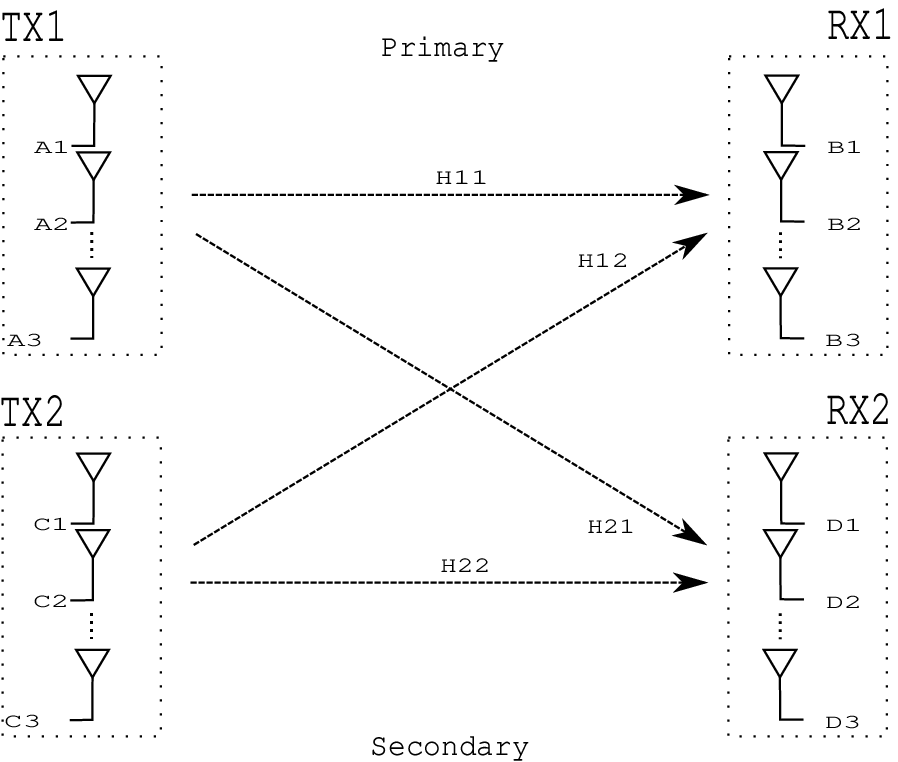
Refer to caption — Figure 1: Two-user MIMO interference channel.

From Spectrum Pooling to Space Pooling: Opportunistic Interference Alignment in MIMO Cognitive Networks

Abstract

I Introduction

II System Model

III Interference Alignment Strategy

III-A Primary Link Performance

Theorem 1

III-B Transmit Opportunities

Definition 2 (Transmit Opportunities)

III-C Pre-processing Matrix

Definition 3 (IA condition)

Lemma 1 (Pre-processing matrix 𝐕2\mathbf{V}_{2})

Proof:

III-D Post-processing Matrix

III-E Power Allocation Matrix Optimization

III-E1 Uniform Power Allocation

III-E2 Optimal Power Allocation

IV Asymptotic Performance of the Secondary link

Definition 4 (Regime of Large Numbers of Antennas)

IV-A Asymptotic Number of Transmit Opportunities

IV-B Asymptotic Transmission Rate of the Opportunistic Link

Proposition 5 (Asymptotic Transmission Rate)

Proof:

V Numerical Results

V-A The Number SS of Transmit Opportunities

V-B Comparison between OIA and ZFBF

V-B1 Case Nt>NrN_{t}>N_{r}

V-B2 Case Nt⩽NrN_{t}\leqslant N_{r}

V-C Asymptotic Transmission Rate

VI Conclusions

Appendix A Proof of Lemma 1

Proof:

Appendix B Definitions

Definition 6

Appendix C Proof of Proposition 5

References

Lemma 1 (Pre-processing matrix $\mathbf{V}_{2}$ )

V-A The Number $S$ of Transmit Opportunities

V-B1 Case $N_{t}>N_{r}$

V-B2 Case $N_{t}\leqslant N_{r}$