Poisson-Boltzmann cell model for heterogeneously charged colloids
Abstract
We introduce the Poisson-Boltzmann cell model for spherical colloidal particles with a heterogeneous surface charge distribution. This model is obtained by generalizing existing cell models for mixtures of homogeneously charged colloidal spheres. Our new model has similar features as Onsager’s second-virial theory for liquid crystals, but it predicts no orientational ordering if there is no positional ordering. This implies that all phases of heterogeneously charged colloids that are liquid-like with respect to translational degrees of freedom are also isotropic with respect to particle orientation.
I Introduction
Already a long time ago Marcus [1], Ohtsuki et al. [2] and Alexander et al. [3] realized that the cell model approach of Wigner and Seitz [4] to calculate the properties of electrons in solids can also be applied to colloidal matter. In this case there are no quantum effects, and in stead of a wave function one calculates the ion-distributions around charged colloidal particles dispersed in a liquid medium. In the simplest case, the colloidal dispersion consists of one colloidal species immersed in a 1:1 electrolyte solution. The colloidal particles are homogeneously charged and have a spherical shape. Additionally, the simplification of taking a spherical Wigner-Seitz cell—instead of space filling—is justified in fluid phases with no broken translational symmetry.
A number of extensions has been made to this basic cell model. There is the eccentric Poisson-Boltzmann cell model [2, 5], and the heterogeneous—or polydisperse—cell model [6, 7], to describe mixtures. Additionally, the cell model has been extended by applying cylindrical Wigner-Seitz cells for the description of disc-shaped and rodlike particles [8, 9]. In the present paper, we make an extension towards particles with an heterogeneous surface charge distribution, such as patterned colloids [10] or Janus particles [11]. Janus particles are characterized by two distinct regions of surface area. Each of these “faces” has a different chemical composition, which can create spontaneous aggregation [12]. Our aim is towards a description of self-organization of these particles from single-particle properties. The cell model can be a powerful tool, giving a simple description of these complex systems. From this description, a number of thermodynamic quantities can be derived such as free energy, and osmotic pressure.
We investigate how surface charge heterogeneity influences the distribution of particle orientations in the case of a homogeneous positional distribution. This case can be considered as a simplified description of a fluid of these particles, but also as an over-simplified description of a solid. Since the particle interactions are implemented through the boundary conditions of the Wigner-Seitz cell, one can choose to neglect the correlations between the orientational and positional ordering. The basis of our model is the generalization of the Poisson-Boltzmann cell model by Biesheuvel et al. [6] considering mixtures, together with the insight of Onsager [13] that a distribution of orientations can be considered in the same way as mixtures. In principle, this model can be used to predict the phase behavior of a large class of colloidal and nanoparticles, because an anisotropic (as well as spherical) particle shape can be treated. However, here we restrict ourselves to a system of spherical colloidal particles.

II The cell model for mixtures
We start by giving the prerequisites for the ordinary spherically symmetric cell model (see Fig. 1). In this simple case, we consider a system of identical, spherically symmetric colloidal particles in a volume . These particles have radius and a surface charge , where is the elementary charge. The system is presumed to be in osmotic contact with a reservoir of monovalent cations and anions at total concentration , with charge . Both the particle and the surrounding medium are considered to be dielectric media, where and are the dielectric constants of the particle and the solvent, respectively.
Within Poisson-Boltzmann theory, one relates the denisty profiles of the ions to the electrostatic potential in a fixed configuration of the colloidal particles. This complicated nonlinear -body problem can be simplified considerably by considering a single colloidal particle in the center of a Wigner-Seitz cell, surrounded by the ions. This cell is assumed to have a spherical shape (of radius ) instead of space filling. The volume of the cell is fixed by the available volume per particle,
| (1) |
We treat the ions in a mean field description, such that we obtain the Poisson-Boltzmann (PB) equation
| (2) |
where is the Debye screening length, and is the dimensionless electrostatic potential, where . This second-order nonlinear partial differential equation describes the electrostatic effects of the ions in the cell volume surrounding the colloidal particle. The boundary conditions are determined by the charge on the particle and the cell electroneutrality. The first boundary condition is given by
| (3) |
| (4) |
which fixes the electric field at the particle surface. In Eq. (4), is the number of elementary charges on the particle surface. Because of the homogeneous surface charge distribution, there is no electric field inside the particle. This reduces boundary condition (4) to
| (5) |
where is the Bjerrum length. The second boundary condition fixes the electric field at the cell boundary, according to Gauss’ law
| (6) |
The PB-equation (2) together with the boundary conditions (5) and (6) form a closed set and describe the basic Poisson-Boltzmann cell model as studied for example in Refs. [3, 14, 15].
Now we discuss the case of a mixture of equally sized, homogeneously charged colloidal species with surface charge . Again, the particles have radius , and are positioned in the center of a spherical Wigner-Seitz cell of radius . The PB-equation (2) is solved separately for each colloidal species , and the notion of electroneutrality is applied to the system as a whole [6]. Each solution is determined by the surface charge density on the corresponding colloidal species
| (7) |
Given that the cells of each pair of species are considered to be neighboring, it is natural to impose a common boundary value for the potential on every cell surface. This value is by definition equal to the average value of the electrostatic potential at the cell boundary for different species. Hence, we have
| (8) |
where is the molar fraction of species , such that
| (9) |
The boundary value is fixed by setting the average value of the charge contained in the cells for different species to zero. According to Gauss’ law, this is achieved by imposing
| (10) |
The PB-equation (2) applied to each species together with the boundary conditions (7), (8), and (10) again form a closed set.
In principle, one could allow for a different cell radius for each colloidal species. In this case, a factor must be included in the summation of Eq. (10). One subsequently imposes a set of physically motivated conditions on these radii. These conditions must comply with the fact that the average cell volume of the system is given by
| (11) |
In the case of mixtures where the charge of all species has the same sign, one can fix each by imposing the condition that the electric field must vanish at the cell boundary of each species [7]. For reasons of simplicity, however, we will not use such an extension. Hence, in this paper, the cell radius is given by a single value .
III An extension towards heterogeneous charge distributions
We now consider a system of spherical colloidal particles that are not homogeneously charged, such as Janus particles [11]. Again, the system consists of identical spherical particles of radius in a volume . We apply the same Poisson-Boltzmann theory, such that the electrostatic potential obeys the PB-equation (2). As before, we fix the position of each particle at the center of a spherical Wigner-Seitz cell of radius , and the PB-equation must be solved for each “species”. However, in this case we replace the species index by an orientation , and each solution is denoted by . In the spirit of Onsager, we can view such an orientational distribution as a mixture where the different particle species have a distinct charge distribution.
In this paper, we focus on charge distributions that are cylindrically symmetric with respect to the particle orientation . This charge distribution gives us the boundary condition on the particle surface at each position
| (12) |
| (13) |
where is the surface charge density (in units of ) that belongs to a particle with an orientation , and is the relative dielectric constant of the particle with respect to the surrounding solvent. The labels “in” and “out” denote the solutions inside the colloidal particle, and outside the particle, respectively.

Next, we must supply a generalized version of the boundary conditions on the cell surface given in Eqs. (8) and (10). The following approach is illustrated by Fig. 2, which shows the directionality that must be included in the appropriate boundary conditions. First, the concept of a fixed cell surface potential is applied to include different positions on the cell surface. Similar to the cell model for mixtures, the value of this potential is defined as the average value of the electrostatic potential at the cell boundary for different orientations. However, the average value is taken at the position of opposite orientation
| (14) |
where instead of a summation over species weighted by the molar fractions , we have an integral over particle orientations weighted by the orientational distribution function (ODF)
| (15) |
This distribution is normalized such that
| (16) |
The definition of the cell surface potential in Eq. (14) is such that it is always an even function
| (17) |
Finally, we have to impose a boundary condition that fixes this cell surface potential. However, if we only impose global electroneutrality on the system, we obtain a boundary condition that is too general for a solution that is not spherically symmetric. It would ensure that the average value (over all “species”) of the charge contained in each Wigner-Seitz cell vanishes. By applying Gauss’ law, we see that this condition is satisfied by setting the average value of the electric field integrated over the surface to zero
| (18) |
Interestingly, this fixes only the isotropic contribution to the cell surface potential. Therefore, we impose an additional condition that is based on the concept of continuity of the electric field flux from one cell to another. The difference between the outward flux at the cell boundary and the average inward flux of neighboring cells is represented by
| (19) |
This quantity is averaged over all particle orientations, and set to zero, in order to insure global electric field flux conservation
| (20) |
which is equivalent to imposing
| (21) |
This condition does fix the cell surface potential, and it defines an average boundary value of the radial derivative such that it is an odd function of .
IV Special limiting cases: perfectly isotropic and perfectly aligned
In this section, we apply specific choices for the ODF. In turn, these choices yield a specific form for the boundary conditions (14) and (21). The resulting models are less intricate than the full model we presented in the previous section. Also, these models yield boundary conditions that one would expect from a naive description of such systems.
Let us take a look at the model that our boundary conditions yields when we implement specific ODFs. First, we consider a perfectly isotropic orientational distribution
| (22) |
Since in such a system there is no preferential direction, we argue that all solutions—for different particle orientations—are equivalent. Consequently, the cell surface potential is independent of the position on the cell surface
| (23) |
This result is in accordance with the notion that in the isotropic case the average over all particle orientations (15) is equal to the average over all orientations of the position on the cell surface, and that this average no longer depends on either orientation. Therefore, the boundary condition (21) is equivalent to the condition that each cell is electroneutral
| (24) |
V Application to linearized Poisson-Boltzmann theory
To solve the full nonlinear problem is possible numerically, but it turns out to be very involved [16]. Therefore, we restrict ourselves to the linearized version of Poisson-Boltzmann theory. In this case, the nonlinear right hand side of the PB-equation is linearized around a certain value. We denote it by , such that the linearized Poisson-Boltzmann (LPB) equation is given by
| (29) |
In some cases, the value for is chosen to be zero. This choice is meaningful if the concentration of colloids, as well as the total surface charge density, is low. Alternatively, its value can be set to the isotropically averaged value of the potential at the cell boundary. This choice is particularly useful when one has the boundary values of the potential and the electric field from numerical calculations of the nonlinear PB-equation [16]. These can be used to fit renormalized charge distributions on the particle surface using the expression in Eq. (33). Lastly, one can apply the Donnan potential as the value around which to perform the linearization. This value requires no other input than the colloid concentration, its particle radius, its total surface charge, and the reservoir salt concentration [14]. In this paper, we leave unspecified.
Inside the colloidal particle still satisfies the Laplace equation. It is natural in this case to expand both the inner and the outer solution in spherical harmonics. This leads to two sets of coefficients which have to be matched at the particle surface. Inside the particle
| (30) |
whereas in the cell interior
| (31) |
where , and and are the modified spherical Bessel functions of order of the first and second kind, respectively. The boundary condition on the particle surface are given by Eqs. (12) and (13), where we decompose the charge distribution as
| (32) |
Next, we impose the boundary conditions at the cell surface, which are given in Eqs. (14) and (21). Together, this yields the general solution for the dimensionless electrostatic potential in the cell interior
| (33) |
where
| (34) | ||||
| (35) |
The details of the derivation of the expression in Eq. (33) can be found in appendix A. Note that the first sum (over all ) does not depend on the ODF, whereas it does depend on the particle orientation . This contribution to the potential is purely due to the particle at the center of the cell, and it vanishes at the cell boundary. Conversely, the second sum (over even ) does not depend on the particle orientation, whereas it does depend on the ODF. This means that it describes the effect of all the surrounding particles. Moreover, it vanishes in the limit of infinite dilution ().
The thermodynamic potential for the ion distribution in a single cell is given by [14]
| (36) |
where the the label “out” at the integral symbol denotes integration over the cell interior (i.e., the domain of ), and is the reservoir salt concentration (such that ). We cannot evaluate this expression analytically. Therefore, we linearize it around to find
| (37) |
where
| (38) | ||||
| (39) | ||||
| (40) |
It turns out that depends on the particle orientation and the ODF, whereas the other two terms depend on neither. The expression we obtain can be derived through another route, by expanding the original non-linear functional of the ion profiles up to second order with respect to a density . Minimizing this functional with respect to the ion profiles yields the LPB-equation (29), and the accompanying expressions for the ion profiles . Substitution of this expression into the functional yields Eq. (37).
VI Onsager-like second-order density functional theory
We approximate the total free energy (per colloidal particle) of the system by averaging over all particle orientations. Also, we add an entropic contribution, which is analogous to mixing entropy
| (41) |
We neglect the translational entropic contributions of the colloidal particles, because we are only interested in the effects of charge anisotropy and orientational distribution. Using the identity
| (42) |
which can be easily derived from Eq. (32) using the addition theorem, we derive the following expression for the free energy
| (43) |
where
| (44) |
and
| (45) |
Note that the second term of vanishes if one chooses the Donnan potential for the value of . Also, the entire contribution from vanishes upon taking the functional derivative with respect to .
The structure of the free energy functional (43) is remarkably similar to that of Onsager’s second-virial theory for hard rods [13]. In the case of spherocylinders, the kernel stems from hard-core interactions, and it is equal to the product of the rod density and the orientation dependent excluded volume of one rod in the vicinity of another,
| (46) |
where is the rod length, is the rod diameter. The angle between the two rod orientations is defined by . Onsager’s second-virial theory predicts the existence of an isotropic–nematic transition, caused by the competition between orientational and translational entropy. In the low-density isotropic phase, the “mixing” term is minimized by an isotropic orientational distribution, whereas the contribution due to the average excluded volume is minimized in the high-density nematic phase. This transition only occurs if the length-to-diameter is large, such that the kernel is sufficiently anisotropic, with a maximum at . In the limit , the description by Onsager is quantitative.

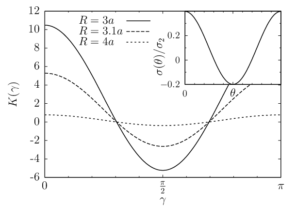
In the present case, the kernel stems from anisotropic electrostatic interactions, and we will investigate if these can give rise to such a symmetry-breaking transition. In both cases, the kernel is rotationally invariant, i.e., it only depends on the mutual relative orientation of the unit vectors and —through the dot product . Figure 3 shows the values of the kernel for two distinct surface charge distributions . The angle between the axis of symmetry and the position vector on the surface is defined by . The top graph shows a highly peaked distribution around and in the inset. However, the kernel is much less anisotropic in this case. The lower graph has a purely quadrupolar distribution, which reflects in the fact that the kernel the same orientational dependence. In both cases, the kernel has a minimum at . Consequently, we expect no isotropic–nematic transition. In the next section, we prove that this conclusion holds for any choice of parameters.
VII Bifurcation theory
The ODF that minimizes the free energy (43) obeys the Euler-Lagrange equation
| (47) |
where we introduced the Lagrange multiplier to ensure the normalization of given by Eq. (16). The Euler-Lagrange equation can be rewritten in a form that always satisfies this normalization
| (48) |
One easily checks that is a solution of Eq. (48), describing the perfectly isotropic phase. Due to its nonlinear character, one can expect additional (anisotropic) solutions to this equation. Finding explicit expressions for these solutions, however, is difficult, although good insight can be obtained form a bifurcation analysis. The goal of this analysis is to determine if—and for what parameters—an instability can be found in the reference solution with respect to a perturbation.
We choose the isotropic ODF (22) as a reference, and expand around this solution by writing , with a small deviation. Following the same scheme as Kayser and Raveché [17] applied to Onsager’s model of hard rods—which was extended by Mulder [18]—we find the bifurcation equation
| (49) |
This is an eigenvalue equation, for which a non-trivial solution exists if the integral operator has eigenvalues . The parameter value for which this occurs is called the bifurcation point, where an anisotropic solution branches off from the (isotropic) reference solution. The solution to the bifurcation equation (49) can be given in terms of eigenfunctions of . On the basis of rotational-symmetry arguments, we find that these eigenfunctions are the Legendre polynomials of the dot product of the orientation with respect to an arbitrary direction,
| (50) |
where the eigenvalues follow from Eq. (45),
| (51) |
The bifurcation point is determined by . However, all coefficients are positive. Therefore the bifurcation equation (49) has no solution, and there is no bifurcation point. The understanding of the origin of this property of the coefficients lies in the fact that both and approach their minimum in the limit . Moreover, these limits are non-negative, since
| (52) |
| (53) |
This result shows that the breaking of orientational symmetry cannot be captured in this simple version of Poisson-Boltzmann cell theory. Additionally, it strongly suggests that there must be positional order before there can be orientational ordering in suspensions of Janus or other patchy particles. In other words, the transition from an isotropic state to a fully ordered crystal phase—if it exists—will be intermitted by a plastic crystal phase. Our simple cell model does not take into account the positional correlations of the plastic crystal phase, due to the mean-field nature of the applied boundary conditions at the cell surface.
VIII Conclusion and outlook
We developed a simple cell model in the context of Poisson-Boltzmann theory for heterogeneously charged colloidal spheres. The boundary conditions—on the colloid surface as well as on the Wigner-Seitz cell surface—depend on the charge heterogeneity and the orientational distribution of the colloidal particles. Within a linear approximation to Poisson-Boltzmann theory, these boundary conditions give rise to a free-energy functional of the orientational distribution function that is very similar to the one used in Onsager’s second-order virial approximation in the description of the isotropic–nematic transition of hard rods [13]. The present description, however, does not give rise to orientational ordering. Since our model treats the position of the colloids in a mean field description—and since we do expect some degree of orientational ordering at sufficiently high particle density—this result suggests that orientational ordering requires the existence of positional ordering. The present theory predicts no orientational ordering in fluids of these particles, i.e., no liquid crystal phases. On the other hand, this effect can also be attributed to an oversimplification of our description. In that sense, the orientational ordering could be the result of particle pair correlations which are not included in our model.
Therefore, one could consider to expand the class of Poisson-Boltzmann cell models even further. Conceivably, a method can be devised to include correlations of particle positions through the electrostatic boundary conditions. More specifically, one can choose a different approach to the way that the surface potential is determined. In the present models, this potential is independent of the colloidal species to which the cell belongs. Also, each colloidal species has an equivalent weight—equal to its molar fraction—in the average of the potential and electric field flux at the cell boundary. This property is due to the mean field description which is used. Also inherent to this description is the assumption that the surrounding of a particle at the cell boundary is independent from the species it belongs to—or equivalently, its orientation. However, if this restriction is lifted, one may include the fact that the surroundings do depend on this property through the pair distribution function.
The nature of these correlations can be related in a simple way to systems of oppositely charged colloidal particles [19, 20]. The number of bonds between oppositely charged particles in these systems depends on the colloid density. Also, for the dense liquid phase—coexisting with a dilute vapor phase provided the Debye screening length is large enough—the pair distribution function shows that a colloidal particle is surrounded by different layers of colloidal species with alternating signs of charge [19]. The first surrounding layer has an opposite charge with respect to the particle in the origin; the following layer is like-charged, and so on. These systems also display multiple crystal structures, which have different coordination number. The same notion can be subsequently applied to particles of different orientations to include orientational pair correlations in the cell model. This paves the way to a description of orientationally ordered phases. Additionally, a jellium approximation can be applied in the same way it is applied to monodisperse systems of homogeneously charged colloidal spheres and rods [21, 22]. In this description, there is no need for a certain cell shape and volume. Moreover, the jellium model has a natural way to include particle pair correlations [23, 24]. Finally, there is an opportunity to apply the Poisson-Boltzmann cell model to non-spherical cells [25]. The boundary conditions can be imposed in the same way as in this paper. However, this complicates the expression of the appropriate boundary conditions, since a non-spherical shape will couple different spherical harmonic modes. The shape of these cells must be controlled by additional constraints, such as the minimization of free energy. Also, the choice of shapes must be motivated by physical arguments. We leave these options for future studies.
Appendix A Derivation of the electrostatic potential
Inside the colloidal particle satisfies the Laplace equation, whereas in the cell interior it satisfies the LPB-equation. Therefore, we have to match two general solutions, using the boundary conditions on the particle surface. We do this by expanding both solutions in spherical harmonics. These expressions are given in Eqs. (30) and (31). We apply the boundary condition on the particle surface, given by Eqs. (12) and (13). To this end, we expand the surface charge distribution in spherical harmonics, using Eq. (32) and the addition theorem,
| (54) |
The arguments and of the spherical harmonic function should be interpreted as the pair of spherical angles of this orientation with respect to the reference frame. Consequently, from the boundary conditions (12) and (13), we obtain the following condition on the coefficients of ,
| (55) |
Next, we apply the boundary conditions at the cell surface given in Eqs. (14) and (21). This yields a linear system of equations, which can be solved analytically. However, we can choose to split the solution into two contributions. The first contribution then satisfies the boundary conditions on the particle surface—given by Eq. (55)—as well as the condition that the potential vanishes at the cell boundary. This is already the relevant boundary condition for all odd contributions to , whereas a second contribution must be added later to the even contributions in order to satisfy the full set of boundary conditions. The coefficients that belong to the first contribution will be denoted by and . First, we impose the vanishing potential at the cell boundary by
| (56) |
Together with Eq. (55), this yields
| (57) | ||||
| (58) |
where is defined in Eq. (34). The orientational dependence of this first contribution is such that it—and therefore all odd contributions—only depends on the angle between and ,
| (59) |
As previously mentioned, a second contribution must be added to the coefficients of the even contributions. With this contribution included, the solution satisfies the full set of boundary conditions on the cell surface given in Eqs. (14) and (21). We denote the coefficients of this secondary contribution by and . Also, we show that these do not dependent on the particle orientation, because the two distinct boundary conditions that govern them do not. First, the boundary condition (55) is already satisfied by the coefficients and . Therefore,
| (60) |
Second, the boundary condition (14) imposes a value on the coefficients that only depends on the value of the potential at the cell surface, which is necessarily independent of the orientation . Hence,
| (61) |
where is defined by
| (62) |
Together, these conditions yield
| (63) | ||||
| (64) |
Finally, the boundary condition (21) imposes a vanishing value of the weighted average of the even contributions to the electric field flux at the cell boundary. This condition can be expressed in terms of a relation between the coefficients , , , and . By substituting the values given in Eqs. (57) and (58), we arrive at
| (65) |
where we used
| (66) |
which can be derived from standard identities for the modified spherical Bessel functions. The conditions in Eqs. (60) and (65) are sufficient to derive similar expressions for and . However, the construction we use to derive the solution to the even contributions enables us to show that the cell surface potential has the same symmetry properties as the ODF (in addition to the fact that it is composed purely of even contributions),
| (67) |
where is defined in Eq. (35). With this we readily obtain the even contributions
| (68) |
and we obtain the general solution for the dimensionless electrostatic potential in the cell interior given in Eq. (33).
References
- [1] R. A. Marcus, J. Chem. Phys. 23, 1057 (1955).
- [2] T. Ohtsuki, S. Mitaku, and K. Okano, Jpn. J. Appl. Phys. 17, 627 (1978).
- [3] S. Alexander, P. M. Chaikin, P. Grant, G. J. Morales, P. Pincus, and D. Hone, J. Chem. Phys. 80, 5776 (1984).
- [4] E. Wigner and F. Seitz, Phys. Rev. 43, 804 (1933).
- [5] H. H. von Grünberg and L. Belloni, Phys. Rev. E 62, 2493 (2000).
- [6] P. M. Biesheuvel, S. Lindhoud, R. de Vries, and M. A. Cohen Stuart, Langmuir 22, 1291 (2006).
- [7] A. Torres, G. Téllez, and R. van Roij, J. Chem. Phys. 128, 154906 (2008).
- [8] J.-P. Hansen and E. Trizac, Physica A 235, 257 (1997).
- [9] L. Bocquet, E. Trizac, and M. Aubouy, J. Chem. Phys. 117, 8138 (2002).
- [10] S. C. Glotzer and M. J. Solomon, Nature Mater. 6, 557 (2007).
- [11] A. Walther and A. H. E. Müller, Soft Matter 4, 663 (2008).
- [12] L. Hong, A. Cacciuto, E. Luijten, and S. Granick, Nano Lett. 6, 2510 (2006).
- [13] L. Onsager, Ann. N.Y. Acad. Sci. 51, 627 (1949).
- [14] H. H. von Grünberg, R. van Roij, and G. Klein, Europhys. Lett. 55, 580 (2001).
- [15] E. Trizac, L. Bocquet, M. Aubouy, and H.-H. von Grünberg, Langmuir 19, 4027 (2003).
- [16] N. Boon, E. Carvajal Gallardo, S. Zhang, E. Eggen, M. Dijkstra, and R. van Roij (2009), arXiv:0904.2532.
- [17] R. F. Kayser, Jr. and H. J. Raveché, Phys. Rev. A 17, 2067 (1978).
- [18] B. M. Mulder, Phys. Rev. A 39, 360 (1987).
- [19] J. B. Caballero, A. M. Puertasa, A. Fernández-Barbero, and F. J. de las Nieves, J. Chem. Phys. 121, 2428 (2004).
- [20] M. E. Leunissen, C. G. Christova, A.-P. Hynninen, C. P. Royall, A. I. Campbell, A. Imhof, M. Dijkstra, R. van Roij, and A. van Blaaderen, Nature 437, 235 (2005).
- [21] E. Trizac and Y. Levin, Phys. Rev. E 69, 031403 (2004).
- [22] S. Pianegonda, E. Trizac, and Y. Levin, J. Chem. Phys. 126, 014702 (2007).
- [23] R. Castañeda-Priego, L. F. Rojas-Ochoa, V. Lobaskin, and J. C. Mixteco-Sánchez, Phys. Rev. E 74, 051408 (2006).
- [24] T. Colla, Y. Levin, and E. Trizac (2009), submitted; arXiv:0905.1620.
- [25] H. Graf, H. Löwen, and M. Schmidt, Prog. Coll. Poly. Sci. 104, 177 (1997).