跳到论文正文
W Papers独立论文阅读器 arXiv:0907.1061 论文正文 计算阅读时间 · 0%
引用这篇论文根据当前论文元数据生成,正式投稿前建议核对。


License: arXiv.org perpetual non-exclusive license
arXiv:0907.1061v6 [cs.IT] 10 Dec 2013

Boolean Compressed Sensing and
Noisy Group TestingThanks: This research was partially supported by NSF CAREER award ECS 0449194 and NSF Grant 0932114, by the U.S. Department of Homeland Security under Award Number 2008-ST-061-ED0001

George Kamal Atia†    Venkatesh Saligrama‡ ††thanks: † G. Atia is with the Coordinated Science Laboratory (CSL) at the Department of Electrical and Computer Engineering at the University of Illinois at Urbana-Champaign. ‡ V. Saligrama is with the Information Systems and Sciences Laboratory (ISS) at the Department of Electrical and Computer Engineering at Boston University. This work was presented in part at the Allerton Conference on Communication, Control, and Computing, Monticello IL, in September 2009 [1]. The authors can be reached at: atia1@illinois.edu, srv@bu.edu.
Abstract

The fundamental task of group testing is to recover a small distinguished subset of items from a large population while efficiently reducing the total number of tests (measurements). The key contribution of this paper is in adopting a new information-theoretic perspective on group testing problems. We formulate the group testing problem as a channel coding/decoding problem and derive a single-letter characterization for the total number of tests used to identify the defective set. Although the focus of this paper is primarily on group testing, our main result is generally applicable to other compressive sensing models.

The single letter characterization is shown to be order-wise tight for many interesting noisy group testing scenarios. Specifically, we consider an additive Bernoulli(qq) noise model where we show that, for NN items and KK defectives, the number of tests TT is O⁡(K​log⁡N1−q)O\left(\frac{K\log N}{1-q}\right) for arbitrarily small average error probability and O⁡(K2​log⁡N1−q)O\left(\frac{K^{2}\log N}{1-q}\right) for a worst case error criterion. We also consider dilution effects whereby a defective item in a positive pool might get diluted with probability uu and potentially missed. In this case, it is shown that TT is O⁡(K​log⁡N(1−u)2)O\left(\frac{K\log N}{(1-u)^{2}}\right) and O⁡(K2​log⁡N(1−u)2)O\left(\frac{K^{2}\log N}{(1-u)^{2}}\right) for the average and the worst case error criteria, respectively. Furthermore, our bounds allow us to verify existing known bounds for noiseless group testing including the deterministic noise-free case and approximate reconstruction with bounded distortion. Our proof of achievability is based on random coding and the analysis of a Maximum Likelihood Detector, and our information theoretic lower bound is based on Fano’s inequality.

Index Terms: 
Compressed sensing, group testing, ML decoding, sparse models.

I Introduction

Group testing has been effectively used in numerous applications. It was originally proposed during World War II to reduce the total number of blood tests required to detect soldiers with Syphilis [2, 3]. Instead of conducting a separate blood test for each and every soldier, the idea was to pool blood samples from many soldiers and test them simultaneously. Group testing has been used in general in biology for screening libraries of DNA clones (strings of DNA sequence) of the human genome and for screening blood for diseases. Other applications include quality control for detecting defective parts in production lines, data forensics to test collections of documents by applying one-way hash functions, computer fault diagnosis, and contention algorithms in multiple access communications. Recently, group testing methods have also been applied to spectrum enforcement in cognitive radios  [4, 5].

In the basic group testing problem [2], we are given a population of NN items. Among them, at most KK items, also called defectives, are of interest. The set of defectives is denoted by 𝒢\cal G. Associated with the group testing problem is a binary matrix 𝑿X known as the measurement matrix. This matrix defines the assignment of each of the items to different pools or collections. The (i,j)(i,j) entry is 11 if the ii-th item is contained in the jj-th pool and 00 otherwise. A test conducted on the pool is positive if there is at least one item belonging to the pool which is also an element of 𝒢\cal G, and is negative otherwise. A measurement matrix for a non-adaptive group testing algorithm is a N×TN\times T matrix where the TT columns correspond to pools of items and NN is the number of items. Each item is associated with a row codeword of length TT. If KK items are defective, then the TT tests are a boolean sum of KK rows of the measurement matrix. The goal is to construct a pooling design to recover the defective set while reducing the required number of tests. Group testing is related in spirit to compressed sensing (CS). In CS we are given an N-dimensional sparse signal with support size KK. Random projections of the sparse signal are obtained. The goal is to identify the support set while minimizing the number of projections. In this sense, group testing can be viewed as a boolean version of CS where we apply a measurement matrix to a sparse vector corresponding to the defective set with the goal of reconstructing the support, i.e. identify the defective items. The main distinction is that in group testing the test matrix used to collect the measurements is binary, so is the sparse vector, and the arithmetic is boolean. Multiplication of 00s and 11s is the logical AND (coincides with usual multiplication) but addition is replaced by the logical OR.

While the degradation of CS with noise has been characterized (see  [6, 7, 8, 9, 10, 11, 12] and references therein), the noisy group testing problem, the main focus of this paper, has been mostly unexplored. Our attention in this paper is on the so called non-adaptive testing problem [2], where the measurement matrix is formed prior to performing the tests.

A significant part of the existing research on group testing is focused on combinatorial pool design (i.e. construction of measurement matrices) to guarantee the detection of the items of interest using a small number of tests. Two types of matrix constructions have been considered. Disjunct matrices [2] satisfy the so called covering property11 1 We say that a row xx is covered by a row yy iff x∨y=yx\vee y=y.. In the context of group testing this property implies that a test pattern obtained by taking any KK rows of the measurement matrix does not cover any other boolean sum of KK or smaller number of rows22 2 In the combinatorial pool design literature, the roles of rows and columns are interchanged. In other words, the measurement matrix is 𝑿T\text{\boldmath{$X$}}^{T}, i.e., the transpose of our matrix 𝑿X. What motivates our choice is consistency with the standard information theoretic convention for codewords being rows of a codebook.. Equivalently, for any K+1K+1 rows, there always exists a column with 11 in a row and 00s in the other KK rows. Matrices that satisfy this property are often referred to as superimposed codes and combinatorial constructions were extensively developed by  [13, 14, 15]. Superimposed codes are not only desirable because they ensure identifiability but they also lead to efficient decoding. Separability [2] is a weaker notion that is also often employed. A separable matrix ensures that the boolean sums of KK rows are all distinct, which ensures identifiability. Uniquely decipherable codes [14, 13] are codes that guarantee that every boolean sum of KK or smaller number of rows are distinct. Recently, it has been shown [16] that all of these notions are equivalent up to a scaling factor on the number of tests TT.

A different approach to group testing based on probabilistic method has also been advocated by several researchers [17, 18, 19, 20, 21]. Dyachkov and Rykov [17], Du and Hwang [22], and Ruszinko [18] developed upper and lower bounds on the number of rows TT for a matrix to be KK-disjunct (bound on length of superimposed codes). Random designs were used to compute upper bounds on the lengths of superimposed codes by investigating when randomly generated matrices have the desired covering/separability properties. They showed that for N→∞N\rightarrow\infty and K→∞K\rightarrow\infty, the number of tests TT must scale as T=O⁡(K2​log⁡Nlog⁡K)T=O\left(\frac{K^{2}\log N}{\log K}\right) for exact reconstruction with worst-case input. Sebo [19] investigated average error probabilities and showed that for an arbitrarily small error probability, a randomly generated matrix will be KK-disjunct if T=O⁡(K​log⁡N)T=O(K\log N) as N→∞N\rightarrow\infty. Recently Berger et al. [20] proved upper and lower bounds on the number of tests for two-stage disjunctive testing. Approximate reconstruction [21], whereby a fraction α\alpha of the defective items are allowed to be in error, has been described. Again the number of tests here has been shown to scale as T=O⁡(K​log⁡N)T=O(K\log N) as N→∞N\rightarrow\infty.

While these approaches have generally characterized fundamental tradeoffs for noiseless group testing, the noisy counterpart of group testing has been largely unexplored. In this paper we present a novel information theoretic approach to group testing problems. The common approach to previous related work was to prove bounds on the size of randomly generated matrices to exhibit the aforementioned separability and covering properties. In contrast, we formulate the problem as a detection problem and establish its connection to Shannon coding theory  [23]. While there exists a one-to-one mapping between both formulations, the new perspective allows us to easily obtain results for a wide range of models including noisy versions of group testing. Our approach, which is fairly general, is to map the group testing problem to a corresponding channel model which allows the computation of simple mutual information expressions to derive achievable bounds on the required number of tests. Very recently, it came to our attention that related work that uses a similar information theoretic approach for noisy group testing has been independently explored in the Russian literature [24, 25, 26, 27, 28]. One main difference between those approaches and our approach is that, in the earlier work, the number of defective items, KK, is held fixed while the number of items, NN, approaches infinity. Consequently, those bounds suggest that the number of tests must scale poly-logarithmically in NN regardless of KK for error probability to approach zero. In contrast we consider the fully high-dimensional setting wherein both the number of defectives as well as the number of items can approach infinity. This implies that our bounds not only depend on NN but also explicitly on the number of defectives. In addition our approach also has other advantages, including:

  • •

    Mutual information characterization: Our main result is a simple single letter characterization providing order-wise tight necessary and sufficient conditions on the total number of tests.

  • •

    Characterization for new group testing problems: This result allows us to verify existing bounds for some of the known scenarios and extend the analysis to many new interesting setups including noisy versions of group testing. We present bounds that explicitly characterizes the required number of tests in terms of the number of defectives and the number of items. Our analysis includes the fully high-dimensional case where both the number of defectives and the number of items approach infinity.

  • •

    Extensions to sparse models: Although the focus of this paper is on the Boolean case, the main result and the methods that we develop in this paper are more generally applicable to Compressed Sensing models and not just to group testing. The results extend beyond binary variables and Boolean arithmetic to the general problem of support recovery with arbitrary discrete alphabet [29]. Consequently, some of the information theoretic Compressed Sensing results [30] can also be recovered using the mutual information expressions derived herein.

One major contribution of this paper is to develop tools to analyze long standing noisy versions of the group testing problem. In particular we consider two models: The dilution model and the additive model.

  • •

    Additive model: False alarms could arise from errors in some of the screening tests. This arises when some tests are erroneously positive.

  • •

    Dilution model: Even though a positive item is contained in a given pool, the test’s outcome could be negative if the defective item gets diluted for that specific test. For example, in blood testing the positive sample might get diluted in one or more tests leading to potential misses of infected blood samples. To account for such a case we analyze the group testing problem where some of the positive entries get flipped into zeros with a given probability uu.

We also consider the case of partial reconstruction where we only aim for approximate recovery of the defective set. An error occurs only if the number of missed defectives is greater than a fraction α\alpha of the total KK defectives.

Model TT (average PeP_{e} criterion) TT (max⁡Pe\max P_{e} criterion)
Noise-free O⁡(K​log⁡N)O(K\log N) O⁡(K2​log⁡N)O(K^{2}\log N)
Partial reconstruction O⁡(K​log⁡N)O(K\log N) O⁡(K​log⁡N)O(K\log N)
Noisy with additive noise O⁡(K​log⁡N1−q)O\left(\frac{K\log N}{1-q}\right) O⁡(K2​log⁡N1−q)O\left(\frac{K^{2}\log N}{1-q}\right)
Noisy with dilution O⁡(K​log⁡N(1−u)2)O\left(\frac{K\log N}{(1-u)^{2}}\right) O⁡(K2​log⁡N(1−u)2)O\left(\frac{K^{2}\log N}{(1-u)^{2}}\right)
TABLE I: This table summarizes the scaling results for the various models considered in the paper which hold asymptotically for N→∞N\rightarrow\infty. In particular, it shows the required number of tests TT as a function of the size of the defective set KK, the total number of items NN, and the model parameters for the noiseless, additive noise, and dilution models for both the average error and worst-case error criteria. The probability qq is the parameter of the Bernoulli(qq) additive noise, and uu is the dilution probability for the dilution model.

Table I summarizes the scaling results we obtained for the various models considered in the paper for the average error and worst case error criteria.

The rest of the paper is organized as follows. Section II describes the problem setup. The main achievable result mapping the problem to mutual information expression is provided in Section III. In Section IV we prove a converse bound using Fano’s inequality [23]. Section V considers the noise free (deterministic) version of the problem with average and worst case errors. Approximate (partial) reconstruction is investigated in Section V-C. In Section VI we consider different noisy models with additive and dilution effects. Finally, we present our conclusions in Section VII.

II Problem setup

Among a population of NN items, KK unknown items are of interest. The collection of these KK items represents the defective set 𝒢\cal G. The goal is to construct a pooling design, i.e., a collection of tests, to recover the defective set while reducing the number of required tests.

Refer to caption
Fig. 1: A binary matrix defines the assignment of items to tests. Rows are codewords for corresponding items, and columns correspond to pools of items (tests). The entry is 11 if the item is a member of the designated test and 00 otherwise. In this example the defective set 𝒢={2}{\cal G}=\{2\}, i.e., only the second item is defective. At the bottom of the figure we show the positive tests. Since this figure illustrates a noise-free example, the outcome of a test is positive if and only if the second item is a member of that test. The goal is to recover the defective set 𝒢\cal G from TT test outcomes.

The idea is illustrated in Fig. 1. In this example, the defective set 𝒢={2}{\cal G}=\{2\}, i.e., K=1K=1, since only the second item is defective. The binary valued matrix shown in Fig. 1 represents the measurement matrix defining the assignment of items to tests. The entry is 11 if the item is a member of the designated test and 00 otherwise. At the bottom of the figure we highlight the positive tests. The outcome of a test is positive if and only if the second item is a member of that test. Observing the output for a number of tests TT, the goal is to recover the defective set 𝒢\cal G. While in combinatorial group testing the goal is to find the defective set for the worst-case input, probabilistic group testing requires the average error to be small. Both formulations are considered in this paper in subsequent sections. We assume that the item-test assignment is generated randomly. Before we provide our main result we introduce the notation that will be used throughout the paper.

II-A Notation

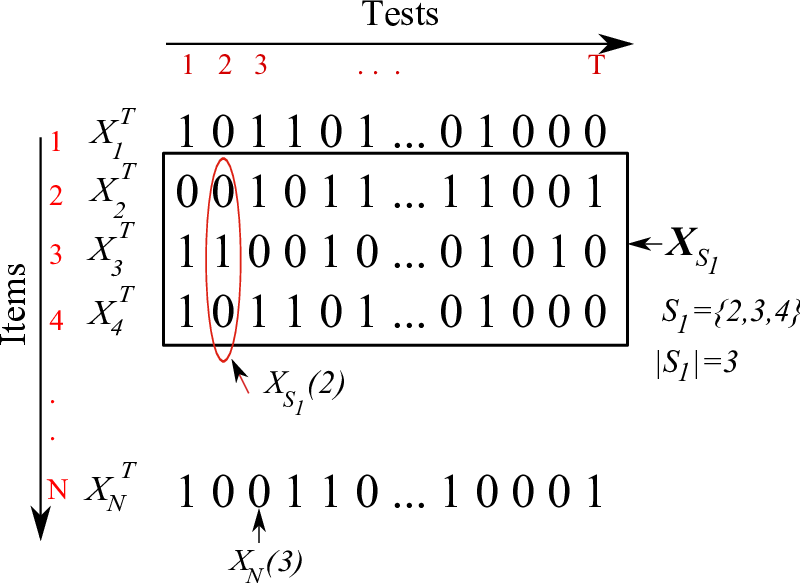
We use bold-face to denote matrices, while regular font is used to denote vectors, scalars and entries of matrices. For clarity, Fig. 2 illustrates our notation by means of a simple example.

  • •

    NN is the total number of items, KK is the known number of defectives (or positive items), pp denotes the probability that an item is part of a given test, and TT is the total number of tests.

  • •

    Codewords: For the jj-th item, XjTX_{j}^{T} is a binary row vector ∈{0,1}T\in\{0,1\}^{T}, with the tt-th entry Xj​(t)=1X_{j}(t)=1 if the jj-th item is pooled in test tt, and 00 otherwise. Following an information theoretic convention, we call it the jj-th codeword. The observation vector YTY^{T} is a binary vector of length TT, with entries equal to 11 for the tests with positive outcome. Similarly, Y⁡(t)Y(t) denotes the tt-th component of the vector YTY^{T}.

  • •

    𝑿X: The N×TN\times T measurement matrix, or the codebook, is a collection of NN codewords defining the pool design, i.e., the assignment of items to tests. Note that

    𝑿=[X1T;X2T;…;XNT]\text{\boldmath{$X$}}=[X_{1}^{T};X_{2}^{T};\ldots;X_{N}^{T}]

    where each entry represents a row of the matrix 𝑿X.

  • •

    Given a subset S⊂{1,2​…​N}S\subset\{1,2\ldots N\} with cardinality |S||S|, the matrix 𝑿S\text{\boldmath{$X$}}_{S} is an |S|×T|S|\times T matrix formed from the rows indexed by SS. In other words, 𝑿S\text{\boldmath{$X$}}_{S} denotes the collection of codewords (each of length TT) corresponding to the items in SS. Similarly, XSX_{S} denotes a vector, whose components are restricted to the set of components indexed by SS. Thus, XSX_{S} is a column of the matrix 𝑿S\text{\boldmath{$X$}}_{S}. When indexing by test is needed, XS​(t)X_{S}(t) is used to specifically denote the tt-th column of the matrix 𝑿S\text{\boldmath{$X$}}_{S}, and Xj​(t)X_{j}(t) is the tt-th component of the vector XjTX_{j}^{T}.

  • •

    Index the different sets of items of size KK as SωS_{\omega} with index ω\omega. Since there are NN items in total, there are (NK)\binom{N}{K} such sets, hence

    ω∈ℐ={1,2,…​(NK)}\omega\in{\cal I}=\left\{1,2,\ldots\binom{N}{K}\right\} (1)

    Note that SωS_{\omega} is a set of KK indices corresponding to the ω\omega-th set of items. The empty set is denoted ∅\emptyset and “⋁\bigvee” is used to denote the Boolean OR operation.

  • •

    Hence 𝑿Sω\text{\boldmath{$X$}}_{S_{\omega}} is the matrix of codewords corresponding to the items in the index set SωS_{\omega}.

Refer to caption
Fig. 2: The figure illustrates the notation through a simple example. Rows are codewords of length TT for corresponding items (denoted XjTX_{j}^{T}). A defective set S1={2,3,4}S_{1}=\{2,3,4\} consists of items 2,32,3 and 44. The corresponding matrix 𝑿S1\text{\boldmath{$X$}}_{S_{1}} is formed from rows indexed by S1S_{1}, i.e., consists of rows 2,3,42,3,4. The figure also illustrates the notation XS1​(2)X_{S_{1}}(2) which refers to the vector indexed by the set S1S_{1} for test t=2t=2. XN​(3)X_{N}(3) refers to the 33-rd test for item NN. Since the matrix is generated i.i.d., the vector XS1X_{S_{1}} (without a test index) refers to a vector whose components are restricted to the set of components indexed by S1S_{1}.

II-B Noise-free case

For the noise-free case, the outcome of the tests YTY^{T} is deterministic. It is the Boolean sum of the codewords corresponding to the defective set 𝒢\cal G. In other words

YT=⋁i∈𝒢XiT.Y^{T}=\bigvee_{i\in{\cal G}}X_{i}^{T}. (2)

Alternatively, if Ri∈{0,1}R_{i}\in\{0,1\} is an indicator function for the ii-th item determining whether it belongs to the defective set, i.e., Ri=1R_{i}=1 if i∈𝒢i\in{\cal G} and Ri=0R_{i}=0 otherwise, then the outcome Y⁡(t)Y(t) of the tt-th test in the noise-free case can be written as

Y⁡(t)=⋁i=1NXi​(t)​RiY(t)=\bigvee_{i=1}^{N}X_{i}(t)R_{i} (3)

where Xi​(t)X_{i}(t) is the tt-th entry of the vector XiTX_{i}^{T}, or equivalently, the binary entry at cell (i,t)(i,t) of the measurement matrix 𝑿X.

II-C Noisy cases

In this paper we also consider two noisy models, the additive model and the dilution model. However, we point out that our main achievability result is general and is not restricted to these specific noise models or to Boolean channels.

  • •

    Additive Model: In this model we account for false alarms in the outcome of pooling tests. The outcome of a test can still be 11 even if no positive items are pooled in that test. This effect is captured by adding independent Bernoulli(q)(q) random variables W⁡(t)W(t) to the outcome of the tt-th test of the noise-free model in Eq.(3), i.e.,

    Y⁡(t)=(⋁i=1NXi​(t)​Ri)∨W⁡(t)Y(t)=\left(\bigvee_{i=1}^{N}X_{i}(t)R_{i}\right)\vee W(t) (4)

    where W⁡(t)∼Bernoulli​(q),t=1​…​TW(t)\sim\mbox{Bernoulli}(q),t=1\ldots T.

  • •

    Dilution Model: The dilution model refers to the case when a defective item in a pool gets diluted. If all positive items in a given test appear as absent, that could potentially lead to erroneously zero outcomes. This model is motivated by blood dilution due to pooling with other negative tests or imperfectly diluted blood samples. This effect is captured by the Z-channel model of Fig.3. A Z-channel with crossover probability uu is a binary-input-binary-output channel that flips the input bit 11 with probability uu, but maps input bit 00 to 00 with probability 11 (for different Z-channel models the roles of 00 and 11 may be interchanged) [31]. In the dilution context, the input 11 corresponds to the inclusion of a positive item in a test while input 00 corresponds to the item being absent in that test. The asymmetric crossover captures the dilution effect, that is, in this model we might have misses but no false alarms. The outcome of the tt-th test can be written as:

    Y⁡(t)=⋁i=1N𝒵⁡(Xi​(t)​Ri)\displaystyle Y(t)=\bigvee_{i=1}^{N}{\cal Z}(X_{i}(t)R_{i}) (5)

where 𝒵\cal Z represents the Z-channel model of Fig. 3. Note that each term on the right hand side is crossed over independently according to this Z-channel model.

Refer to caption
Fig. 3: Dilution channel (Z-channel): positive items taking part in a given test might probabilistically behave as absent (diluted). In other words, even though a positive item is contained in a given pool, the test’s outcome could be negative if the item’s presence gets diluted for that specific test. For example, in blood testing the positive sample might get diluted in one or more tests leading to potential misses of infected blood samples.

Note that in the additive model, the outcome of testing a pool with no defective items might be erroneously positive, i.e., false positives would occur. On the other hand, the membership of a defective item in a given test might go unnoticed in the dilution model. If all defectives appearing in a given pool are diluted, a false negative occurs. The effect of dilution on the increase in number of tests is expected to be more severe than the effect of additive noise. This is explained by the fact that tests with negative outcomes are generally more informative; while a truly positive test merely indicates that at least one defective is present in the pool, a truly negative test exonerates all the members pooled in that test. With additive noise, a test with a negative outcome is never erroneous. In contrast, dilution diminishes our confidence in pools with negative outcomes, since a seemingly negative outcome would not necessarily mean all pooled members are perfect. Intuitively speaking, additive noise can be potentially mitigated by repetition of tests whereas the dilution effect is more intricate to resolve. This intuition is verified by the results we obtained through theoretical analysis as will be shown in the next sections.

II-D Performance criteria

The different sets of items of size KK are indexed SωS_{\omega}, where ω∈ℐ={1,2,…​(NK)}\omega\in{\cal I}=\{1,2,\ldots\binom{N}{K}\}. Define a decoding function g(.):𝒴T→ℐg(.):{\cal Y}^{T}\rightarrow{\cal I}. The function g(.)g(.) maps the outcome of the TT tests, YT∈𝒴TY^{T}\in{\cal Y}^{T}, to an index ω∈ℐ\omega\in{\cal I} corresponding to a specific set of defectives SωS_{\omega}. Now define the conditional error probability λω\lambda_{\omega} as

λω=Pr[g(YT)≠ω|𝒢=Sω,𝑿Sω]=∑YTpω(YT|𝑿Sω)1{g(YT)≠ω}\lambda_{\omega}=\Pr[g(Y^{T})\neq\omega|{\cal G}=S_{\omega},\text{\boldmath{$X$}}_{S_{\omega}}]=\sum_{Y^{T}}p_{\omega}(Y^{T}|\text{\boldmath{$X$}}_{S_{\omega}})\mbox{$1\!\!1$}{\{g(Y^{T})\neq\omega\}} (6)

where 1{.}\mbox{$1\!\!1$}{\{.\}} is an indicator function which takes the value 11 when its argument is realized and 00 otherwise, i.e., it takes the value 11 when the defective set is misclassified. The conditional probability pω​(YT|𝑿Sω)p_{\omega}(Y^{T}|\text{\boldmath{$X$}}_{S_{\omega}}) is the probability that YTY^{T} is the outcome of the TT tests given that SωS_{\omega} is the defective set with corresponding codewords matrix 𝑿Sω\text{\boldmath{$X$}}_{S_{\omega}}. The conditional probability defines a group testing channel which is analogous to a communication channel where the output sequence depends on the transmitted input sequence, the message being the defective set and the encoded sequence being the matrix of codewords corresponding to that set. The probability λω\lambda_{\omega} is the probability of error conditioned on a given defective set ω\omega and the codeword set, i.e., the probability that the decoded set is not the true defective set given that SωS_{\omega} is the true defective set with codeword set 𝑿Sω\text{\boldmath{$X$}}_{S_{\omega}}. Note that for the deterministic noise-free case this simplifies to λω=1{g(YT)≠ω}\lambda_{\omega}=\mbox{$1\!\!1$}{\{g(Y^{T})\neq\omega\}}. Averaging over all possible inputs ω\omega, we define the average error probability λ\lambda as:

λ=1(NK)​∑ωλω\lambda=\frac{1}{\binom{N}{K}}\sum_{\omega}\lambda_{\omega} (7)

For the aforementioned models (noiseless and noisy), we prove achievable and converse bounds on the total number of tests TT as N,K→∞N,K\rightarrow\infty. Namely, we consider the following criteria:

  • •

    Arbitrarily small average error probability33 3 We follow the standard reasoning approach in [23, 31] where we consider the error probability averaged all codebook realizations. An arbitrarily small average error probability in turn implies the existence of at least one good codebook.:

    λ=1(NK)​∑ωλω\lambda=\frac{1}{\binom{N}{K}}\sum_{\omega}\lambda_{\omega}
  • •

    Worst-case error probability:

    λmax=maxω⁡λω\lambda_{\max}=\max_{\omega}\lambda_{\omega}
  • •

    Partial reconstruction: In this case, we are satisfied with approximate reconstruction of the defective set. Let dd be a distance function between the decoded set g⁡(YT)g(Y^{T}) and the index ω\omega of the true defective set such that d⁡(g⁡(YT),ω)d(g(Y^{T}),\omega) is equal to the number of misses. Hence, if g⁡(YT)=ω^g(Y^{T})=\hat{\omega}, then

    d⁡(g⁡(YT),ω)=|Sω\Sω^|d(g(Y^{T}),\omega)=|S_{\omega}\backslash S_{\hat{\omega}}|

    is the cardinality of the set of missed items. Given KK declared candidates, an error occurs only if the number of missed items is greater than α​K\alpha K, i.e.,

    λω=∑YTpω(YT|𝑿Sω)1{d(g(YT),ω)>αK}\lambda_{\omega}=\sum_{Y^{T}}p_{\omega}(Y^{T}|\text{\boldmath{$X$}}_{S_{\omega}})\mbox{$1\!\!1$}{\{d(g(Y^{T}),\omega)>\alpha K\}}

In the following section we will derive our main result. We will prove a sufficient condition on the number of tests TT. The result is general as it applies to the noise-free and the noisy versions of the problem as we elaborate in the following sections.

III Main Result: Achievable bound

To derive an achievable bound on the number of tests TT, we show how the group testing problem can be mapped to an equivalent channel model. Using random coding and maximum likelihood decoding we upper bound the error probability, i.e., the probability of misclassifying the defective set.

III-A Random matrix generation and the encoding process

The binary measurement matrix is randomly generated. Associated with each item is a codeword that represents its assignment to tests. Assume that the codewords are generated randomly and independently according to some distribution qTq_{T}. The probability of a particular codebook 𝑿X assigning one codeword to each of the NN items, is Q⁡(𝑿)=∏j=1NqT​(XjT)Q(\text{\boldmath{$X$}})=\prod_{j=1}^{N}q_{T}(X_{j}^{T}), where qTq_{T} is a probability assignment on the set of input sequences of length TT. Since we will be assuming independence across tests and across items, to simplify notation we will use Q⁡(𝑭)Q(\text{\boldmath{$F$}}) to denote the distribution of a matrix 𝑭F of arbitrary size such that

Q⁡(𝑭)=∏i=1n1∏t=1n2q⁡(Fi​(t))Q(\text{\boldmath{$F$}})=\prod_{i=1}^{n_{1}}\prod_{t=1}^{n_{2}}q(F_{i}(t))

where FF is an n1×n2n_{1}\times n_{2} matrix with n1∈{1,…​N}n_{1}\in\{1,\ldots N\} and n2∈{1,…​T}n_{2}\in\{1,\ldots T\} and q​(Fi​(t))q(F_{i}(t)) denotes the distribution of the (i,t)(i,t)-th entry.

A defective set SωS_{\omega} corresponds to a collection of KK codewords, which is a K×TK\times T matrix 𝑿Sω\text{\boldmath{$X$}}_{S_{\omega}}, and can be thought of as an encoded message transmitted through the group testing channel. In other words, the encoder f:ℐ→{0,1}K×Tf:{\cal I}\rightarrow\{0,1\}^{K\times T}, maps an index ω∈ℐ\omega\in{\cal I} (defective set SωS_{\omega}) to a matrix of codewords 𝑿Sω∈{0,1}K×T\text{\boldmath{$X$}}_{S_{\omega}}\in\{0,1\}^{K\times T}, where {0,1}K×T\{0,1\}^{K\times T} is the space of binary K×TK\times T matrices. The encoded message f⁡(ω)=𝑿Sωf(\omega)=\text{\boldmath{$X$}}_{S_{\omega}} is then transmitted through a channel with transition probability pω​(YT|𝑿Sω)p_{\omega}(Y^{T}|\text{\boldmath{$X$}}_{S_{\omega}}) conditioned on the event 𝒢=Sω{\cal G}=S_{\omega}. The channel model is illustrated in Fig.4.

Refer to caption
Fig. 4: A set SS is the message that gets mapped to a code 𝑿S\text{\boldmath{$X$}}_{S}. The encoded message is transmitted through the group testing channel and produces the output YTY^{T}.

Since the channel is memoryless, i.e., each test outcome Y⁡(t)Y(t) depends only on the corresponding input XSω​(t)X_{S_{\omega}}(t), the probability of the output sequence YT=(Y⁡(1),Y⁡(2),…,Y⁡(T))Y^{T}=(Y(1),Y(2),\ldots,Y(T)) given the input 𝑿Sω=(XSω​(1),XSω​(2),…,XSω​(T))\text{\boldmath{$X$}}_{S_{\omega}}=(X_{S_{\omega}}(1),X_{S_{\omega}}(2),\ldots,X_{S_{\omega}}(T)) is given by

pω​(YT|𝑿Sω)=∏t=1Tpω​(Y⁡(t)|XSω​(t)).p_{\omega}(Y^{T}|\text{\boldmath{$X$}}_{S_{\omega}})=\prod_{t=1}^{T}p_{\omega}(Y(t)|X_{S_{\omega}}(t)).

Conditioned on the event 𝒢=Sω{\cal G}=S_{\omega} the KK codewords and the observed YTY^{T} have a joint distribution

pω​(𝑿Sω,YT)=∏t=1TQ⁡(XSω​(t))​pω​(Y⁡(t)|XSω​(t))p_{\omega}(\text{\boldmath{$X$}}_{S_{\omega}},Y^{T})=\prod_{t=1}^{T}Q(X_{S_{\omega}}(t))p_{\omega}(Y(t)|X_{S_{\omega}}(t))

Unless needed for clarity, we will often drop the suffix ω\omega in pω​(YT|𝑿Sω)p_{\omega}(Y^{T}|\text{\boldmath{$X$}}_{S_{\omega}}) to simplify notation since the conditioning index will be generally clear.

III-B Decoder

Decoding is achieved using ML decoding  [31]. The decoder goes through all (NK)\binom{N}{K} possible sets of size KK, where KK is the size of the defective set, and chooses the set that is most likely. The decoding rule is thus defined by: given the tests’outcomes YTY^{T}, choose ω∗\omega^{*} for which

p⁡(YT|𝑿Sω∗)>p⁡(YT|𝑿Sω);∀ω≠ω∗p(Y^{T}|\text{\boldmath{$X$}}_{S_{\omega^{*}}})>p(Y^{T}|\text{\boldmath{$X$}}_{S_{\omega}});~~~~\forall\omega\neq\omega^{*} (8)

i.e., choose the set for which the given YTY^{T} is most likely44 4 When two or more sets are in tie, the decoder can choose any of those sets. This is accounted for in the probability of error analysis. given ω\omega. An error occurs if any set other than the true defective set is more likely. This ML decoder minimizes the error probability assuming uniform prior on the input messages (defective sets). Next, we derive an upper bound on the average error probability of the ML decoder, where the average is taken over defective sets and ensembles of codewords.

III-C Probability of error analysis

Given the random codebook generation, let PeP_{e} denote the average probability of error, averaged over all codebooks 𝑿X, and over all sets of size KK, i.e.,

Pe\displaystyle P_{e} =\displaystyle= ∑𝑿Q⁡(𝑿)​λ​(𝑿)\displaystyle\sum_{\text{\boldmath{$X$}}}Q({\text{\boldmath{$X$}}})\lambda({\text{\boldmath{$X$}}}) (9)
=\displaystyle= ∑𝑿Q⁡(𝑿)​1(NK)​∑ωλω​(𝑿)\displaystyle\sum_{\text{\boldmath{$X$}}}Q({\text{\boldmath{$X$}}})\frac{1}{\binom{N}{K}}\sum_{\omega}\lambda_{\omega}({\text{\boldmath{$X$}}})
=\displaystyle= 1(NK)​∑ω∑𝑿Q⁡(𝑿)​λω​(𝑿)\displaystyle\frac{1}{\binom{N}{K}}\sum_{\omega}\sum_{\text{\boldmath{$X$}}}Q({\text{\boldmath{$X$}}})\lambda_{\omega}({\text{\boldmath{$X$}}})

By symmetry of the codebook construction, ∑𝑿Q⁡(𝑿)​λω​(𝑿)\sum_{\text{\boldmath{$X$}}}Q({\text{\boldmath{$X$}}})\lambda_{\omega}({\text{\boldmath{$X$}}}) does not depend on ω\omega (and consequently not on the set SωS_{\omega}). Thus,

Pe=∑𝑿Q⁡(𝑿)​λω​(𝑿)=Pe|ωP_{e}=\sum_{\text{\boldmath{$X$}}}Q({\text{\boldmath{$X$}}})\lambda_{\omega}({\text{\boldmath{$X$}}})=P_{e|\omega} (10)

where Pe|ωP_{e|\omega} is the error probability conditioned on ω\omega averaged over all codebooks. In other words, the average error probability does not depend on the input ω\omega due to averaging over randomly generated codebooks. Hence, if ω0\omega_{0} is the index of the true defective set we can assume without loss of generality that ω0=1\omega_{0}=1, i.e., S1S_{1} is the true defective set.

To simplify the exposition we introduce some further notation. As pointed out earlier, the matrix 𝑿S\text{\boldmath{$X$}}_{S} is formed from rows indexed by the set SS. For any 22 sets SiS_{i} and SjS_{j}, we define Si,jS_{i,j}, Sic,jS_{i^{c},j}, and Si,jcS_{i,j^{c}} as the overlap set, the set of indices in SjS_{j} but not in SiS_{i}, and the set of indices in SiS_{i} but not in SjS_{j}, respectively. Namely,

Si,j\displaystyle S_{i,j} =Si∩Sj​ overlap\displaystyle=S_{i}\cap S_{j}\mbox{~~~overlap}
Sic,j\displaystyle S_{i^{c},j} =Sic∩Sj​ in j but not in i\displaystyle=S_{i}^{c}\cap S_{j}\mbox{~~~in $j$ but not in $i$}
Si,jc\displaystyle S_{i,j^{c}} =Si∩Sjc​ in i but not in j\displaystyle=S_{i}\cap S_{j}^{c}\mbox{~~~in $i$ but not in $j$}

Now define the error event EiE_{i} as the event that a set which differs from the defective set S1S_{1} in exactly ii items is selected by the decoder. The probability of such an event is denoted P⁡(Ei)P(E_{i}). The event EiE_{i} implies that there exists some set which differs from the defective set in ii items and is more likely. Hence,

P(Ei)≤Pr[\displaystyle P(E_{i})\leq\Pr\Big[ ∃j≠1:pj​(YT|𝑿Sj)≥p1​(YT|𝑿S1)\displaystyle\exists j\neq 1:p_{j}(Y^{T}|\text{\boldmath{$X$}}_{S_{j}})\geq p_{1}(Y^{T}|\text{\boldmath{$X$}}_{S_{1}})
where|S1c,j|=|S1,jc|=i,and|S1|=|Sj|=K]\displaystyle\mbox{where}~~|S_{1^{c},j}|=|S_{1,j^{c}}|=i,~\mbox{and}~~|S_{1}|=|S_{j}|=K\Big] (11)

The probability P⁡(Ei)P(E_{i}) can be written as a summation over all inputs 𝑿S1\text{\boldmath{$X$}}_{S_{1}} and all test outcomes YTY^{T}

P(Ei)=∑𝑿S1∑YTQ(𝑿S1)p1(YT|𝑿S1)Pr[Ei|ω0=1,𝑿S1,YT]P(E_{i})=\sum_{\text{\boldmath{$X$}}_{S_{1}}}\sum_{Y^{T}}Q(\text{\boldmath{$X$}}_{S_{1}})p_{1}(Y^{T}|\text{\boldmath{$X$}}_{S_{1}})\Pr[E_{i}|\omega_{0}=1,\text{\boldmath{$X$}}_{S_{1}},Y^{T}] (12)

where Pr[Ei|ω0=1,𝑿S1,YT]\Pr[E_{i}|\omega_{0}=1,\text{\boldmath{$X$}}_{S_{1}},Y^{T}] is the probability of decoding error in exactly ii items, conditioned on message ω0=1\omega_{0}=1, the selection of a particular 𝑿S1\text{\boldmath{$X$}}_{S_{1}} as the codewords for the set S1S_{1}, and on the reception of a sequence YTY^{T}.

Using the union bound, the conditional error probability averaged over ensembles of codewords is upper bounded by,

Pe|1\displaystyle P_{e|1} ≤∑i=1KP⁡(Ei)\displaystyle\leq\sum_{i=1}^{K}P(E_{i})
=∑i=1K∑𝑿S1∑YTQ(𝑿S1)p(YT|𝑿S1)Pr[Ei|ω0=1,𝑿S1,YT]\displaystyle=\sum_{i=1}^{K}\sum_{\text{\boldmath{$X$}}_{S_{1}}}\sum_{Y^{T}}Q(\text{\boldmath{$X$}}_{S_{1}})p(Y^{T}|\text{\boldmath{$X$}}_{S_{1}})\Pr[E_{i}|\omega_{0}=1,\text{\boldmath{$X$}}_{S_{1}},Y^{T}] (13)

Next we state our main result. We need to introduce new notation to describe the result. Define ΞS{i}\Xi_{S}^{\{i\}} as the set of tuples (𝒮1,𝒮2)({\cal S}^{1},{\cal S}^{2}) partitioning the defective set SS into disjoint sets 𝒮1{\cal S}^{1} and 𝒮2{\cal S}^{2} with cardinalities ii and K−iK-i, respectively, i.e.,

ΞS{i}={(𝒮1,𝒮2):𝒮1⋂𝒮2=∅,𝒮1⋃𝒮2=S,|𝒮1|=i,|𝒮2|=K−i}\displaystyle\Xi_{S}^{\{i\}}=\left\{({\cal S}^{1},{\cal S}^{2}):{\cal S}^{1}\bigcap{\cal S}^{2}=\emptyset,{\cal S}^{1}\bigcup{\cal S}^{2}=S,|{\cal S}^{1}|=i,|{\cal S}^{2}|=K-i\right\} (14)

We let I⁡(X𝒮1,X𝒮2,Y)I(X_{{\cal S}^{1}};X_{{\cal S}^{2}},Y) denote the mutual information [23] between X𝒮1X_{{\cal S}^{1}} and (X𝒮2,Y)(X_{{\cal S}^{2}},Y) defined as,

I⁡(X𝒮1,X𝒮2,Y)=∑Y∑X𝒮2∑X𝒮1Q⁡(X𝒮1)​p​(Y,X𝒮2|X𝒮1)​log⁡p⁡(Y,X𝒮2|X𝒮1)∑X𝒮1Q⁡(X𝒮1)​p​(Y,X𝒮2|X𝒮1).\displaystyle I(X_{{\cal S}^{1}};X_{{\cal S}^{2}},Y)=\sum_{Y}\sum_{X_{{\cal S}^{2}}}\sum_{X_{{\cal S}^{1}}}Q(X_{{\cal S}^{1}})p(Y,X_{{\cal S}^{2}}|X_{{\cal S}^{1}})\log\frac{p(Y,X_{{\cal S}^{2}}|X_{{\cal S}^{1}})}{\sum_{X_{{\cal S}^{1}}}Q(X_{{\cal S}^{1}})p(Y,X_{{\cal S}^{2}}|X_{{\cal S}^{1}})}\,\,.

The following theorem provides a sufficient condition on the number of tests TT for an arbitrarily small average error probability.

Theorem III.1

(Sufficiency). Let NN be the size of a population of items with the defective set SS of cardinality KK. If the number tests TT is such that

T>(1+ϵ)⋅maxi:(𝒮1,𝒮2)∈ΞS{i}log⁡(N−Ki)​(Ki)I⁡(X𝒮1,X𝒮2,Y),i=1,2,…K\displaystyle T>(1+\epsilon)\cdot\max_{i:({\cal S}^{1},{\cal S}^{2})\in\Xi_{S}^{\{i\}}}\frac{\log\binom{N-K}{i}\binom{K}{i}}{I(X_{{\cal S}^{1}};X_{{\cal S}^{2}},Y)},~~i=1,2,\ldots K (15)

then asymptotically the average error probability approaches zero, namely,

limK→∞limN→∞Pe→0\displaystyle\lim_{K\rightarrow\infty}\lim_{N\rightarrow\infty}P_{e}\rightarrow 0 (16)

where ϵ>0\epsilon>0 is a constant independent of NN and KK.

Remark III.1

Theorem III.1 provides a sufficient condition for the case where NN scales to infinity for every fixed K. The question arises as to what happens when both NN and KK scale at the same rate. We will describe this case in Section III-F.

Theorem III.1 follows from a tight bound—based on characterization of error exponents as in [31]—on the error probability P⁡(Ei)P(E_{i}). We will show that the error exponent, Eo​(ρ)E_{o}(\rho), is described by:

Eo(ρ)=−log∑Y∈{0,1}∑X𝒮2[∑X𝒮1Q(X𝒮1)p(Y,X𝒮2|X𝒮1)11+ρ]1+ρ0≤ρ≤1\displaystyle E_{o}(\rho)=-\log\sum_{Y\in\{0,1\}}\sum_{X_{{\cal S}^{2}}}\left[\sum_{X_{{\cal S}^{1}}}Q(X_{{\cal S}^{1}})p(Y,X_{{\cal S}^{2}}|X_{{\cal S}^{1}})^{\frac{1}{1+\rho}}\right]^{1+\rho}~~~0\leq\rho\leq 1 (17)

where, (𝒮1,𝒮2)∈ΞS{i}({\cal S}^{1},{\cal S}^{2})\in\Xi_{S}^{\{i\}}, defined in (14), denote any disjoint partitions of the defective set S1S_{1} with cardinalities ii and K−iK-i, respectively. X𝒮1X_{{\cal S}^{1}} and X𝒮2X_{{\cal S}^{2}} are the corresponding disjoint partitions of the K×1K\times 1 input XS1X_{S_{1}} of lengths i×1i\times 1 and (K−i)×1(K-i)\times 1, respectively. We then have the following result:

Lemma III.1

The probability of the error event EiE_{i} defined in Eq. 12 that a set which differs from the defective set S1S_{1} in exactly ii items is selected by the ML decoder (averaged over all codebooks and test outcomes) is bounded from above by

P⁡(Ei)≤2−T⁡(Eo​(ρ)−ρ​log⁡(N−Ki)​(Ki)T)\displaystyle P(E_{i})\leq 2^{-T\left(E_{o}(\rho)-\rho\frac{\log\binom{N-K}{i}\binom{K}{i}}{T}\right)} (18)

We are now ready to prove Theorem III.1.

III-D Proof of Theorem III.1

Now we can readily prove our main result. First, we need to derive a sufficient condition for the error exponent of the error probability P⁡(Ei)P(E_{i}) in (18) to be positive and to drive the error probability to zero as N→∞N\rightarrow\infty. Specifically,

T​f​(ρ)=T​Eo​(ρ)−ρ​log⁡(N−Ki)​(Ki)→∞\displaystyle Tf(\rho)=TE_{o}(\rho)-\rho\log\binom{N-K}{i}\binom{K}{i}\rightarrow\infty (19)

where

f⁡(ρ)=Eo​(ρ)−ρ​log⁡(N−Ki)​(Ki)Tf(\rho)=E_{o}(\rho)-\rho\frac{\log\binom{N-K}{i}\binom{K}{i}}{T}

and where Eo​(ρ)E_{o}(\rho) is defined in (17).

To establish Eq. 15 we follow the argument in [31]. Note that f⁡(0)=0f(0)=0. Since the function f⁡(ρ)f(\rho) is differentiable and has a power series expansion, for a sufficiently small δ\delta, we get by Taylor series expansion in the neighborhood of ρ∈[0,δ]\rho\in[0,\delta] that,

f⁡(ρ)=f⁡(0)+ρ​d​fd​ρ|ρ=0+O⁡(ρ2)f(\rho)=f(0)+\rho\frac{df}{d\rho}\Big|_{\rho=0}+O(\rho^{2})

But we can show that

∂Eo∂ρ|ρ=0=∑Y∑X𝒮2[\displaystyle\frac{\partial E_{o}}{\partial\rho}\Big|_{\rho=0}=\sum_{Y}\sum_{X_{{\cal S}^{2}}}\Bigg[ ∑X𝒮1Q⁡(X𝒮1)​p​(Y,X𝒮2|X𝒮1)​log⁡p⁡(Y,X𝒮2|X𝒮1)\displaystyle\sum_{X_{{\cal S}^{1}}}Q(X_{{\cal S}^{1}})p(Y,X_{{\cal S}^{2}}|X_{{\cal S}^{1}})\log p(Y,X_{{\cal S}^{2}}|X_{{\cal S}^{1}})
−\displaystyle- ∑X𝒮1Q(X𝒮1)p(Y,X𝒮2|X𝒮1)log∑X𝒮1Q(X𝒮1)p(Y,X𝒮2|X𝒮1)]\displaystyle\sum_{X_{{\cal S}^{1}}}Q(X_{{\cal S}^{1}})p(Y,X_{{\cal S}^{2}}|X_{{\cal S}^{1}})\log\sum_{X_{{\cal S}^{1}}}Q(X_{{\cal S}^{1}})p(Y,X_{{\cal S}^{2}}|X_{{\cal S}^{1}})\Bigg] (20)

which simplifies to

∂Eo∂ρ|ρ=0\displaystyle\frac{\partial E_{o}}{\partial\rho}\Big|_{\rho=0} =∑Y∑X𝒮2∑X𝒮1Q⁡(X𝒮1)​p​(Y,X𝒮2|X𝒮1)​log⁡p⁡(Y,X𝒮2|X𝒮1)∑X𝒮1Q⁡(X𝒮1)​p​(Y,X𝒮2|X𝒮1)\displaystyle=\sum_{Y}\sum_{X_{{\cal S}^{2}}}\sum_{X_{{\cal S}^{1}}}Q(X_{{\cal S}^{1}})p(Y,X_{{\cal S}^{2}}|X_{{\cal S}^{1}})\log\frac{p(Y,X_{{\cal S}^{2}}|X_{{\cal S}^{1}})}{\sum_{X_{{\cal S}^{1}}}Q(X_{{\cal S}^{1}})p(Y,X_{{\cal S}^{2}}|X_{{\cal S}^{1}})}
=I⁡(X𝒮1,X𝒮2,Y)\displaystyle=I(X_{{\cal S}^{1}};X_{{\cal S}^{2}},Y) (21)

Now it is easy to see that with (1+ϵ)​log⁡(N−Ki)​(Ki)T<I⁡(X𝒮1,X𝒮2,Y)(1+\epsilon)\frac{\log\binom{N-K}{i}\binom{K}{i}}{T}<I(X_{{\cal S}^{1}};X_{{\cal S}^{2}},Y) for some constant ϵ>0\epsilon>0, the condition in (19) is satisfied, i.e., T​f​(ρ)→∞Tf(\rho)\rightarrow\infty as N→∞N\rightarrow\infty. To argue this we first note that from the Lagrange form of the Taylor Series expansion (an application of the mean value theorem) we can write Eo​(ρ)E_{o}(\rho) in terms of its first derivative evaluated at zero and a remainder term, i.e.,

Eo​(ρ)=Eo​(0)+ρ​Eo′​(0)+ρ22​Eo′′​(ψ)\displaystyle E_{o}(\rho)=E_{o}(0)+\rho E_{o}^{\prime}(0)+{\rho^{2}\over 2}E_{o}^{\prime\prime}(\psi) (22)

for some ψ∈[0,ρ]\psi\in[0,\rho]. Hence, for the choice of TT in (15) we have

T​f​(ρ)≥T⁡(ρ​ϵ1+ϵ​I​(X𝒮1,X𝒮2,Y)−ρ2​C​I​(X𝒮1,X𝒮2,Y))\displaystyle Tf(\rho)\geq T\left(\rho\frac{\epsilon}{1+\epsilon}I(X_{{\cal S}^{1}};X_{{\cal S}^{2}},Y)-\rho^{2}CI(X_{{\cal S}^{1}};X_{{\cal S}^{2}},Y)\right)

where C=−|Eo′′​(ψ)|I⁡(X𝒮1,X𝒮2,Y)C=-\frac{|E_{o}^{\prime\prime}(\psi)|}{I(X_{{\cal S}^{1}};X_{{\cal S}^{2}},Y)} which might depend on KK. Note that, CC being a continuous function is bounded on the closed unit interval. Now if we choose ρ≤ϵ′C\rho\leq\frac{\epsilon^{\prime}}{C}, where ϵ′=ϵ1+ϵ\epsilon^{\prime}=\frac{\epsilon}{1+\epsilon}, then f⁡(ρ)=δf(\rho)=\delta for some δ>0\delta>0 which does not depend on NN or TT. It follows that T​f​(ρ)→∞Tf(\rho)\rightarrow\infty as N→∞N\rightarrow\infty.

We have just shown that for fixed KK, T>(1+ϵ)⋅log⁡(N−Ki)​(Ki)I⁡(X𝒮1,X𝒮2,Y)T>(1+\epsilon)\cdot\frac{\log\binom{N-K}{i}\binom{K}{i}}{I(X_{{\cal S}^{1}};X_{{\cal S}^{2}},Y)} is sufficient to ensure an arbitrarily small P⁡(Ei)P(E_{i}). Since the average error probability Pe≤∑i=1KP⁡(Ei)P_{e}\leq\sum_{i=1}^{K}P(E_{i}), it follows that for any fixed KK, limN→∞∑i=1KP⁡(Ei)=0\lim_{N\rightarrow\infty}\sum_{i=1}^{K}P(E_{i})=0. Consequently, since this is true for any KK, limK→∞limN→∞∑i=1KP⁡(Ei)=0\lim_{K\rightarrow\infty}\lim_{N\rightarrow\infty}\sum_{i=1}^{K}P(E_{i})=0. Theorem III.1 now follows.

III-E Proof of Lemma III.1

To build intuition we will first show the following weaker bound:

P⁡(Ei)≤2−T⁡(Eo​(ρ)−log⁡(N−Ki)​(Ki)T)\displaystyle P(E_{i})\leq 2^{-T\left(E_{o}(\rho)-\frac{\log\binom{N-K}{i}\binom{K}{i}}{T}\right)} (23)

Note that the main difference between the above equation and Lemma III.1 is the missing ρ\rho term multiplying the binomial expression. The main result follows along the same lines and is described in detail in the appendix. It is based on exploiting two types of symmetry: the symmetry of codebook construction; and the symmetry of the channel output to permutations of the rows of matrix 𝑿X. Note that it is possible to obtain qualitatively similar results as in Table I using this weaker bound. However, the expression in Theorem III.1 does not turn out to be as explicit with this bound.

To prove this weaker result we denote by 𝒜{\cal A}

𝒜={ω∈ℐ:|S1c,ω|=i,|Sω|=K}\displaystyle{\cal A}=\{\omega\in{\cal I}:|S_{1^{c},\omega}|=i,|S_{\omega}|=K\} (24)

the set of indices corresponding to sets of KK items that differ from the true defective set S1S_{1} in exactly ii items. We can establish that,

Pr[Ei|ω0=1,𝑿S1,YT]\displaystyle\Pr[E_{i}|\omega_{0}=1,\text{\boldmath{$X$}}_{S_{1}},Y^{T}] ≤∑ω∈𝒜∑𝑿S1c,ωQ⁡(𝑿S1c,ω)​pω​(YT,𝑿S1,ω|𝑿S1c,ω)sp1​(YT,𝑿S1,ω|𝑿S1,ωc)s\displaystyle\leq\sum_{\omega\in{\cal A}}\sum_{\begin{subarray}{c}\text{\boldmath{$X$}}_{S_{1^{c},\omega}}\end{subarray}}Q(\text{\boldmath{$X$}}_{S_{1^{c},\omega}})\frac{p_{\omega}(Y^{T},\text{\boldmath{$X$}}_{S_{1,\omega}}|\text{\boldmath{$X$}}_{S_{1^{c},\omega}})^{s}}{p_{1}(Y^{T},\text{\boldmath{$X$}}_{S_{1,\omega}}|\text{\boldmath{$X$}}_{S_{1,\omega^{c}}})^{s}} (25)
=∑S1,ω∑S1c,ω∑𝑿S1c,ωQ⁡(𝑿S1c,ω)​pω​(YT,𝑿S1,ω|𝑿S1c,ω)sp1​(YT,𝑿S1,ω|𝑿S1,ωc)s\displaystyle=\sum_{S_{1,\omega}}\sum_{S_{1^{c},\omega}}\sum_{\begin{subarray}{c}\text{\boldmath{$X$}}_{S_{1^{c},\omega}}\end{subarray}}Q(\text{\boldmath{$X$}}_{S_{1^{c},\omega}})\frac{p_{\omega}(Y^{T},\text{\boldmath{$X$}}_{S_{1,\omega}}|\text{\boldmath{$X$}}_{S_{1^{c},\omega}})^{s}}{p_{1}(Y^{T},\text{\boldmath{$X$}}_{S_{1,\omega}}|\text{\boldmath{$X$}}_{S_{1,\omega^{c}}})^{s}}

Inequality (25) is established in the Appendix. It follows that,

Pr[Ei|ω0=1,𝑿S1,YT]\displaystyle\Pr[E_{i}|\omega_{0}=1,\text{\boldmath{$X$}}_{S_{1}},Y^{T}] ≤(a)(∑S1,ω∑S1c,ω∑𝑿S1c,ωQ⁡(𝑿S1c,ω)​pω​(YT,𝑿S1,ω|𝑿S1c,ω)sp1​(YT,𝑿S1,ω|𝑿S1,ωc)s)ρ\displaystyle\stackrel{{\scriptstyle(a)}}{{\leq}}\left(\sum_{S_{1,\omega}}\sum_{S_{1^{c},\omega}}\sum_{\begin{subarray}{c}\text{\boldmath{$X$}}_{S_{1^{c},\omega}}\end{subarray}}Q(\text{\boldmath{$X$}}_{S_{1^{c},\omega}})\frac{p_{\omega}(Y^{T},\text{\boldmath{$X$}}_{S_{1,\omega}}|\text{\boldmath{$X$}}_{S_{1^{c},\omega}})^{s}}{p_{1}(Y^{T},\text{\boldmath{$X$}}_{S_{1,\omega}}|\text{\boldmath{$X$}}_{S_{1,\omega^{c}}})^{s}}\right)^{\rho}
≤(b)(∑S1,ω(N−Ki)​∑𝑿S1c,ωQ⁡(𝑿S1c,ω)​pω​(YT,𝑿S1,ω|𝑿S1c,ω)sp1​(YT,𝑿S1,ω|𝑿S1,ωc)s)ρ\displaystyle\stackrel{{\scriptstyle(b)}}{{\leq}}\left(\sum_{S_{1,\omega}}\binom{N-K}{i}\sum_{\begin{subarray}{c}\text{\boldmath{$X$}}_{S_{1^{c},\omega}}\end{subarray}}Q(\text{\boldmath{$X$}}_{S_{1^{c},\omega}})\frac{p_{\omega}(Y^{T},\text{\boldmath{$X$}}_{S_{1,\omega}}|\text{\boldmath{$X$}}_{S_{1^{c},\omega}})^{s}}{p_{1}(Y^{T},\text{\boldmath{$X$}}_{S_{1,\omega}}|\text{\boldmath{$X$}}_{S_{1,\omega^{c}}})^{s}}\right)^{\rho}
≤(c)(N−Ki)​∑S1,ω(∑𝑿S1c,ωQ⁡(𝑿S1c,ω)​pω​(YT,𝑿S1,ω|𝑿S1c,ω)sp1​(YT,𝑿S1,ω|𝑿S1,ωc)s)ρ​∀s>0,  0≤ρ≤1\displaystyle\stackrel{{\scriptstyle(c)}}{{\leq}}\binom{N-K}{i}\sum_{S_{1,\omega}}\left(\sum_{\begin{subarray}{c}\text{\boldmath{$X$}}_{S_{1^{c},\omega}}\end{subarray}}Q(\text{\boldmath{$X$}}_{S_{1^{c},\omega}})\frac{p_{\omega}(Y^{T},\text{\boldmath{$X$}}_{S_{1,\omega}}|\text{\boldmath{$X$}}_{S_{1^{c},\omega}})^{s}}{p_{1}(Y^{T},\text{\boldmath{$X$}}_{S_{1,\omega}}|\text{\boldmath{$X$}}_{S_{1,\omega^{c}}})^{s}}\right)^{\rho}~~\forall s>0,\,\,0\leq\rho\leq 1

Inequality (a) follows from the fact that Pr[Ei|ω0=1,𝑿S1,YT]≤1\Pr[E_{i}|\omega_{0}=1,\text{\boldmath{$X$}}_{S_{1}},Y^{T}]\leq 1. Consequently, if UU is an upperbound of this probability then it follows that, Pr[Ei|ω0=1,𝑿S1,YT]≤Uρ\Pr[E_{i}|\omega_{0}=1,\text{\boldmath{$X$}}_{S_{1}},Y^{T}]\leq U^{\rho} for ρ∈[0,1]\rho\in[0,1]. Inequality (b) follows from symmetry of codebook construction, namely, the inner summation is only dependent on the values of 𝑿S1c,ω\text{\boldmath{$X$}}_{S_{1^{c},\omega}} and not on the items in the set S1c,ωS_{1^{c},\omega}. There are exactly (N−Ki)\binom{N-K}{i} possible sets S1c,ωS_{1^{c},\omega} hence the binomial expression. Note that the sum over S1,ωS_{1,\omega} cannot be further simplified. This is due to the fact that 𝑿S1,ω\text{\boldmath{$X$}}_{S_{1,\omega}} is already specified since we have conditioned on 𝑿S1\text{\boldmath{$X$}}_{S_{1}}. Since 𝑿S1\text{\boldmath{$X$}}_{S_{1}} is fixed, the inner sum need not be equal for all sets S1,ω,ω∈𝒜S_{1,\omega},\omega\in{\cal A}. Indeed, the main difference between the weaker and stronger bound is this issue. In the stronger bound we incorporate the symmetry both in the missed as well as common components. Finally, (c) follows from standard observation that sum of positive numbers raised to ρ\rho-th power for ρ<1\rho<1 is smaller than the sum of the ρ\rho-th power of each number.

We now substitute for the conditional error probability derived above and follow the steps below:

P⁡(Ei)\displaystyle P(E_{i}) =∑𝑿S1∑YTp1(𝑿S1,YT)Pr[Ei|ω0=1,𝑿S1,YT]\displaystyle=\sum_{\text{\boldmath{$X$}}_{S_{1}}}\sum_{Y^{T}}p_{1}(\text{\boldmath{$X$}}_{S_{1}},Y^{T})\Pr[E_{i}|\omega_{0}=1,\text{\boldmath{$X$}}_{S_{1}},Y^{T}]
≤(N−Ki)​∑S1,ω∑YT∑𝑿S1p1​(𝑿S1,YT)​(∑𝑿S1c,ωQ⁡(𝑿S1c,ω)​pω​(YT,𝑿S1,ω|𝑿S1c,ω)sp1​(YT,𝑿S1,ω|𝑿S1,ωc)s)ρ\displaystyle\leq\binom{N-K}{i}\sum_{S_{1,\omega}}\sum_{Y^{T}}\sum_{\text{\boldmath{$X$}}_{S_{1}}}p_{1}(\text{\boldmath{$X$}}_{S_{1}},Y^{T})\left(\sum_{\begin{subarray}{c}\text{\boldmath{$X$}}_{S_{1^{c},\omega}}\end{subarray}}Q(\text{\boldmath{$X$}}_{S_{1^{c},\omega}})\frac{p_{\omega}(Y^{T},\text{\boldmath{$X$}}_{S_{1,\omega}}|\text{\boldmath{$X$}}_{S_{1^{c},\omega}})^{s}}{p_{1}(Y^{T},\text{\boldmath{$X$}}_{S_{1,\omega}}|\text{\boldmath{$X$}}_{S_{1,\omega^{c}}})^{s}}\right)^{\rho}

Due to symmetry the summation over sets S1,ωS_{1,\omega} does not depend on ω\omega. Since there are (KK−i)\binom{K}{K-i} sets S1,ωS_{1,\omega} we get,

P⁡(Ei)\displaystyle P(E_{i}) ≤(N−Ki)​(Ki)​∑YT∑𝑿S1p1​(𝑿S1,YT)​(∑𝑿S1c,ωQ⁡(𝑿S1c,ω)​pω​(YT,𝑿S1,ω|𝑿S1c,ω)sp1​(YT,𝑿S1,ω|𝑿S1,ωc)s)ρ\displaystyle\leq\binom{N-K}{i}\binom{K}{i}\sum_{Y^{T}}\sum_{\text{\boldmath{$X$}}_{S_{1}}}p_{1}(\text{\boldmath{$X$}}_{S_{1}},Y^{T})\left(\sum_{\begin{subarray}{c}\text{\boldmath{$X$}}_{S_{1^{c},\omega}}\end{subarray}}Q(\text{\boldmath{$X$}}_{S_{1^{c},\omega}})\frac{p_{\omega}(Y^{T},\text{\boldmath{$X$}}_{S_{1,\omega}}|\text{\boldmath{$X$}}_{S_{1^{c},\omega}})^{s}}{p_{1}(Y^{T},\text{\boldmath{$X$}}_{S_{1,\omega}}|\text{\boldmath{$X$}}_{S_{1,\omega^{c}}})^{s}}\right)^{\rho}
≤(N−Ki)​(Ki)​∑YT∑𝑿S1,ωc∑𝑿S1,ωQ⁡(𝑿S1,ωc)​p1​(𝑿S1,ω,YT∣𝑿S1,ωc)\displaystyle\leq\binom{N-K}{i}\binom{K}{i}\sum_{Y^{T}}\sum_{\text{\boldmath{$X$}}_{S_{1,\omega^{c}}}}\sum_{\text{\boldmath{$X$}}_{S_{1,\omega}}}Q(\text{\boldmath{$X$}}_{S_{1,\omega^{c}}})p_{1}(\text{\boldmath{$X$}}_{S_{1,\omega}},Y^{T}\mid\text{\boldmath{$X$}}_{S_{1,\omega^{c}}})
(∑𝑿S1c,ωQ⁡(𝑿S1c,ω)​pω​(YT,𝑿S1,ω|𝑿S1c,ω)sp1​(YT,𝑿S1,ω|𝑿S1,ωc)s)ρ\displaystyle~~~~~~~~~~~~~~~~~~~~~~~~~~~~~~~~~~~~~~~~~~~~~~~~~~~~~~~~~~~\left(\sum_{\begin{subarray}{c}\text{\boldmath{$X$}}_{S_{1^{c},\omega}}\end{subarray}}Q(\text{\boldmath{$X$}}_{S_{1^{c},\omega}})\frac{p_{\omega}(Y^{T},\text{\boldmath{$X$}}_{S_{1,\omega}}|\text{\boldmath{$X$}}_{S_{1^{c},\omega}})^{s}}{p_{1}(Y^{T},\text{\boldmath{$X$}}_{S_{1,\omega}}|\text{\boldmath{$X$}}_{S_{1,\omega^{c}}})^{s}}\right)^{\rho}
=(N−Ki)​(Ki)​∑YT∑𝑿S1,ωc∑𝑿S1,ωQ⁡(𝑿S1,ωc)​p11−s​ρ​(𝑿S1,ω,YT∣𝑿S1,ωc)\displaystyle=\binom{N-K}{i}\binom{K}{i}\sum_{Y^{T}}\sum_{\text{\boldmath{$X$}}_{S_{1,\omega^{c}}}}\sum_{\text{\boldmath{$X$}}_{S_{1,\omega}}}Q(\text{\boldmath{$X$}}_{S_{1,\omega^{c}}})p_{1}^{1-s\rho}(\text{\boldmath{$X$}}_{S_{1,\omega}},Y^{T}\mid\text{\boldmath{$X$}}_{S_{1,\omega^{c}}})
(∑𝑿S1c,ωQ⁡(𝑿S1c,ω)​pω​(YT,𝑿S1,ω|𝑿S1c,ω)s)ρ\displaystyle~~~~~~~~~~~~~~~~~~~~~~~~~~~~~~~~~~~~~~~~~~~~~~~~~~~~~~~~~~~\left(\sum_{\begin{subarray}{c}\text{\boldmath{$X$}}_{S_{1^{c},\omega}}\end{subarray}}Q(\text{\boldmath{$X$}}_{S_{1^{c},\omega}})p_{\omega}(Y^{T},\text{\boldmath{$X$}}_{S_{1,\omega}}|\text{\boldmath{$X$}}_{S_{1^{c},\omega}})^{s}\right)^{\rho}
=(N−Ki)​(Ki)​∑YT∑𝑿S1,ω(∑𝑿S1,ωcQ⁡(𝑿S1,ωc)​p11/(1+ρ)​(𝑿S1,ω,YT∣𝑿S1,ωc))1+ρ\displaystyle=\binom{N-K}{i}\binom{K}{i}\sum_{Y^{T}}\sum_{\text{\boldmath{$X$}}_{S_{1,\omega}}}\left(\sum_{\text{\boldmath{$X$}}_{S_{1,\omega^{c}}}}Q(\text{\boldmath{$X$}}_{S_{1,\omega^{c}}})p_{1}^{1/(1+\rho)}(\text{\boldmath{$X$}}_{S_{1,\omega}},Y^{T}\mid\text{\boldmath{$X$}}_{S_{1,\omega^{c}}})\right)^{1+\rho}
=(N−Ki)​(Ki)​∑Y∑XS1,ω(∑XS1,ωcQ⁡(XS1,ωc)​p11/(1+ρ)​(XS1,ω,YT∣XS1,ωc))T⁡(1+ρ)\displaystyle=\binom{N-K}{i}\binom{K}{i}\sum_{Y}\sum_{X_{S_{1,\omega}}}\left(\sum_{X_{S_{1,\omega^{c}}}}Q(X_{S_{1,\omega^{c}}})p_{1}^{1/(1+\rho)}(X_{S_{1,\omega}},Y^{T}\mid X_{S_{1,\omega^{c}}})\right)^{T(1+\rho)}

where the last step follows due to independence of the tests. The step before the last follows by noting that from symmetry 𝑿S1c,ω\text{\boldmath{$X$}}_{S_{1^{c},\omega}} is just a dummy variable and can be replaced by 𝑿S1,ωc\text{\boldmath{$X$}}_{S_{1,\omega^{c}}}. This establishes the weaker bound in (23). Further details about the proof of Lemma III.1 are described in Appendix A.

III-F General case where K=o⁡(N)K=o(N)

We explicitly differentiate between two different scaling regimes considered in the paper. The result of Theorem III.1 we just presented provides a sufficient condition for the case where NN scales to infinity for every fixed K ensuring that

limK→∞limN→∞Pe→0.\lim_{K\rightarrow\infty}\lim_{N\rightarrow\infty}P_{e}\rightarrow 0.

As we mentioned earlier, since the error probability averaged over all codebooks is arbitrarily small, this in turn implies the existence of at least one good codebook and hence λ→0\lambda\rightarrow 0. However, we point out that the result in Theorem III.1 can be extended to the more general case where both NN and KK are allowed to scale simultaneously such that K=o⁡(N)K=o(N). From the Lagrange form of the Taylor Series expansion we can write Eo​(ρ)E_{o}(\rho) in terms of its first derivative evaluated at zero and a remainder term which depends on the second derivative (22). We have already shown that Eo​(0)=0E_{o}(0)=0 and Eo′​(0)=I⁡(X𝒮1;Y∣X𝒮2)>0E_{o}^{\prime}(0)=I(X_{{\cal S}^{1}};Y\mid X_{{\cal S}^{2}})>0. Consequently, we need to lower bound Eo​(ρ)E_{o}(\rho) by taking the worst-case second derivative. Establishing this result requires a more careful analysis and hence we present it in Appendix C. It is shown that the same sufficient condition on the number of tests TT in Theorem III.1 holds up to an extra polylog(KK) factor for an arbitrarily small average error probability, namely,

limN→∞K=o⁡(N)Pe→0\lim_{\begin{subarray}{c}N\rightarrow\infty\\ K=o(N)\end{subarray}}P_{e}\rightarrow 0

Relation to channel coding:
The mutual information I⁡(X𝒮1,X𝒮2,Y)I(X_{{\cal S}^{1}};X_{{\cal S}^{2}},Y) between X𝒮1X_{{\cal S}^{1}} and (X𝒮2,Y)(X_{{\cal S}^{2}},Y) is the relative entropy between the joint distribution p⁡(X𝒮1,X𝒮2,Y)p(X_{{\cal S}^{1}},X_{{\cal S}^{2}},Y) and the product distribution p⁡(X𝒮1)​p​(X𝒮2,Y)p(X_{{\cal S}^{1}})p(X_{{\cal S}^{2}},Y). It is a measure of the amount of information that the variables X𝒮2X_{{\cal S}^{2}} and YY contain about X𝒮1X_{{\cal S}^{1}}  [23]. Intuitively this means that the upper bound on the error probability P⁡(Ei)P(E_{i}), where the event EiE_{i} represents the event that the decoded set is misclassified in exactly ii items (replacing ii codewords of the true set with ii independent codewords), scales exponentially with the negative of the per-test mutual information between ii codewords of the set, and the remaining K−iK-i codewords and the output.

It is worthwhile mentioning that in the classical channel coding problem [31, 23], the error probability analysis for Maximum Likelihood or Typical Set Decoding separates well due to the independence of the channel output and every codeword other than the truly transmitted one. However, in the group testing problem, a main difficulty arises from the fact that an arbitrary set of KK items and the true defective set could be overlapping. Hence, independence of the output and the collection of codewords indexed by that set does not hold anymore. That required introducing the previous machinery to analyze the error probability. Two ingredients that were key to our analysis are

  1. 1.

    Separating the error events EiE_{i} of misclassifying the defective set in ii items

  2. 2.

    For every ii, we averaged over realizations of ensemble of codewords of every candidate set while holding fixed the partition common to these sets and the true set of defectives.

Further Intuition: Intuitively, the numerator in Theorem III.1 represents the number of bits required to enumerate all possible sets with ii misclassified items (ii out of KK), and the denominator represents the amount of information per test if K−iK-i of the defective items are known. One key idea behind the described approach is illustrated in Fig. 5. The group testing problem has been mapped to an equivalent multiple channel model. Each channel accounts for the case where K−iK-i of the defective items are recovered and ii items are still to be recognized, where K−iK-i represents the overlap between the true defective set and a false candidate set. The total error probability in decoding the true defective set depends on the decoding error probability for each channel. By studying each error channel separately, we upper bound the overall error probability.

Refer to caption
Fig. 5: Equivalent channel model. Each channel accounts for the case, where K−iK-i of the defective items are recovered and ii items are still to be recognized. The total error probability in decoding the true defective set depends on the decoding error probability for each channel. K−iK-i represents the overlap between the true defective set and a false candidate set.

The previous result is a simple mutual information expression that can be used to determine the tradeoffs between KK, NN, TT, and noise for various models as we show in the following sections. We are interested in determining the required number of tests TT to achieve an arbitrarily small error probability for the 22 aforementioned scaling regimes for different models and different performance criteria. The probability pp that an item is pooled in a given test is a test design parameter, so we choose p=1Kp=\frac{1}{K}. Table I summarizes the scaling results for the considered models for the average error and worst case error criteria. Note that the number of tests increases by 1/(1−u)21/(1-u)^{2} factor for the dilution model and only by 1/(1−q)1/(1-q) for the additive noise model which matches the aforementioned intuition.

IV Lower Bound: Fano’s inequality

In this section we also derive lower bounds on the required number of tests using Fano’s inequality [23]. We state the following theorem

Theorem IV.1

For NN items and a set SωS_{\omega} of KK defectives, a lower bound on the total number of tests required to recover the defective set when the components of 𝐗X are i.i.d., is given by

T≥maxi:(𝒮1,𝒮2)∈ΞSω{i}log⁡(N−K+ii)I⁡(X𝒮1,X𝒮2,Y),i=1,2,…K\displaystyle T\geq\max_{i:({\cal S}^{1},{\cal S}^{2})\in\Xi_{S_{\omega}}^{\{i\}}}\frac{\log\binom{N-K+i}{i}}{I(X_{{\cal S}^{1}};X_{{\cal S}^{2}},Y)},~~~i=1,2,\ldots K (26)

where YY is a binary random variable denoting a test outcome, XSωX_{S_{\omega}} is the per-test input indexed by SωS_{\omega}, and the set ΞS{i}\Xi_{S}^{\{i\}} is the set of tuples (𝒮1,𝒮2)({\cal S}^{1},{\cal S}^{2}) partitioning the set SS into disjoint sets 𝒮1{\cal S}^{1} and 𝒮2{\cal S}^{2} with cardinalities ii and K−iK-i, respectively as defined in (14).

Proof.

The tests’ outcomes YTY^{T} are probabilistically related to the index ω∈ℐ={1,2,…,(NK)}\omega\in{\cal I}=\{1,2,\ldots,\binom{N}{K}\}. Suppose K−iK-i items 𝒮2{\cal S}^{2} are revealed to us. From YTY^{T} we estimate the defective set ω\omega. Let the estimate be ω^=g⁡(YT)\hat{\omega}=g(Y^{T}). Define the probability of error

Pe=Pr[ω^≠ω]P_{e}=\Pr[\hat{\omega}\neq\omega]

If EE is a binary random variable that takes the value 11 in case of an error i.e., if ω^≠ω\hat{\omega}\neq\omega, and 00 otherwise. Then using the chain rule of entropies [23][31] we have

H(E,ω|YT,𝑿𝒮2)\displaystyle H(E,\omega|Y^{T},\text{\boldmath{$X$}}_{{\cal S}^{2}}) =H⁡(ω|YT,𝑿𝒮2)+H⁡(E|ω,YT,𝑿𝒮2)\displaystyle=H(\omega|Y^{T},\text{\boldmath{$X$}}_{{\cal S}^{2}})+H(E|\omega,Y^{T},\text{\boldmath{$X$}}_{{\cal S}^{2}})
=H⁡(E|YT,𝑿𝒮2)+H⁡(ω|E,YT,𝑿𝒮2)\displaystyle=H(E|Y^{T},\text{\boldmath{$X$}}_{{\cal S}^{2}})+H(\omega|E,Y^{T},\text{\boldmath{$X$}}_{{\cal S}^{2}}) (27)

The random variable EE is fully determined given YTY^{T} and ω\omega. It follows that H⁡(E|ω,YT,𝑿𝒮2)=0H(E|\omega,Y^{T},\text{\boldmath{$X$}}_{{\cal S}^{2}})=0. Since EE is a binary random variable H⁡(E|YT,𝑿𝒮2)≤1H(E|Y^{T},\text{\boldmath{$X$}}_{{\cal S}^{2}})\leq 1. Consequently we can bound H⁡(ω|E,YT,𝑿𝒮2)H(\omega|E,Y^{T},\text{\boldmath{$X$}}_{{\cal S}^{2}}) as follows

H⁡(ω|E,YT,𝑿𝒮2)\displaystyle H(\omega|E,Y^{T},\text{\boldmath{$X$}}_{{\cal S}^{2}}) =P⁡(E=0)​H​(ω|E=0,YT,𝑿𝒮2)+P⁡(E=1)​H​(ω|E=1,YT,𝑿𝒮2)\displaystyle=P(E=0)H(\omega|E=0,Y^{T},\text{\boldmath{$X$}}_{{\cal S}^{2}})+P(E=1)H(\omega|E=1,Y^{T},\text{\boldmath{$X$}}_{{\cal S}^{2}})
≤(1−Pe)​0+Pe​log⁡((N−K+ii)−1)\displaystyle\leq(1-P_{e})0+P_{e}\log\left(\binom{N-K+i}{i}-1\right)
≤Pe​log⁡(N−K+ii)\displaystyle\leq P_{e}\log\binom{N-K+i}{i} (28)

The second inequality follows from the fact that revealing K−iK-i items, and given that E=1E=1, the conditional entropy can be upper bounded by the logarithm of the number of outcomes. From (27), we obtain the genie aided Fano’s inequality

H⁡(ω|YT,𝑿𝒮2)≤1+Pe​log⁡(N−K+ii).\displaystyle H(\omega|Y^{T},\text{\boldmath{$X$}}_{{\cal S}^{2}})\leq 1+P_{e}\log\binom{N-K+i}{i}. (29)

Since the set 𝒮2{\cal S}^{2} of K−iK-i defectives is revealed, ω\omega is uniformly distributed over the set of indices that correspond to subsets of size KK containing 𝒮2{\cal S}^{2}. It follows that

log⁡(N−K+ii)\displaystyle\log\binom{N-K+i}{i} =H⁡(ω|𝑿𝒮2)=H⁡(ω|YT,𝑿𝒮2)+I⁡(ω;YT|𝑿𝒮2)\displaystyle=H(\omega|\text{\boldmath{$X$}}_{{\cal S}^{2}})=H(\omega|Y^{T},\text{\boldmath{$X$}}_{{\cal S}^{2}})+I(\omega;Y^{T}|\text{\boldmath{$X$}}_{{\cal S}^{2}})
≤1+Pe​log⁡(N−K+ii)+I⁡(𝑿Sω;YT|𝑿𝒮2)\displaystyle\leq 1+P_{e}\log\binom{N-K+i}{i}+I(\text{\boldmath{$X$}}_{S_{\omega}};Y^{T}|\text{\boldmath{$X$}}_{{\cal S}^{2}}) (30)

Since Sω=𝒮1∪𝒮2S_{\omega}={\cal S}^{1}\cup{\cal S}^{2}, where (𝒮1,𝒮2)∈ΞSω{i}({\cal S}^{1},{\cal S}^{2})\in\Xi_{S_{\omega}}^{\{i\}}, we have

Pe≥1−I⁡(𝑿𝒮1;YT|𝑿𝒮2)+1log⁡(N−K+ii)\displaystyle P_{e}\geq 1-\frac{I(\text{\boldmath{$X$}}_{{\cal S}^{1}};Y^{T}|\text{\boldmath{$X$}}_{{\cal S}^{2}})+1}{\log\binom{N-K+i}{i}} (31)

Thus, for the probability of error to be asymptotically bounded away from zero, it is necessary that

log⁡(N−K+ii)≤I⁡(𝑿𝒮1;YT|𝑿𝒮2)\displaystyle\log\binom{N-K+i}{i}\leq I(\text{\boldmath{$X$}}_{{\cal S}^{1}};Y^{T}|\text{\boldmath{$X$}}_{{\cal S}^{2}}) (32)

Following a standard set of inequalities we have

log⁡(N−K+ii)\displaystyle\log\binom{N-K+i}{i} ≤I⁡(𝑿𝒮1;YT|𝑿𝒮2)\displaystyle\leq I(\text{\boldmath{$X$}}_{{\cal S}^{1}};Y^{T}|\text{\boldmath{$X$}}_{{\cal S}^{2}})
=H⁡(YT|𝑿𝒮2)−H⁡(YT|𝑿Sω)\displaystyle=H(Y^{T}|\text{\boldmath{$X$}}_{{\cal S}^{2}})-H(Y^{T}|\text{\boldmath{$X$}}_{S_{\omega}})
=(a)∑t=1TH⁡(Y⁡(t)|Yt−1,𝑿𝒮2)−H⁡(Y⁡(t)|XSω​(t))\displaystyle\mathrel{\mathop{\kern 0.0pt=}\limits^{\rm(a)}}\sum_{t=1}^{T}H(Y(t)|Y^{t-1},\text{\boldmath{$X$}}_{{\cal S}^{2}})-H(Y(t)|X_{S_{\omega}}(t))
≤(b)∑t=1TH⁡(Y⁡(t)|X𝒮2​(t))−H⁡(Y⁡(t)|XSω​(t))\displaystyle\mathrel{\mathop{\kern 0.0pt\leq}\limits^{\rm(b)}}\sum_{t=1}^{T}H(Y(t)|X_{{\cal S}^{2}}(t))-H(Y(t)|X_{S_{\omega}}(t))
=∑t=1TI⁡(XSω​(t);Y⁡(t)|X𝒮2​(t))\displaystyle=\sum_{t=1}^{T}I(X_{S_{\omega}}(t);Y(t)|X_{{\cal S}^{2}}(t))
=∑t=1TI⁡(X𝒮1​(t);Y⁡(t)|X𝒮2​(t))\displaystyle=\sum_{t=1}^{T}I(X_{{\cal S}^{1}}(t);Y(t)|X_{{\cal S}^{2}}(t))
=(c)T​I​(X𝒮1;Y|X𝒮2)\displaystyle\mathrel{\mathop{\kern 0.0pt=}\limits^{\rm(c)}}TI(X_{{\cal S}^{1}};Y|X_{{\cal S}^{2}})
=(d)T​I​(X𝒮1,X𝒮2,Y)\displaystyle\mathrel{\mathop{\kern 0.0pt=}\limits^{\rm(d)}}TI(X_{{\cal S}^{1}};X_{{\cal S}^{2}},Y) (33)

In (a) we made use of the chain rule for entropy and the memoryless property of the channel and (b) is true since conditioning reduces entropy. (c) is due to the i.i.d. assumption. Finally, (d) follows from the chain rule for mutual information and independence, i.e.,

I⁡(X𝒮1,X𝒮2,Y)=I⁡(X𝒮1,X𝒮2)+I⁡(X𝒮1;Y|X𝒮2)\displaystyle I(X_{{\cal S}^{1}};X_{{\cal S}^{2}},Y)=I(X_{{\cal S}^{1}};X_{{\cal S}^{2}})+I(X_{{\cal S}^{1}};Y|X_{{\cal S}^{2}}) (34)

and I⁡(X𝒮1,X𝒮2)=0I(X_{{\cal S}^{1}};X_{{\cal S}^{2}})=0.

Since (33) has to be true for all ii, a necessary condition on the total number of tests is given by

T≥maxi:(𝒮1,𝒮2)∈ΞSω{i}log⁡(N−K+ii)I⁡(X𝒮1,X𝒮2,Y)\displaystyle T\geq\max_{i:({\cal S}^{1},{\cal S}^{2})\in\Xi_{S_{\omega}}^{\{i\}}}\frac{\log\binom{N-K+i}{i}}{I(X_{{\cal S}^{1}};X_{{\cal S}^{2}},Y)} (35)

proving theorem IV.1. ∎

Remark IV.1

Note that the bound in Theorem III.1 is achievable when N→∞N\rightarrow\infty for every fixed KK. As pointed out earlier, for the case where both NN and KK scale simultaneously with K=o⁡(N)K=o(N), which parallels the lower bound in Theorem IV.1, the achievable bound has an extra polylog factor in KK. Unlike the lower bound in Theorem IV.1, the sufficiency result is an order scaling. However, the mutual information expression in the denominator in Theorem IV.1 matches the mutual information expression in the achievable bound in Theorem III.1. Furthermore, since the combinatorial terms in the numerators have a similar asymptotic scaling, the achievable bound and the lower bound are order-wise tight in the asymptotic regime considered in this paper up to a small polylog factor.

Remark IV.2

According to this lower bound, it is not hard to see that for the noise free case T≥C⋅K​log⁡(NK)T\geq C\cdot K\log\left(\frac{N}{K}\right), for some positive constant CC, is a necessary condition on the total number of tests.

V Noise free case-deterministic output

In this section, we consider the noise-free (deterministic) case: the test outcome YY is 11 if and only if a defective item is pooled in that test. Hence YY is given by (2). We consider two scenarios: average and worst-case error. As mentioned earlier, the former requires the average error to be small and the latter considers the worst-case input since bounding the average error probability does not guarantee error-free performance for all possible defective sets.

V-A Average Error Probability

Theorem V.1

For NN items and KK defectives, an arbitrarily small average error probability PeP_{e} is achievable for some T=O⁡(K​log⁡N)T=O(K\log N), where TT is the total number of tests. In other words, there is a constant C>0C>0 independent of NN and KK such that if T≥C⋅K​log⁡NT\geq C\cdot K\log N then the probability of error goes to zero.

Proof.

In the noise free case, if SS is the defective set, then H⁡(Y|XS)=0H(Y|X_{S})=0, where H⁡(Y|XS)H(Y|X_{S}) is the conditional entropy of YY given XSX_{S} [23]. The conditional entropy H⁡(Y|X)H(Y|X) of a random variable YY given another random variable XX is formally defined as the negative of the expected value of the logarithm of the conditional probability p⁡(Y|X)p(Y|X), i.e.,

H⁡(Y|X)=−E​log⁡(p⁡(Y|X)CLOSEH(Y|X)=-E\log(p(Y|X)

and hence H⁡(Y|XS)H(Y|X_{S}) is a measure of uncertainty of the test outcome YY given the input XSX_{S} corresponding to the defective set SS. In other words, since we are dealing with a noise-free channel, YY is determined with certainty if we know that XSX_{S} was “transmitted”. For a given ii and any (𝒮1,𝒮2)∈ΞS{i}({\cal S}^{1},{\cal S}^{2})\in\Xi_{S}^{\{i\}}, the mutual information expression I⁡(X𝒮1,X𝒮2,Y)I(X_{{\cal S}^{1}};X_{{\cal S}^{2}},Y) can be written as

I⁡(X𝒮1,X𝒮2,Y)\displaystyle I(X_{{\cal S}^{1}};X_{{\cal S}^{2}},Y) =\displaystyle= H⁡(Y|X𝒮2)−H⁡(Y|XS)\displaystyle H(Y|X_{{\cal S}^{2}})-H(Y|X_{S}) (36)
=\displaystyle= (1−p)K−i​H​((1−p)i)\displaystyle(1-p)^{K-i}H((1-p)^{i})
≥\displaystyle\geq (1−1K)K−i​(1−1K)i​log⁡1(1−1K)i\displaystyle\left(1-\frac{1}{K}\right)^{K-i}\left(1-\frac{1}{K}\right)^{i}\log\frac{1}{(1-\frac{1}{K})^{i}}

Thus, for large KK,

I⁡(X𝒮1,X𝒮2,Y)≥e−1​iK​ln⁡2=Θ⁡(iK)I(X_{{\cal S}^{1}};X_{{\cal S}^{2}},Y)\geq e^{-1}\frac{i}{K\ln 2}=\Theta\left(\frac{i}{K}\right)

Now, the numerator in Theorem III.1 is upper bounded by Θ⁡(i​log⁡N)\Theta(i\log N). Hence, from Theorem III.1, T=O⁡(K​log⁡N)T=O(K\log N), i.e., Pe→0P_{e}\rightarrow 0 for T≥C⋅K​log⁡NT\geq C\cdot K\log N for some constant C>0C>0. ∎

The following theorem establishes a sufficient condition on the number of tests for the more general case of Section III-F when both NN and KK scale simultaneously with K=o⁡(N)K=o(N).

Theorem V.2

Consider the noiseless channel in (2). There exists a positive constant CC independent of NN and KK such that if

T≥C⋅K​log⁡N​log2​KT\geq C\cdot K\log N\log^{2}K

then it follows that the probability of misidentifying the K defectives goes to zero when both NN and KK scale simultaneously with K=o⁡(N)K=o(N).

This amounts to an extra log2⁡K\log^{2}K factor in the final scaling. This polylog factor introduces some conservatism but appears difficult to avoid based on the bounding techniques that we employ for bounding the error exponents. The proof of Theorem V.2 is presented in Appendix C.

V-B Maximum Probability of error

The previous analysis considered the average error case. Maintaining the average error probability below ϵ\epsilon is not enough if we are interested in the worst-case set of defectives, i.e., the maximum error case. For exact reconstruction, the worst-case error is required to be zero.

Theorem V.3

For NN items and KK defectives, T=O⁡(K2​log⁡N)T=O(K^{2}\log N) is achievable for exact reconstruction (worst-case error criteria).

Proof.

The average error probability is below ϵ\epsilon. Thus,

Pe=∑𝑿Pr⁡[𝑿]​λ​(𝑿)<ϵ→∃𝑿:λ⁡(𝑿)<ϵ.P_{e}=\sum_{\text{\boldmath{$X$}}}\Pr[{\text{\boldmath{$X$}}}]\lambda({\text{\boldmath{$X$}}})<\epsilon\rightarrow\exists{\text{\boldmath{$X$}}}:\lambda(\text{\boldmath{$X$}})<\epsilon. (37)

In other words, since the average probability of error (over codebooks and inputs) is below ϵ\epsilon, then there exist a codebook 𝑿X such that λ⁡(𝑿)=1(NK)​∑vλv​(𝑿)<ϵ\lambda({\text{\boldmath{$X$}}})=\frac{1}{\binom{N}{K}}\sum_{v}\lambda_{v}({\text{\boldmath{$X$}}})<\epsilon. Choosing ϵ=1(NK)\epsilon=\frac{1}{\binom{N}{K}} guarantees that the worst case error is also 00 since for the noiseless case λv∈{0,1}\lambda_{v}\in\{0,1\}.

If f⁡(ρ)f(\rho) denotes the exponent of the error probability P⁡(Ei)P(E_{i}) in (18)(\ref{eq:error_exp}), and noting that f⁡(0)=0f(0)=0, we get by the Lagrange form of the Taylor series expansion in the neighborhood of zero that

f⁡(ρ)=ρ​d​fd​ρ+O⁡(ρ2)f(\rho)=\rho\frac{df}{d\rho}+O(\rho^{2})

where

d​fd​ρ=I⁡(X𝒮1,X𝒮2,Y)−log⁡(N−Ki)​(Ki)T\frac{df}{d\rho}=I(X_{{\cal S}^{1}};X_{{\cal S}^{2}},Y)-\frac{\log\binom{N-K}{i}\binom{K}{i}}{T}

Hence, the existence of a good codebook combined with the conditions P⁡(Ei)<1(NK),∀iP(E_{i})<\frac{1}{\binom{N}{K}},\forall i, ensure perfect reconstruction, i.e.,

2−T⁡(ρ⁡(I⁡(X𝒮1,X𝒮2,Y)−log⁡(N−Ki)​(Ki)T)+O⁡(ρ2))<1(NK)\displaystyle 2^{-T(\rho(I(X_{{\cal S}^{1}};X_{{\cal S}^{2}},Y)-\frac{\log\binom{N-K}{i}\binom{K}{i}}{T})+O(\rho^{2}))}<\frac{1}{\binom{N}{K}} (38)

which asymptotically translates to the sufficient condition

Ω⁡(iK)−Θ⁡(i​log⁡N)T−Θ⁡(K​log⁡N)T>0\Omega\left(\frac{i}{K}\right)-\frac{\Theta(i\log N)}{T}-\frac{\Theta(K\log N)}{T}>0

and some T=O⁡(K2​log⁡N)T=O(K^{2}\log N) is achievable. Note that we have ignored the O⁡(ρ2)O(\rho^{2}) term in deriving this result. Nevertheless, it follows from Lemma VII.1 in Appendix C that this term is not dominant and consequently the result follows.

∎

V-C Achievability with Distortion

In this section we relax our goal. We are satisfied with recovering a large fraction of the defective items. In other words, we allow an approximate reconstruction [21] in the sense that if KK candidates are declared, up to α​K\alpha K misses are allowed (α\alpha small).

Theorem V.4

If NN is the total number of items and KK the size of the defective set, approximate reconstruction of the defective set, i.e., with up to α​K\alpha K misses, is achievable with some T=O⁡(K​log⁡N)T=O(K\log N).

Proof.

In this case, Pe≤∑i=α​KKP⁡(Ei)P_{e}\leq\sum_{i=\alpha K}^{K}P(E_{i}). Using an argument analogous to (38), we verify the error exponent of P⁡(Ei)P(E_{i}). Since the smallest ii is Θ⁡(K)\Theta(K), the sufficient condition on TT becomes

Θ⁡(K​log⁡N)T>constant\frac{\Theta(K\log N)}{T}>\mbox{constant}

Hence, T=O⁡(K​log⁡N)T=O(K\log N). ∎

VI Noisy Group Testing

The derived upper bound in Thm. III.1 is fairly general as it maps the group testing problem to an equivalent channel model. This does not restrict the model to the noise-free scenario and hence could also be used to account for different noisy versions of the problem. The question is how easy it is to compute the mutual information expression. In this section, we derive sufficient conditions on the number of tests for two types of noisy channels. It is to be noted that the result could also be applied to other noise models.

VI-A Additive Observation Noise

First, we consider the additive output model of Eq.4, i.e.,

Y⁡(t)=(⋁i=1NXi​(t)​Ri)∨W⁡(t)Y(t)=\left(\bigvee_{i=1}^{N}X_{i}(t)R_{i}\right)\vee W(t)

where WW is Bernoulli(qq). This model captures the possibility of having false alarms. This accounts for blood tests with false alarms or background wireless losses [5] etc. The following theorem provides a sufficient condition on TT for the additive noise model.

Theorem VI.1

For the additive noise model in (4), NN items, KK defectives, there exists T=O⁡(K​log⁡N1−q)T=O\left(\frac{K\log N}{1-q}\right) for which the average error probability PeP_{e} goes to zero as N→∞N\rightarrow\infty for every fixed KK, where qq is the parameter of the bernoulli distribution of the binary noise.

Note: As qq increases, the number of tests required to identify the defective set increases since the outcome of a pooling test becomes less reliable due to false alarms.

Proof.

Consider any partition (𝒮1,𝒮2)∈ΞS{i}({\cal S}^{1},{\cal S}^{2})\in\Xi_{S}^{\{i\}}. Unlike the noise-free model, the conditional entropy H⁡(Y|XS)H(Y|X_{S}) is no longer zero. Although, the test outcome is certainly positive if XSX_{S} is anything but the all-zero vector, the test outcome is uncertain if XSX_{S} is all zero due to the additive noise. Then

I⁡(X𝒮1,X𝒮2,Y)\displaystyle I(X_{{\cal S}^{1}};X_{{\cal S}^{2}},Y) =H⁡(Y|X𝒮2)−H⁡(Y|XS)\displaystyle=H(Y|X_{{\cal S}^{2}})-H(Y|X_{S})
=(1−p)K−i​H​((1−p)i​(1−q))−(1−p)K​H​(q)\displaystyle=(1-p)^{K-i}H\left((1-p)^{i}(1-q)\right)-(1-p)^{K}H(q)
=(1−p)K−i​[H⁡((1−p)i​(1−q))−(1−p)i​H​(q)]\displaystyle=(1-p)^{K-i}\left[H\left((1-p)^{i}(1-q)\right)-(1-p)^{i}H(q)\right] (39)

The first entropy term in (39) can be written as

H⁡((1−p)i​(1−q))=(1−p)i​(1−q)​log⁡1(1−p)i​(1−q)+(1−(1−p)i​(1−q))​log⁡11−(1−p)i​(1−q)\displaystyle H\left((1-p)^{i}(1-q)\right)=(1-p)^{i}(1-q)\log\frac{1}{(1-p)^{i}(1-q)}+(1-(1-p)^{i}(1-q))\log\frac{1}{1-(1-p)^{i}(1-q)}
=i​(1−1K)i​(1−q)​log⁡(11−1K)+(1−1K)i​(1−q)​log⁡(11−q)+∑j=1∞1j​ln⁡2​(1−1K)j​i​(1−q)j\displaystyle=i\left(1-\frac{1}{K}\right)^{i}(1-q)\log\left(\frac{1}{1-\frac{1}{K}}\right)+\left(1-\frac{1}{K}\right)^{i}(1-q)\log\left(\frac{1}{1-q}\right)+\sum_{j=1}^{\infty}\frac{1}{j\ln 2}\left(1-\frac{1}{K}\right)^{ji}(1-q)^{j}
−1ln⁡2​(1−1K)i​(1−q)​[∑j=1∞1j​(1−1K)j​i​(1−q)j]\displaystyle\qquad\qquad\qquad-\frac{1}{\ln 2}\left(1-\frac{1}{K}\right)^{i}(1-q)\left[\sum_{j=1}^{\infty}\frac{1}{j}\left(1-\frac{1}{K}\right)^{ji}(1-q)^{j}\right] (40)

where the last equality is obtained through simple Taylor series expansion. Expanding the second entropy term in (39) we get

(1−p)i​H​(q)=(1−1K)i​q​log⁡1q+(1−1K)i​(1−q)​log⁡11−q\displaystyle(1-p)^{i}H(q)=\left(1-\frac{1}{K}\right)^{i}q\log\frac{1}{q}+\left(1-\frac{1}{K}\right)^{i}(1-q)\log\frac{1}{1-q} (41)

Subtracting (40) and (41), and multiplying by (1−p)K−i(1-p)^{K-i}, the mutual information expression simplifies to

I⁡(X𝒮1,X𝒮2,Y)\displaystyle I(X_{{\cal S}^{1}};X_{{\cal S}^{2}},Y) =(1−1K)K−i[iln⁡2(1−1K)i(1−q)(∑j=1∞1j​Kj)+1ln⁡2(1−1K)i(1−q)\displaystyle=\left(1-\frac{1}{K}\right)^{K-i}\Bigg[\frac{i}{\ln 2}\left(1-\frac{1}{K}\right)^{i}(1-q)\left(\sum_{j=1}^{\infty}\frac{1}{jK^{j}}\right)+\frac{1}{\ln 2}\left(1-\frac{1}{K}\right)^{i}(1-q)
−1ln⁡2(∑j=2∞1j⁡(j−1)(1−1K)j​i(1−q)j)−(1−1K)iqlog1q]\displaystyle-\frac{1}{\ln 2}\left(\sum_{j=2}^{\infty}\frac{1}{j(j-1)}\left(1-\frac{1}{K}\right)^{ji}(1-q)^{j}\right)-\left(1-\frac{1}{K}\right)^{i}q\log\frac{1}{q}\Bigg]
≥iln⁡2​(1−1K)K​(1−q)​(∑j=1∞1j​Kj)+1ln⁡2​(1−1K)K​(1−q)\displaystyle\geq\frac{i}{\ln 2}\left(1-\frac{1}{K}\right)^{K}(1-q)\left(\sum_{j=1}^{\infty}\frac{1}{jK^{j}}\right)+\frac{1}{\ln 2}\left(1-\frac{1}{K}\right)^{K}(1-q)
−1ln⁡2​(1−1K)K​[∑j=2∞(1−q)jj⁡(j−1)]−(1−1K)K​q​log⁡1q\displaystyle-\frac{1}{\ln 2}\left(1-\frac{1}{K}\right)^{K}\left[\sum_{j=2}^{\infty}\frac{(1-q)^{j}}{j(j-1)}\right]-\left(1-\frac{1}{K}\right)^{K}q\log\frac{1}{q} (42)

Now note that

∑j=2∞(1−q)jj⁡(j−1)=1−q−q​ln⁡2​log​1q\displaystyle\sum_{j=2}^{\infty}\frac{(1-q)^{j}}{j(j-1)}=1-q-q\ln 2\log\frac{1}{q} (43)

This is not hard to verify since

(1−q)22+(1−q)36+…\displaystyle\frac{(1-q)^{2}}{2}+\frac{(1-q)^{3}}{6}+\ldots =\displaystyle= (1−q)2​(1−12)+(1−q)3​(12−13)+…\displaystyle(1-q)^{2}\left(1-\frac{1}{2}\right)+(1-q)^{3}\left(\frac{1}{2}-\frac{1}{3}\right)+\ldots (44)
=\displaystyle= (1−q)​(1−q+(1−q)22+…)−((1−q)22+(1−q)33+…)\displaystyle(1-q)\left(1-q+\frac{(1-q)^{2}}{2}+\ldots\right)-\left(\frac{(1-q)^{2}}{2}+\frac{(1-q)^{3}}{3}+\ldots\right)
=\displaystyle= (1−q)​ln⁡2​log​1q−(ln⁡2​log​1q−(1−q))\displaystyle(1-q)\ln 2\log\frac{1}{q}-\left(\ln 2\log\frac{1}{q}-(1-q)\right)
=\displaystyle= 1−q−q​ln⁡2​log​1q\displaystyle 1-q-q\ln 2\log\frac{1}{q}

Replacing in (42) we get

I⁡(X𝒮1,X𝒮2,Y)\displaystyle I(X_{{\cal S}^{1}};X_{{\cal S}^{2}},Y) ≥iK​ln⁡2​(1−1K)K​(1−q)\displaystyle\geq\frac{i}{K\ln 2}\left(1-\frac{1}{K}\right)^{K}(1-q) (45)

Following the same argument in the proof of theorem V.1, replacing (45) in Theorem III.1, we have that T≤K​ln⁡2​log​N1−qT\leq\frac{K\ln 2\log N}{1-q}, i.e., T=O⁡(K​log⁡N1−q)T=O\left(\frac{K\log N}{1-q}\right) is achievable. ∎

The same scaling holds for the regime where NN and KK simultaneously approach infinity with K=o⁡(N)K=o(N). We state the result in the following theorem and present the proof in Appendix C.

Theorem VI.2

For the additive noise model in (4), NN items, KK defectives, there exists T=O⁡(K​log⁡N1−q)T=O\left(\frac{K\log N}{1-q}\right) for which the average error probability of misidentifying the KK items goes to zero as N,K→∞N,K\rightarrow\infty with K=o⁡(N)K=o(N), where qq is the parameter of the bernoulli distribution of the binary noise.

This follows immediately from Lemma VII.4 and the Lagrange form of the Taylor series expansion of the error exponent in Lemma VII.1 in Appendix C.

Remark VI.1

Following the same argument in Section V-B, it is not hard to see that the same scaling holds for the worst case error criteria but replacing KK with K2K^{2} as shown in table I. Recall that the worst-case error criterion implied exact recovery in the noise-free model. Exact recovery emerged from the fact that if the average probability of error using a randomly generated codebook is bounded from above by some ϵ\epsilon, then there exist a good codebook as argued in Section V-B. Hence choosing such a “good” codebook by design, and by proper choice of ϵ\epsilon, we could guarantee exact recovery for the worst case input in the noise-free model. However, in this noisy setup, the worst case error criteria only means that the worst-case error probability goes to zero in contrast to the noise-free case where this scaling ensured exact reconstruction of the defective set.

The next theorem establishes a necessary condition on the number of tests for the additive noise model.

Theorem VI.3

Considering the additive noise model in (4), a total number of items NN and KK defectives, a necessary condition for the number of tests is that

T=Ω⁡(K​log⁡NK2​(1−q)+ln⁡(1q))T=\Omega\left(\frac{K\log\frac{N}{K}}{2(1-q)+\ln(\frac{1}{q})}\right)

where qq is the parameter of the bernoulli distribution of the binary noise. Namely, if T=o⁡(K​log⁡NK2​(1−q)+ln⁡(1q))T=o\left(\frac{K\log\frac{N}{K}}{2(1-q)+\ln(\frac{1}{q})}\right) then the error probability approaches 1.

Proof.

See Appendix B ∎

VI-B Dilution

The second noisy model we consider is the “dilution” model. Positive items taking part in a given test might probabilistically behave as absent (diluted). If all positive items in a given test appear as absent that could potentially lead to erroneously zero outcomes. This model is motivated by blood dilution due to pooling with other negative tests, or imperfectly diluted blood samples, or adversarial camouflage-in the form of probabilistic transmission-in communication systems [5]. This is captured by the Z-channel model of Fig. 3. For this case, we show that there exists T=O⁡(K​log⁡N(1−u)2)T=O(\frac{K\log N}{(1-u)^{2}}) which is achievable. Intuitively, a larger flip probability uu implies that more items will get diluted. As the tests become less reliable, a larger number of tests is needed to identify the defective set.

Theorem VI.4

Considering NN items, KK defectives and the dilution model represented by the Z-channel in Fig.(3) and (5), for some number of tests T=O⁡(K​log⁡N(1−u)2)T=O\left(\frac{K\log N}{(1-u)^{2}}\right) the average error probability asymptotically approaches zero, where uu is the transition probability of the Z-channel (i.e. the probability that 11 is flipped into 00).

Proof.

For notational convenience we let u=1−su=1-s. Again, consider a partition (𝒮1,𝒮2)∈ΞS{i}({\cal S}^{1},{\cal S}^{2})\in\Xi_{S}^{\{i\}}

I⁡(X𝒮1,X𝒮2,Y)\displaystyle I(X_{{\cal S}^{1}};X_{{\cal S}^{2}},Y) =H⁡(Y|X𝒮2)−H⁡(Y|XS)\displaystyle=H(Y|X_{{\cal S}^{2}})-H(Y|X_{S})
=∑j=0K−i(K−ij)​(1K)j​(1−1K)K−i−j​H​(∑ℓ=0i(iℓ)​(1−s)j+ℓ​(1K)ℓ​(1−1K)i−ℓ)\displaystyle=\sum_{j=0}^{K-i}\binom{K-i}{j}\left(\frac{1}{K}\right)^{j}\left(1-\frac{1}{K}\right)^{K-i-j}H\left(\sum_{\ell=0}^{i}\binom{i}{\ell}(1-s)^{j+\ell}\left(\frac{1}{K}\right)^{\ell}\left(1-\frac{1}{K}\right)^{i-\ell}\right)
−∑j=1K(Kj)(1K)j(1−1K)K−jH((1−s)j)\displaystyle-\sum_{j=1}^{K}\binom{K}{j}\left(\frac{1}{K}\right)^{j}\left(1-\frac{1}{K}\right)^{K-j}H\left((1-s)^{j}\right) (46)

The first sum i.e., H⁡(Y|X𝒮2)H(Y|X_{{\cal S}^{2}}), can be written as

H⁡(Y|X𝒮2)\displaystyle H(Y|X_{{\cal S}^{2}}) =∑j=0K−i(K−ij)​(1K)j​(1−1K)K−i−j​H​((1−s)j​(1−sK)i)\displaystyle=\sum_{j=0}^{K-i}\binom{K-i}{j}\left(\frac{1}{K}\right)^{j}\left(1-\frac{1}{K}\right)^{K-i-j}H\left((1-s)^{j}(1-\frac{s}{K})^{i}\right)
=∑j=0K−i(K−ij)​(1K)j​(1−1K)K−i−j​[(1−s)j​(1−sK)i​log⁡1(1−s)j​(1−sK)i]\displaystyle=\sum_{j=0}^{K-i}\binom{K-i}{j}\left(\frac{1}{K}\right)^{j}\left(1-\frac{1}{K}\right)^{K-i-j}\left[(1-s)^{j}(1-\frac{s}{K})^{i}\log\frac{1}{(1-s)^{j}(1-\frac{s}{K})^{i}}\right]
+∑j=0K−i(K−ij)(1K)j(1−1K)K−i−j[(1−(1−s)j(1−sK)i)log11−(1−s)j​(1−sK)i]\displaystyle+\sum_{j=0}^{K-i}\binom{K-i}{j}\left(\frac{1}{K}\right)^{j}\left(1-\frac{1}{K}\right)^{K-i-j}\left[\left(1-(1-s)^{j}(1-\frac{s}{K})^{i}\right)\log\frac{1}{1-(1-s)^{j}(1-\frac{s}{K})^{i}}\right]
=η1+η2\displaystyle=\eta_{1}+\eta_{2} (47)

Notice that

∑j=0K−i(K−ij)​(1K)j​(1−1K)K−i−j​(1−s)j=(1−sK)K−i\sum_{j=0}^{K-i}\binom{K-i}{j}\left(\frac{1}{K}\right)^{j}\left(1-\frac{1}{K}\right)^{K-i-j}(1-s)^{j}=\left(1-\frac{s}{K}\right)^{K-i} (48)
∑j=0K−ij⋅(K−ij)​(1K)j​(1−1K)K−i−j​(1−s)j=1K​(K−i)​(1−s)​(1−sK)K−i−1\sum_{j=0}^{K-i}j\cdot\binom{K-i}{j}\left(\frac{1}{K}\right)^{j}\left(1-\frac{1}{K}\right)^{K-i-j}(1-s)^{j}=\frac{1}{K}(K-i)(1-s)\left(1-\frac{s}{K}\right)^{K-i-1} (49)

Using (48) and (49), the first term η1\eta_{1} in (47) simplifies to

η1=i​(1−sK)K​log⁡(11−sK)+1K​(K−i)​(1−sK)K−1​(1−s)​log⁡11−s\eta_{1}=i(1-\frac{s}{K})^{K}\log(\frac{1}{1-\frac{s}{K}})+\frac{1}{K}(K-i)(1-\frac{s}{K})^{K-1}(1-s)\log\frac{1}{1-s} (50)

The second sum in (46) i.e., H⁡(Y|XS)H(Y|X_{S}), simplifies to

H⁡(Y|XS)\displaystyle H(Y|X_{S}) =∑j=0K(Kj)​(1K)j​(1−1K)K−j​(1−s)j​log⁡1(1−s)j\displaystyle=\sum_{j=0}^{K}\binom{K}{j}\left(\frac{1}{K}\right)^{j}\left(1-\frac{1}{K}\right)^{K-j}(1-s)^{j}\log\frac{1}{(1-s)^{j}}
+∑j=0K(Kj)(1K)j(1−1K)K−j(1−(1−s)j)log11−(1−s)j\displaystyle+\sum_{j=0}^{K}\binom{K}{j}\left(\frac{1}{K}\right)^{j}\left(1-\frac{1}{K}\right)^{K-j}(1-(1-s)^{j})\log\frac{1}{1-(1-s)^{j}}
=θ1+θ2\displaystyle=\theta_{1}+\theta_{2} (51)

From (49), the term θ1\theta_{1} simplifies to

θ1=1K​K​(1−s)​(1−sK)K−1​log⁡11−s\theta_{1}=\frac{1}{K}K(1-s)\left(1-\frac{s}{K}\right)^{K-1}\log\frac{1}{1-s} (52)

Combining η1\eta_{1} and θ1\theta_{1} we get

η1−θ1\displaystyle\eta_{1}-\theta_{1} =\displaystyle= i​(1−sK)K−1​[(1−sK)​log⁡11−sK−1K​(1−s)​log⁡11−s]\displaystyle i\left(1-\frac{s}{K}\right)^{K-1}\left[\left(1-\frac{s}{K}\right)\log\frac{1}{1-\frac{s}{K}}-\frac{1}{K}(1-s)\log\frac{1}{1-s}\right] (53)
=\displaystyle= iln⁡2​(1−sK)K−1​[sK+O⁡(1K2)−1K​(1−s)​(s+s22+…)]\displaystyle\frac{i}{\ln 2}\left(1-\frac{s}{K}\right)^{K-1}\left[\frac{s}{K}+O\left(\frac{1}{K^{2}}\right)-\frac{1}{K}(1-s)\left(s+\frac{s^{2}}{2}+\ldots\right)\right]
=\displaystyle= iln⁡2​(1−sK)K−1​[s2K​(1−12)+s3K​(12−13)+…]\displaystyle\frac{i}{\ln 2}\left(1-\frac{s}{K}\right)^{K-1}\left[\frac{s^{2}}{K}\left(1-\frac{1}{2}\right)+\frac{s^{3}}{K}\left(\frac{1}{2}-\frac{1}{3}\right)+\ldots\right]
≥\displaystyle\geq i​s22​K​ln⁡2​(1−sK)K−1\displaystyle\frac{is^{2}}{2K\ln 2}\left(1-\frac{s}{K}\right)^{K-1}

Now we consider the remaining terms i.e., η2\eta_{2} and θ2\theta_{2}. It is sufficient to show that the difference η2−θ2\eta_{2}-\theta_{2} is ≥0\geq 0. First consider the term η2\eta_{2} in (47)

η2=∑j=0K−i(K−ij)​(1K)j​(1−1K)K−i−j​[(1−(1−s)j​(1−sK)i)​log⁡11−(1−s)j​(1−sK)i]\displaystyle\eta_{2}=\sum_{j=0}^{K-i}\binom{K-i}{j}\left(\frac{1}{K}\right)^{j}\left(1-\frac{1}{K}\right)^{K-i-j}\left[\left(1-(1-s)^{j}\left(1-\frac{s}{K}\right)^{i}\right)\log\frac{1}{1-(1-s)^{j}(1-\frac{s}{K})^{i}}\right]
=1ln⁡2​∑j=0K−i(K−ij)​(1K)j​(1−1K)K−i−j\displaystyle=\frac{1}{\ln 2}\sum_{j=0}^{K-i}\binom{K-i}{j}\left(\frac{1}{K}\right)^{j}\left(1-\frac{1}{K}\right)^{K-i-j} [1−(1−s)j​(1−sK)i]​[∑ℓ=1∞1ℓ​(1−s)ℓ​j​(1−sK)ℓ​i]\displaystyle\left[1-(1-s)^{j}\left(1-\frac{s}{K}\right)^{i}\right]\Big[\sum_{\ell=1}^{\infty}\frac{1}{\ell}(1-s)^{\ell j}\left(1-\frac{s}{K}\right)^{\ell i}\Big] (54)

From (48), η2\eta_{2} simplifies to:

η2\displaystyle\eta_{2} =\displaystyle= 1ln⁡2​[(1−sK)K−∑j=0K−i(K−ij)​(1K)j​(1−1K)K−i−j​(∑ℓ=2∞1ℓ⁡(ℓ−1)​(1−s)ℓ​j​(1−sK)ℓ​i)]\displaystyle\frac{1}{\ln 2}\left[\left(1-\frac{s}{K}\right)^{K}-\sum_{j=0}^{K-i}\binom{K-i}{j}\left(\frac{1}{K}\right)^{j}\left(1-\frac{1}{K}\right)^{K-i-j}\left(\sum_{\ell=2}^{\infty}\frac{1}{\ell(\ell-1)}(1-s)^{\ell j}\left(1-\frac{s}{K}\right)^{\ell i}\right)\right] (55)
=\displaystyle= 1ln⁡2​[(1−sK)K−∑ℓ=2∞1ℓ⁡(ℓ−1)​(1−sK)ℓ​i​(1−1K+1K​(1−s)ℓ)K−i]\displaystyle\frac{1}{\ln 2}\left[\left(1-\frac{s}{K}\right)^{K}-\sum_{\ell=2}^{\infty}\frac{1}{\ell(\ell-1)}\left(1-\frac{s}{K}\right)^{\ell i}\left(1-\frac{1}{K}+\frac{1}{K}(1-s)^{\ell}\right)^{K-i}\right]

Now consider the term θ2\theta_{2} in (51),

θ2\displaystyle\theta_{2} =\displaystyle= 1ln⁡2​[(1−sK)K−∑j=0K(Kj)​(1K)j​(1−1K)K−j​(∑ℓ=2∞1ℓ⁡(ℓ−1)​(1−s)ℓ​j)]\displaystyle\frac{1}{\ln 2}\left[\left(1-\frac{s}{K}\right)^{K}-\sum_{j=0}^{K}\binom{K}{j}\left(\frac{1}{K}\right)^{j}\left(1-\frac{1}{K}\right)^{K-j}\left(\sum_{\ell=2}^{\infty}\frac{1}{\ell(\ell-1)}(1-s)^{\ell j}\right)\right] (56)
=\displaystyle= 1ln⁡2​[(1−sK)K−∑ℓ=2∞1ℓ⁡(ℓ−1)​(1−1K+1K​(1−s)ℓ)K]\displaystyle\frac{1}{\ln 2}\left[\left(1-\frac{s}{K}\right)^{K}-\sum_{\ell=2}^{\infty}\frac{1}{\ell(\ell-1)}\left(1-\frac{1}{K}+\frac{1}{K}(1-s)^{\ell}\right)^{K}\right]

Comparing (55) and (56) it is now clear that for large K, the difference η2−θ2≥0\eta_{2}-\theta_{2}\geq 0. This is easy to verify since

(1−1K+1K​(1−s)ℓ)K=(1−1K+1K​(1−s)ℓ)K−i​(1−1K+1K​(1−s)ℓ)i\displaystyle\left(1-\frac{1}{K}+\frac{1}{K}(1-s)^{\ell}\right)^{K}=\left(1-\frac{1}{K}+\frac{1}{K}(1-s)^{\ell}\right)^{K-i}\left(1-\frac{1}{K}+\frac{1}{K}(1-s)^{\ell}\right)^{i}

and we only need to verify that

(1−sK)ℓ<1−1K+(1−s)ℓ\displaystyle\left(1-\frac{s}{K}\right)^{\ell}<1-\frac{1}{K}+(1-s)^{\ell} (57)

which is obviously true for large KK, since the LHS goes to 11 and the RHS goes to 1+(1−s)ℓ1+(1-s)^{\ell} in the limit. Thus, some T=O⁡(K​log⁡Ns2)T=O(\frac{K\log N}{s^{2}}) is achievable. Replacing for s=1−us=1-u, Theorem VI.4 follows. ∎

The following theorem provides a sufficient condition on the number of tests for the more general case of Section III-F when both NN and KK scale simultaneously with K=o⁡(N)K=o(N).

Theorem VI.5

Consider the dilution channel model in (5). There exists a positive constant CC independent of NN and KK such that if

T≥C⋅K​log⁡N​log2​KT\geq C\cdot K\log N\log^{2}K

then it follows that the probability of misidentifying the K defectives goes to zero when both NN and KK scale simultaneously with K=o⁡(N)K=o(N).

Hence, the same result with an extra log2⁡K\log^{2}K factor holds for the asymptotic regime where NN and KK simultaneously approach infinity with K=o⁡(N)K=o(N). This follows immediately from Lemma VII.5 and the Lagrange form of the Taylor series expansion of the error exponent in Lemma VII.1 in Appendix C. Again, we point out that this polylog factor introduces some conservatism but appears difficult to avoid based on the bounding techniques that we employ for bounding the error exponents.

Remark VI.2

Following the same argument in Section V-B using (53) and Lemma VII.5 it is not hard to see that the same scaling holds for the worst-case error criteria but replacing KK with K2K^{2} as shown in table I.

VII Conclusions

In this paper, we adopted a new information theoretic framework to address group testing problems. This approach shifts the philosophy of random disjunct/separable matrix generation to an equivalent channel model and capacity computation. The result is a fairly general achievable bound that enables us to obtain the required tradeoffs between the number of tests, number of items and number of defective items for a wide range of group testing problems. Obtaining these tradeoffs reduces to a simple computation of mutual information expressions. We obtain the asymptotic scaling for i) noise-free setups with average and worst-case errors; ii) Approximate reconstruction and iii) Noisy versions of group testing, namely additive and dilution models. We establish that the sufficiency result is tight as it matches (order-wise) a necessary condition on the total number of tests.

Appendix A: Proof of Lemmas and Theorems of Section III

VII-A Proof of Equation (25)

Let ζω\zeta_{\omega}, ω∈𝒜\omega\in{\cal A} denote the event where ω\omega is more likely than 11. Then, from the definition of 𝒜{\cal A}, the 22 encoded messages differ in ii codewords. Hence

Pr[Ei|ω0=1,𝑿S1,YT]\displaystyle\Pr[E_{i}|\omega_{0}=1,\text{\boldmath{$X$}}_{S_{1}},Y^{T}] ≤P⁡(⋃ω∈𝒜ζω)≤∑ω∈𝒜P⁡(ζω)\displaystyle\leq P(\bigcup_{\begin{subarray}{c}\omega\in{\cal A}\end{subarray}}\zeta_{\omega})\leq\sum_{\begin{subarray}{c}\omega\in{\cal A}\end{subarray}}P(\zeta_{\omega})

Now note that 𝑿S1\text{\boldmath{$X$}}_{S_{1}} shares (K−i)(K-i) codewords with 𝑿Sω\text{\boldmath{$X$}}_{S_{\omega}}. Following the introduced notation, the common codewords are denoted 𝑿S1,ω\text{\boldmath{$X$}}_{S_{1,\omega}}, which is a (K−i)×T(K-i)\times T submatrix. The remaining ii codewords which are in 𝑿S1\text{\boldmath{$X$}}_{S_{1}} but not in 𝑿Sω\text{\boldmath{$X$}}_{S_{\omega}} are 𝑿S1,ωc\text{\boldmath{$X$}}_{S_{1,\omega^{c}}}. Similarly, 𝑿S1c,ω\text{\boldmath{$X$}}_{S_{1^{c},\omega}} denotes the codewords in 𝑿Sω\text{\boldmath{$X$}}_{S_{\omega}} but not in 𝑿S1\text{\boldmath{$X$}}_{S_{1}}. In other words 𝑿S1=(𝑿S1,ω;𝑿S1,ωc)\text{\boldmath{$X$}}_{S_{1}}=(\text{\boldmath{$X$}}_{S_{1,\omega}};\text{\boldmath{$X$}}_{S_{1,\omega^{c}}}) and 𝑿Sω=(𝑿S1,ω;𝑿S1c,ω)\text{\boldmath{$X$}}_{S_{\omega}}=(\text{\boldmath{$X$}}_{S_{1,\omega}};\text{\boldmath{$X$}}_{S_{1^{c},\omega}}), where the notation (𝑭n1×T;𝑮n2×T)(\text{\boldmath{$F$}}^{n_{1}\times T};\text{\boldmath{$G$}}^{n_{2}\times T}) denotes an (n1+n2)×T(n_{1}+n_{2})\times T matrix with a submatrix 𝑭F in the first n1n_{1} rows and 𝑮G in the remaining n2n_{2} rows. Thus,

P⁡(ζω)\displaystyle P(\zeta_{\omega}) =∑𝑿Sω:p⁡(YT|𝑿Sω)≥p⁡(YT|𝑿S1)Q(𝑿Sω|𝑿S1)\displaystyle=\sum_{\begin{subarray}{c}\text{\boldmath{$X$}}_{S_{\omega}}:p(Y^{T}|\text{\boldmath{$X$}}_{S_{\omega}})\geq p(Y^{T}|\text{\boldmath{$X$}}_{S_{1}})\end{subarray}}Q(\text{\boldmath{$X$}}_{S_{\omega}}|\text{\boldmath{$X$}}_{S_{1}})
≤∑𝑿S1c,ωQ⁡(𝑿S1c,ω)​p​(YT|𝑿Sω)sp​(YT|𝑿S1)s∀s>0,∀ω∈𝒜\displaystyle\leq\sum_{\begin{subarray}{c}\text{\boldmath{$X$}}_{S_{1^{c},\omega}}\end{subarray}}Q(\text{\boldmath{$X$}}_{S_{1^{c},\omega}})\frac{p(Y^{T}|\text{\boldmath{$X$}}_{S_{\omega}})^{s}}{p(Y^{T}|\text{\boldmath{$X$}}_{S_{1}})^{s}}~~~~\forall s>0,~\forall\omega\in{\cal A} (A.1)

By independence Q⁡(𝑿S1)=Q⁡(𝑿S1,ω)​Q​(𝑿S1,ωc)Q(\text{\boldmath{$X$}}_{S_{1}})=Q(\text{\boldmath{$X$}}_{S_{1,\omega}})Q(\text{\boldmath{$X$}}_{S_{1,\omega^{c}}}). Similarly, Q⁡(𝑿Sω)=Q⁡(𝑿S1,ω)​Q​(𝑿S1c,ω)Q(\text{\boldmath{$X$}}_{S_{\omega}})=Q(\text{\boldmath{$X$}}_{S_{1,\omega}})Q(\text{\boldmath{$X$}}_{S_{1^{c},\omega}}). Since we are conditioning on a particular 𝑿S1\text{\boldmath{$X$}}_{S_{1}}, the partition 𝑿S1,ω\text{\boldmath{$X$}}_{S_{1,\omega}} is fixed in the summation in (A.1) and

P⁡(ζω)\displaystyle P(\zeta_{\omega}) ≤∑𝑿S1c,ωQ⁡(𝑿S1c,ω)​p​(YT,𝑿S1,ω|𝑿S1c,ω)sQ​(𝑿S1,ω|𝑿S1c,ω)s​Q​(𝑿S1,ω|𝑿S1,ωc)sp​(YT,𝑿S1,ω|𝑿S1,ωc)s\displaystyle\leq\sum_{\text{\boldmath{$X$}}_{S_{1^{c},\omega}}}Q(\text{\boldmath{$X$}}_{S_{1^{c},\omega}})\frac{p(Y^{T},\text{\boldmath{$X$}}_{S_{1,\omega}}|\text{\boldmath{$X$}}_{S_{1^{c},\omega}})^{s}}{Q(\text{\boldmath{$X$}}_{S_{1,\omega}}|\text{\boldmath{$X$}}_{S_{1^{c},\omega}})^{s}}\frac{Q(\text{\boldmath{$X$}}_{S_{1,\omega}}|\text{\boldmath{$X$}}_{S_{1,\omega^{c}}})^{s}}{p(Y^{T},\text{\boldmath{$X$}}_{S_{1,\omega}}|\text{\boldmath{$X$}}_{S_{1,\omega^{c}}})^{s}}
≤∑𝑿S1c,ωQ⁡(𝑿S1c,ω)​p​(YT,𝑿S1,ω|𝑿S1c,ω)sp​(YT,𝑿S1,ω|𝑿S1,ωc)s∀s>0\displaystyle\leq\sum_{\text{\boldmath{$X$}}_{S_{1^{c},\omega}}}Q(\text{\boldmath{$X$}}_{S_{1^{c},\omega}})\frac{p(Y^{T},\text{\boldmath{$X$}}_{S_{1,\omega}}|\text{\boldmath{$X$}}_{S_{1^{c},\omega}})^{s}}{p(Y^{T},\text{\boldmath{$X$}}_{S_{1,\omega}}|\text{\boldmath{$X$}}_{S_{1,\omega^{c}}})^{s}}~~~~\forall s>0 (A.2)

where the second inequality follows from the independence of the codewords, i.e. Q⁡(𝑿S1,ω|𝑿S1,ωc)=Q⁡(𝑿S1,ω|𝑿S1c,ω)=Q⁡(𝑿S1,ω)Q(\text{\boldmath{$X$}}_{S_{1,\omega}}|\text{\boldmath{$X$}}_{S_{1,\omega^{c}}})=Q(\text{\boldmath{$X$}}_{S_{1,\omega}}|\text{\boldmath{$X$}}_{S_{1^{c},\omega}})=Q(\text{\boldmath{$X$}}_{S_{1,\omega}}).

VII-B Proof of Lemma III.1

The main idea of the proof is to:

  • (1)

    Exploit symmetry of the codebook construction.

  • (2)

    Exploit channel symmetry: The probability kernels pω​(YT∣𝑿Sω)p_{\omega}(Y^{T}\mid\text{\boldmath{$X$}}_{S_{\omega}}) and p1​(YT∣𝑿S1)p_{1}(Y^{T}\mid\text{\boldmath{$X$}}_{S_{1}}), are invariant to permutations of the set SωS_{\omega} and S1S_{1}. Specifically, the set EωE_{\omega} in (A.6) and the associated probability do not depend on ω∈𝒜\omega\in{\cal A} if for a fixed output, YTY^{T}, the codeword values realized on the S1,ω,S1,ωc,S1c,ωS_{1,\omega},\,S_{1,\omega^{c}},\,S_{1^{c},\omega} are identical.

With this in mind and to avoid confusion we introduce new notation. Let 𝑾𝟏W_{1} and 𝑾𝟐W_{2}, denote the values realized on the common part, S1,ωS_{1,\omega} and the missed part, S1,ωcS_{1,\omega^{c}} respectively. Formally, for any ω∈𝒜\omega\in{\cal A}, we let 𝑾𝟏∈𝒲1\text{\boldmath{$W_{1}$}}\in{\cal W}_{1} denote a realization of the random submatrix 𝑿S1,ω\text{\boldmath{$X$}}_{S_{1,\omega}} with 𝒲1{\cal W}_{1} denoting the alphabet. For the binary case, 𝒲1{\cal W}_{1} is simply {0,1}(K−i)×T\{0,1\}^{(K-i)\times T}. Similarly, 𝑾𝟐∈𝒲2\text{\boldmath{$W_{2}$}}\in{\cal W}_{2} defines a realization of submatrix 𝑿S1,ωc\text{\boldmath{$X$}}_{S_{1,\omega^{c}}} with 𝒲2={0,1}i×T{\cal W}_{2}=\{0,1\}^{i\times T} for the binary case for all ω∈𝒜\omega\in{\cal A}.

Consequently, we note that the joint probability with this new notation 𝑾𝟏W_{1} and 𝑾𝟐W_{2} can be written in terms of the original random vectors, i.e., as the probability that 𝑿S1,ω=𝑾𝟏\text{\boldmath{$X$}}_{S_{1,\omega}}=\text{\boldmath{$W_{1}$}} and 𝑿S1,ωc=𝑾𝟐\text{\boldmath{$X$}}_{S_{1,\omega^{c}}}=\text{\boldmath{$W_{2}$}} for some fixed ω\omega. So,

P​r​o​b​{𝑾𝟏,𝑾𝟐}\displaystyle Prob\{\text{\boldmath{$W_{1}$}},\,\text{\boldmath{$W_{2}$}}\} ≐p⁡(𝑾𝟏,𝑾𝟐)=Q⁡(𝑿S1,ω=𝑾𝟏,𝑿S1,ω=𝑾𝟐)\displaystyle\doteq p(\text{\boldmath{$W_{1}$}},\,\text{\boldmath{$W_{2}$}})=Q(\text{\boldmath{$X$}}_{S_{1,\omega}}=\text{\boldmath{$W_{1}$}},\,\text{\boldmath{$X$}}_{S_{1,\omega}}=\text{\boldmath{$W_{2}$}}) (A.3)
Prob{YT∣𝑾𝟏,𝑾𝟐}\displaystyle Prob\{Y^{T}\mid\text{\boldmath{$W_{1}$}},\,\text{\boldmath{$W_{2}$}}\} ≐p⁡(YT∣𝑾𝟏,𝑾𝟐)=p1​(YT∣𝑾𝟏,𝑾𝟐)\displaystyle\doteq p(Y^{T}\mid\text{\boldmath{$W_{1}$}},\,\text{\boldmath{$W_{2}$}})=p_{1}(Y^{T}\mid\text{\boldmath{$W_{1}$}},\,\text{\boldmath{$W_{2}$}}) (A.4)

An alternative interpretation is to independently pick K−iK-i and ii binary vectors of length TT for each of the K−iK-i and ii common and missed slots respectively. The probability of picking a random vector for any slot is governed by the probability of picking a codeword for that slot.

With this as the notation we now describe the error set. Consider for ω∈𝒜\omega\in{\cal A} and output YTY^{T} the set of all 𝑿X that result in an error. 𝒜{\cal A} is defined in (24) as the collection of subsets of Ω\Omega which overlap at K−iK-i places with ω=1\omega=1 and has cardinality

|𝒜|=log⁡(N−Ki)​(Ki).|{\cal A}|=\log\binom{N-K}{i}\binom{K}{i}.

The set of all 𝑿X for a fixed ω∈𝒜\omega\in{\cal A} and outcomes YTY^{T} is given by:

Eω\displaystyle E_{\omega} ={𝑿∣P⁡(YT∣𝑿Sω)≥P⁡(YT∣𝑿S1)}\displaystyle=\{\text{\boldmath{$X$}}\mid P(Y^{T}\mid\text{\boldmath{$X$}}_{S_{\omega}})\geq P(Y^{T}\mid\text{\boldmath{$X$}}_{S_{1}})\} (A.5)
={𝑿∣P⁡(YT∣𝑿S1,ω,𝑿S1c,ω)≥P⁡(YT∣𝑿S1,ω,𝑿S1,ωc)}\displaystyle=\{\text{\boldmath{$X$}}\mid P(Y^{T}\mid\text{\boldmath{$X$}}_{S_{1,\omega}},\text{\boldmath{$X$}}_{S_{1^{c},\omega}})\geq P(Y^{T}\mid\text{\boldmath{$X$}}_{S_{1,\omega}},\text{\boldmath{$X$}}_{S_{1,\omega^{c}}})\} (A.6)

Taking the union over all ω∈𝒜\omega\in{\cal A} we get:

E=∪ω∈𝒜Eω\displaystyle E=\cup_{\omega\in{\cal A}}E_{\omega} (A.7)

We next define the set of all 𝑿X such that the codewords take the same value on the common and missed parts, i.e.,

Bω(𝑾𝟏,𝑾𝟐)={𝑿:𝑿S1,ω=𝑾𝟏,𝑿S1,ωc=𝑾𝟐},ω∈𝒜B_{\omega}(\text{\boldmath{$W_{1}$}},\text{\boldmath{$W_{2}$}})=\{\text{\boldmath{$X$}}:\text{\boldmath{$X$}}_{S_{1,\omega}}=\text{\boldmath{$W_{1}$}},\,\,\text{\boldmath{$X$}}_{S_{1,\omega^{c}}}=\text{\boldmath{$W_{2}$}}\},\,\,\,\omega\in{\cal A}

where 𝑿S1,ω=𝑾𝟏\text{\boldmath{$X$}}_{S_{1,\omega}}=\text{\boldmath{$W_{1}$}} and 𝑿S1,ωc=𝑾𝟐\text{\boldmath{$X$}}_{S_{1,\omega^{c}}}=\text{\boldmath{$W_{2}$}} is component-wise, i.e., the first component of 𝑿S1,ω\text{\boldmath{$X$}}_{S_{1,\omega}} is equal to the first component of 𝑾𝟏W_{1} and so on, where each component refers to a row vector of length TT.

We now let

E(𝑾𝟏,𝑾𝟐,YT)=∪ω∈𝒜(Eω∩Bω(𝑾𝟏,𝑾𝟐))E(\text{\boldmath{$W_{1}$}},\text{\boldmath{$W_{2}$}},Y^{T})=\cup_{\omega\in{\cal A}}\left(E_{\omega}\cap B_{\omega}(\text{\boldmath{$W_{1}$}},\text{\boldmath{$W_{2}$}})\right)

We next compute the error probability conditioned on the realization of common and missed values, 𝑾𝟏,𝑾𝟐\text{\boldmath{$W_{1}$}},\text{\boldmath{$W_{2}$}}, and the output YTY^{T}:

Prob{E(𝑾𝟏,𝑾𝟐,YT)∣𝑾𝟏,𝑾𝟐,YT}\displaystyle Prob\{E(\text{\boldmath{$W_{1}$}},\text{\boldmath{$W_{2}$}},Y^{T})\mid\text{\boldmath{$W_{1}$}},\text{\boldmath{$W_{2}$}},Y^{T}\} =∑𝑿∈E⁡(𝑾𝟏,𝑾𝟐)Q⁡(𝑿∣𝑾𝟏,𝑾𝟐,YT)\displaystyle=\sum_{\text{\boldmath{$X$}}\in E(\text{\boldmath{$W_{1}$}},\text{\boldmath{$W_{2}$}})}Q(\text{\boldmath{$X$}}\mid\text{\boldmath{$W_{1}$}},\text{\boldmath{$W_{2}$}},Y^{T})
≤∑ω∈𝒜∑𝑿∈Eω𝑿S1,ω=𝑾𝟏𝑿S1,ωc=𝑾𝟐Q⁡(𝑿∣𝑾𝟏,𝑾𝟐,YT)\displaystyle\leq\sum_{\omega\in{\cal A}}\sum_{{\tiny\begin{array}[]{c}\text{\boldmath{$X$}}\in E_{\omega}\\ \text{\boldmath{$X$}}_{S_{1,\omega}}=\text{\boldmath{$W_{1}$}}\\ \text{\boldmath{$X$}}_{S_{1,\omega^{c}}}=\text{\boldmath{$W_{2}$}}\end{array}}}Q(\text{\boldmath{$X$}}\mid\text{\boldmath{$W_{1}$}},\text{\boldmath{$W_{2}$}},Y^{T})
=∑ω∈𝒜∑𝑿∈Eω𝑿S1,ω=𝑾𝟏𝑿S1,ωc=𝑾𝟐Q⁡(𝑿∣𝑾𝟏,𝑾𝟐)\displaystyle=\sum_{\omega\in{\cal A}}\sum_{{\tiny\begin{array}[]{c}\text{\boldmath{$X$}}\in E_{\omega}\\ \text{\boldmath{$X$}}_{S_{1,\omega}}=\text{\boldmath{$W_{1}$}}\\ \text{\boldmath{$X$}}_{S_{1,\omega^{c}}}=\text{\boldmath{$W_{2}$}}\end{array}}}Q(\text{\boldmath{$X$}}\mid\text{\boldmath{$W_{1}$}},\text{\boldmath{$W_{2}$}})
=∑ω∈𝒜∑𝑿∈Eω𝑿S1,ω=𝑾𝟏𝑿S1,ωc=𝑾𝟐Q(𝑿S1c,ω,𝑿S1,ωc,𝑿S1c,ω∣𝑾𝟏,𝑾𝟐)\displaystyle=\sum_{\omega\in{\cal A}}\sum_{{\tiny\begin{array}[]{c}\text{\boldmath{$X$}}\in E_{\omega}\\ \text{\boldmath{$X$}}_{S_{1,\omega}}=\text{\boldmath{$W_{1}$}}\\ \text{\boldmath{$X$}}_{S_{1,\omega^{c}}}=\text{\boldmath{$W_{2}$}}\end{array}}}Q(\text{\boldmath{$X$}}_{S_{1^{c},\omega}},\text{\boldmath{$X$}}_{S_{1,\omega^{c}}},\text{\boldmath{$X$}}_{S_{1^{c},\omega}}\mid\text{\boldmath{$W_{1}$}},\text{\boldmath{$W_{2}$}})
=∑ω∈𝒜∑𝑿∈Eω𝑿S1,ω=𝑾𝟏𝑿S1,ωc=𝑾𝟐Q⁡(𝑿S1c,ω)\displaystyle=\sum_{\omega\in{\cal A}}\sum_{{\tiny\begin{array}[]{c}\text{\boldmath{$X$}}\in E_{\omega}\\ \text{\boldmath{$X$}}_{S_{1,\omega}}=\text{\boldmath{$W_{1}$}}\\ \text{\boldmath{$X$}}_{S_{1,\omega^{c}}}=\text{\boldmath{$W_{2}$}}\end{array}}}Q(\text{\boldmath{$X$}}_{S_{1^{c},\omega}})

where the second inequality is not an equality because of possible repetition of codewords. If the codewords for two different common sets S1,ω1S_{1,\omega_{1}} and S1,ω2S_{1,\omega_{2}} where ω1,ω2∈𝒜\omega_{1},\omega_{2}\in{\cal A} are identical then we possibly double count by taking the summation over ω∈𝒜\omega\in{\cal A}. The third equality follows from Bayes rule where we have used the fact that YTY^{T} is conditionally independent of codewords when conditioned on the common and missed values 𝑾𝟏W_{1} and 𝑾𝟐W_{2}. The fourth step follows from marginalization of rows the codeword matrix 𝑿X. The final step follows from independence of the codewords. We now simplify the result through the following steps:

Prob{E(𝑾𝟏,𝑾𝟐,YT)∣𝑾𝟏,𝑾𝟐,YT}\displaystyle Prob\{E(\text{\boldmath{$W_{1}$}},\text{\boldmath{$W_{2}$}},Y^{T})\mid\text{\boldmath{$W_{1}$}},\text{\boldmath{$W_{2}$}},Y^{T}\} ≤(a)|𝒜|​∑𝑿∈Eω𝑿S1,ω=𝑾𝟏𝑿S1,ωc=𝑾𝟐Q⁡(𝑿S1c,ω)\displaystyle\stackrel{{\scriptstyle(a)}}{{\leq}}|{\cal A}|\sum_{{\tiny\begin{array}[]{c}\text{\boldmath{$X$}}\in E_{\omega}\\ \text{\boldmath{$X$}}_{S_{1,\omega}}=\text{\boldmath{$W_{1}$}}\\ \text{\boldmath{$X$}}_{S_{1,\omega^{c}}}=\text{\boldmath{$W_{2}$}}\end{array}}}Q(\text{\boldmath{$X$}}_{S_{1^{c},\omega}})
≤(b)|𝒜|​∑𝑿S1c,ωQ⁡(𝑿S1c,ω)​pωs​(YT∣𝑿S1,ω=𝑾𝟏,𝑿S1c,ω)p1s​(YT∣𝑿S1,ω=𝑾𝟏,𝑿S1,ωc=𝑾𝟐)\displaystyle\stackrel{{\scriptstyle(b)}}{{\leq}}|{\cal A}|\sum_{\text{\boldmath{$X$}}_{S_{1^{c},\omega}}}Q(\text{\boldmath{$X$}}_{S_{1^{c},\omega}}){p^{s}_{\omega}(Y^{T}\mid\text{\boldmath{$X$}}_{S_{1,\omega}}=\text{\boldmath{$W_{1}$}},\text{\boldmath{$X$}}_{S_{1^{c},\omega}})\over p^{s}_{1}(Y^{T}\mid\text{\boldmath{$X$}}_{S_{1,\omega}}=\text{\boldmath{$W_{1}$}},\text{\boldmath{$X$}}_{S_{1,\omega^{c}}}=\text{\boldmath{$W_{2}$}})}
=(c)|𝒜|​∑𝑿S1c,ωQ⁡(𝑿S1c,ω)​pωs​(YT,𝑾𝟏∣𝑿S1c,ω)p1s​(YT,𝑾𝟏∣𝑾𝟐)\displaystyle\stackrel{{\scriptstyle(c)}}{{=}}|{\cal A}|\sum_{\text{\boldmath{$X$}}_{S_{1^{c},\omega}}}Q(\text{\boldmath{$X$}}_{S_{1^{c},\omega}}){p^{s}_{\omega}(Y^{T},\text{\boldmath{$W_{1}$}}\mid\text{\boldmath{$X$}}_{S_{1^{c},\omega}})\over p^{s}_{1}(Y^{T},\text{\boldmath{$W_{1}$}}\mid\text{\boldmath{$W_{2}$}})}
=|𝒜|​∑𝑿S1c,ωQ⁡(𝑿S1c,ω)​p1s​(YT,𝑾𝟏∣𝑿S1c,ω)p1s​(YT,𝑾𝟏∣𝑾𝟐)\displaystyle=|{\cal A}|\sum_{\text{\boldmath{$X$}}_{S_{1^{c},\omega}}}Q(\text{\boldmath{$X$}}_{S_{1^{c},\omega}}){p^{s}_{1}(Y^{T},\text{\boldmath{$W_{1}$}}\mid\text{\boldmath{$X$}}_{S_{1^{c},\omega}})\over p^{s}_{1}(Y^{T},\text{\boldmath{$W_{1}$}}\mid\text{\boldmath{$W_{2}$}})} (A.10)

where (a) follows from the fact that the inner sum does not depend on ω\omega; (b) follows as in Equation A.1;(c) follows as in Eq. A.2 in the proof of Equation 25. The last step is based on the observation that the channel probabilities are symmetric and do not depend on ω\omega. Next we compute the total error probability. The proof now follows the same approach we used in Section III-E. It follows that,

P⁡(Ei)=P​r​o​b​{E}=∑𝑾𝟏,𝑾𝟐,YTp1​(𝑾𝟏,𝑾𝟐,YT)​P​r​o​b​(E⁡(𝑾𝟏,𝑾𝟐)∣𝑾𝟏,𝑾𝟐,YT)\displaystyle P(E_{i})=Prob\{E\}=\sum_{\text{\boldmath{$W_{1}$}},\text{\boldmath{$W_{2}$}},Y^{T}}p_{1}(\text{\boldmath{$W_{1}$}},\text{\boldmath{$W_{2}$}},Y^{T})Prob(E(\text{\boldmath{$W_{1}$}},\text{\boldmath{$W_{2}$}})\mid\text{\boldmath{$W_{1}$}},\text{\boldmath{$W_{2}$}},Y^{T})

Substituting Eq. A.10 we obtain:

P⁡(Ei)≤∑𝑾𝟏,𝑾𝟐,YTp1​(𝑾𝟏,𝑾𝟐,YT)​(|𝒜|​∑𝑿S1c,ωQ⁡(𝑿S1c,ω)​p1s​(YT,𝑾𝟏∣𝑿S1c,ω)p1s​(𝒀,𝑾𝟏∣𝑾𝟐))ρ\displaystyle P(E_{i})\leq\sum_{\text{\boldmath{$W_{1}$}},\text{\boldmath{$W_{2}$}},Y^{T}}p_{1}(\text{\boldmath{$W_{1}$}},\text{\boldmath{$W_{2}$}},Y^{T})\left(|{\cal A}|\sum_{\text{\boldmath{$X$}}_{S_{1^{c},\omega}}}Q(\text{\boldmath{$X$}}_{S_{1^{c},\omega}}){p^{s}_{1}(Y^{T},\text{\boldmath{$W_{1}$}}\mid\text{\boldmath{$X$}}_{S_{1^{c},\omega}})\over p^{s}_{1}(\text{\boldmath{$Y$}},\text{\boldmath{$W_{1}$}}\mid\text{\boldmath{$W_{2}$}})}\right)^{\rho}

Next we substitute Eq. A.3 and get the following chain of inequalities:

P⁡(Ei)\displaystyle P(E_{i}) ≤∑𝑾𝟏,𝑾𝟐,YTQ⁡(𝑾𝟐)​p1​(YT,𝑾𝟏∣𝑾𝟐)​(|𝒜|​∑𝑿S1c,ωQ⁡(𝑿S1c,ω)​p1s​(YT,𝑾𝟏∣𝑿S1c,ω)p1s​(YT,𝑾𝟏∣𝑾𝟐))ρ\displaystyle\leq\sum_{\text{\boldmath{$W_{1}$}},\text{\boldmath{$W_{2}$}},Y^{T}}Q(\text{\boldmath{$W_{2}$}})p_{1}(Y^{T},\text{\boldmath{$W_{1}$}}\mid\text{\boldmath{$W_{2}$}})\left(|{\cal A}|\sum_{\text{\boldmath{$X$}}_{S_{1^{c},\omega}}}Q(\text{\boldmath{$X$}}_{S_{1^{c},\omega}}){p^{s}_{1}(Y^{T},\text{\boldmath{$W_{1}$}}\mid\text{\boldmath{$X$}}_{S_{1^{c},\omega}})\over p^{s}_{1}(Y^{T},\text{\boldmath{$W_{1}$}}\mid\text{\boldmath{$W_{2}$}})}\right)^{\rho}
=∑𝑾𝟏,𝑾𝟐,YTQ⁡(𝑾𝟐)​p11−s​ρ​(YT,𝑾𝟏∣𝑾𝟐)​(|𝒜|​∑𝑿S1c,ωQ⁡(𝑿S1c,ω)​p1s​(YT,𝑾𝟏∣𝑿S1c,ω))ρ\displaystyle=\sum_{\text{\boldmath{$W_{1}$}},\text{\boldmath{$W_{2}$}},Y^{T}}Q(\text{\boldmath{$W_{2}$}})p^{1-s\rho}_{1}(Y^{T},\text{\boldmath{$W_{1}$}}\mid\text{\boldmath{$W_{2}$}})\left(|{\cal A}|\sum_{\text{\boldmath{$X$}}_{S_{1^{c},\omega}}}Q(\text{\boldmath{$X$}}_{S_{1^{c},\omega}})p^{s}_{1}(Y^{T},\text{\boldmath{$W_{1}$}}\mid\text{\boldmath{$X$}}_{S_{1^{c},\omega}})\right)^{\rho}
=∑𝑾𝟏,𝑾𝟐,YTQ⁡(𝑾𝟐)​p11−s​ρ​(YT,𝑾𝟏∣𝑾𝟐)​(|𝒜|​∑𝑾𝟐Q⁡(𝑾𝟐)​p1s​(YT,𝑾𝟏∣𝑾𝟐))ρ\displaystyle=\sum_{\text{\boldmath{$W_{1}$}},\text{\boldmath{$W_{2}$}},Y^{T}}Q(\text{\boldmath{$W_{2}$}})p^{1-s\rho}_{1}(Y^{T},\text{\boldmath{$W_{1}$}}\mid\text{\boldmath{$W_{2}$}})\left(|{\cal A}|\sum_{\text{\boldmath{$W_{2}$}}}Q(\text{\boldmath{$W_{2}$}})p^{s}_{1}(Y^{T},\text{\boldmath{$W_{1}$}}\mid\text{\boldmath{$W_{2}$}})\right)^{\rho}
=∑𝑾𝟏,YT∑𝑾𝟐Q⁡(𝑾𝟐)​p11−s​ρ​(YT,𝑾𝟏∣𝑾𝟐)​(|𝒜|​∑𝑾𝟐Q⁡(𝑾𝟐)​p1s​(YT,𝑾𝟏∣𝑾𝟐))ρ\displaystyle=\sum_{\text{\boldmath{$W_{1}$}},Y^{T}}\sum_{\text{\boldmath{$W_{2}$}}}Q(\text{\boldmath{$W_{2}$}})p^{1-s\rho}_{1}(Y^{T},\text{\boldmath{$W_{1}$}}\mid\text{\boldmath{$W_{2}$}})\left(|{\cal A}|\sum_{\text{\boldmath{$W_{2}$}}}Q(\text{\boldmath{$W_{2}$}})p^{s}_{1}(Y^{T},\text{\boldmath{$W_{1}$}}\mid\text{\boldmath{$W_{2}$}})\right)^{\rho}
=|𝒜|∑𝑾𝟏,YTρ⁡(∑𝑾𝟐Q⁡(𝑾𝟐)​p111+ρ​(YT,𝑾𝟏∣𝑾𝟐))1+ρ\displaystyle=|{\cal A}|^{\rho}\sum_{\text{\boldmath{$W_{1}$}},Y^{T}}\left(\sum_{\text{\boldmath{$W_{2}$}}}Q(\text{\boldmath{$W_{2}$}})p^{1\over 1+\rho}_{1}(Y^{T},\text{\boldmath{$W_{1}$}}\mid\text{\boldmath{$W_{2}$}})\right)^{1+\rho}

where in the last step we have substituted s=1/(1+ρ)s=1/(1+\rho). We now observe that 𝑾𝟏W_{1} and 𝑾𝟐W_{2} are dummy variables and so can be replaced with the original symbols 𝑿S1,ω\text{\boldmath{$X$}}_{S_{1,\omega}} and 𝑿S1,ωc\text{\boldmath{$X$}}_{S_{1,\omega^{c}}}. Lemma III.1 now follows from the last equality by the independence of tests and by direct comparison.

Appendix B: Proof of Theorem VI.3

We derive a necessary condition on the number of tests TT for the additive noise model in (4) based on the Fano bound in Theorem IV.1. All we need is to upper bound the mutual information expression I⁡(X𝒮1,X𝒮2,Y)I(X_{{\cal S}^{1}};X_{{\cal S}^{2}},Y) when the test outcome YY is given by (4). From (40) and (41) we see that

I⁡(X𝒮1,X𝒮2,Y)\displaystyle I(X_{{\cal S}^{1}};X_{{\cal S}^{2}},Y) =iK​ln⁡2​(1−1K)K​(1−q)+O⁡(1K2)+1ln⁡2​(1−1K)K​(1−q)\displaystyle=\frac{i}{K\ln 2}\left(1-\frac{1}{K}\right)^{K}(1-q)+O\left(\frac{1}{K^{2}}\right)+\frac{1}{\ln 2}\left(1-\frac{1}{K}\right)^{K}(1-q)
−1ln⁡2∑j=2∞1j⁡(j−1)(1−1K)K+i⁡(j−1)(1−q)j−(1−1K)Kqlog1q\displaystyle-\frac{1}{\ln 2}\sum_{j=2}^{\infty}\frac{1}{j(j-1)}\left(1-\frac{1}{K}\right)^{K+i(j-1)}(1-q)^{j}-\left(1-\frac{1}{K}\right)^{K}q\log\frac{1}{q} (B.1)

Combining terms using (43) and simplifying we get

I⁡(X𝒮1,X𝒮2,Y)\displaystyle I(X_{{\cal S}^{1}};X_{{\cal S}^{2}},Y) =iK​ln⁡2​(1−1K)K​(1−q)+O⁡(1K2)\displaystyle=\frac{i}{K\ln 2}\left(1-\frac{1}{K}\right)^{K}(1-q)+O\left(\frac{1}{K^{2}}\right)
+1ln⁡2(1−1K)K∑j=2∞1j⁡(j−1)(1−q)j(1−(1−1K)i⁡(j−1))\displaystyle+\frac{1}{\ln 2}\left(1-\frac{1}{K}\right)^{K}\sum_{j=2}^{\infty}\frac{1}{j(j-1)}(1-q)^{j}\left(1-\left(1-\frac{1}{K}\right)^{i(j-1)}\right)
≤iK​ln⁡2​(1−1K)K​(1−q)+O⁡(1K2)\displaystyle\leq\frac{i}{K\ln 2}\left(1-\frac{1}{K}\right)^{K}(1-q)+O\left(\frac{1}{K^{2}}\right)
+1ln⁡2​(1−1K)K​(1−q+q​ln⁡1q)\displaystyle+\frac{1}{\ln 2}\left(1-\frac{1}{K}\right)^{K}\left(1-q+q\ln\frac{1}{q}\right) (B.2)

where in the last inequality we made use of the fact that

∑n=1∞xnn⁡(n+1)=x+(x−1)​log⁡(11−x)\sum_{n=1}^{\infty}\frac{x^{n}}{n(n+1)}=x+(x-1)\log\left(\frac{1}{1-x}\right)

Since the lower bound in IV.1 has to be satisfied for every ii, then letting i=Ki=K we have that

I⁡(X𝒮1,X𝒮2,Y)\displaystyle I(X_{{\cal S}^{1}};X_{{\cal S}^{2}},Y) =I⁡(XS,Y)≤1ln⁡2​(1−1K)K​(2​(1−q)+q​ln⁡1q)+O⁡(1K2)\displaystyle=I(X_{S},Y)\leq\frac{1}{\ln 2}\left(1-\frac{1}{K}\right)^{K}\left(2(1-q)+q\ln\frac{1}{q}\right)+O\left(\frac{1}{K^{2}}\right) (B.3)

Replacing in (26) we get the result in Theorem VI.3.

Appendix C

In this appendix we extend the result of Theorem III.1 to the case where both NN and KK are allowed to scale simultaneously such that K=o⁡(N)K=o(N). We prove Theorems V.2, VI.2 and VI.5.

We will now establish a lower bound for the error exponent. First, we begin with a simple lemma.

Lemma VII.1
Eo​(ρ)≥ρ​I​(X𝒮1;Y∣X𝒮2)−ρ22​max0≤ψ<1​|(Eo​(ψ))′′|E_{o}(\rho)\geq\rho I(X_{{\cal S}^{1}};Y\mid X_{{\cal S}^{2}})-{\rho^{2}\over 2}\max_{0\leq\psi<1}\left|(E_{o}(\psi))^{\prime\prime}\right|
Proof.

We first note that from the Lagrange form of the Taylor Series expansion (essentially an application of the mean value theorem) we can write Eo​(ρ)E_{o}(\rho) in terms of its first derivative evaluated at zero and a remainder term, i.e.,

Eo​(ρ)=Eo​(0)+ρ​Eo′​(0)+ρ22​(Eo)′′​(ψ)E_{o}(\rho)=E_{o}(0)+\rho E_{o}^{\prime}(0)+{\rho^{2}\over 2}(E_{o})^{\prime\prime}(\psi)

for some ψ∈[0,ρ]\psi\in[0,\rho]. We have already shown that Eo​(0)=0E_{o}(0)=0 and Eo′​(0)=I⁡(X𝒮1;Y∣X𝒮2)>0E_{o}^{\prime}(0)=I(X_{{\cal S}^{1}};Y\mid X_{{\cal S}^{2}})>0. Consequently, we now lower bound Eo​(ρ)E_{o}(\rho) by taking the worst-case second derivative, i.e.,

Eo​(ρ)≥ρ​I​(X𝒮1;Y∣X𝒮2)−ρ22​maxψ∈[0,ρ]​|(Eo)′′​(ψ)|E_{o}(\rho)\geq\rho I(X_{{\cal S}_{1}};Y\mid X_{{\cal S}_{2}})-{\rho^{2}\over 2}\max_{\psi\in[0,\rho]}|(E_{o})^{\prime\prime}(\psi)|

∎

We are left to bound the second derivative. Recall that, Eo​(ρ)E_{o}(\rho) is defined as

Eo(ρ)=−log∑Y∈{0,1}∑X𝒮2[∑X𝒮1Q(X𝒮1)p(Y,X𝒮2|X𝒮1)11+ρ]1+ρ\displaystyle E_{o}(\rho)=-\log\sum_{Y\in\{0,1\}}\sum_{X_{{\cal S}^{2}}}\left[\sum_{X_{{\cal S}^{1}}}Q(X_{{\cal S}^{1}})p(Y,X_{{\cal S}^{2}}|X_{{\cal S}^{1}})^{\frac{1}{1+\rho}}\right]^{1+\rho} (C.1)

For notational convenience we define:

bρ⊧bρ​(Y,X𝒮2,X𝒮1)=p​(Y,X𝒮2|X𝒮1)11+ρb_{\rho}\models b_{\rho}(Y,X_{{\cal S}^{2}},X_{{\cal S}^{1}})=p(Y,X_{{\cal S}^{2}}|X_{{\cal S}^{1}})^{\frac{1}{1+\rho}}

Note, that bρb_{\rho} is a function of Y,X𝒮2,X𝒮1Y,\,X_{{\cal S}^{2}},\,X_{{\cal S}^{1}} but we suppress these dependencies since we do not make use of this in our calculations other than to note that 0≤bρ≤10\leq b_{\rho}\leq 1. Let,

fρ⊧E⁡(bρ)=∑X𝒮1Q⁡(X𝒮1)​p​(Y,X𝒮2|X𝒮1)11+ρf_{\rho}\models E(b_{\rho})=\sum_{X_{{\cal S}^{1}}}Q(X_{{\cal S}^{1}})p(Y,X_{{\cal S}^{2}}|X_{{\cal S}^{1}})^{\frac{1}{1+\rho}}

Similarly, fρf_{\rho} is still a random variable since it is dependent on Y,X𝒮2Y,X_{{\cal S}^{2}} but again this dependency is not used in much of our computation other than the fact that fρ∈[0, 1]f_{\rho}\in[0,\,1]. Let,

gρ⊧gρ​(Y,X𝒮2)=fρ1+ρg_{\rho}\models g_{\rho}(Y,X_{{\cal S}^{2}})=f_{\rho}^{1+\rho}

Again gρ∈[0, 1]g_{\rho}\in[0,\,1]. Finally note that with these substitutions, we can rewrite, Eo​(ρ)E_{o}(\rho) as:

Eo(ρ)=−log∑Y∈{0,1}∑X𝒮2gρ(Y,X𝒮2)E_{o}(\rho)=-\log\sum_{Y\in\{0,1\}}\sum_{X_{{\cal S}^{2}}}g_{\rho}(Y,X_{{\cal S}^{2}})

Finally, let

uρ=bρE⁡(bρ)=p​(Y∣X𝒮1​X𝒮2)11+ρ∑X𝒮1Q⁡(X𝒮1)​p​(Y∣X𝒮1​X𝒮2)11+ρu_{\rho}={b_{\rho}\over E(b_{\rho})}={p(Y\mid X_{{\cal S}^{1}}X_{{\cal S}^{2}})^{{1\over 1+\rho}}\over\sum_{X_{{\cal S}^{1}}}Q(X_{{\cal S}^{1}})p(Y\mid X_{{\cal S}^{1}}X_{{\cal S}^{2}})^{{1\over 1+\rho}}}

where the expectation is taken with respect to X𝒮1X_{{\cal S}^{1}}. Note that the second equality follows by canceling out the common term Q⁡(X𝒮2)Q(X_{{\cal S}^{2}}) from both the numerator and denominator. Next, we have the following bound for the second derivative:

Lemma VII.2

If E⁡[uρ​log⁡uρ]E[u_{\rho}\log u_{\rho}] is a non-increasing function of ρ\rho, then

|(Eo​(ρ))′′|≤|∑X𝒮2∑Ygρ​E​(uρ​log2⁡(uρ))||(E_{o}(\rho))^{\prime\prime}|\leq\left|\sum_{X_{{\cal S}^{2}}}\sum_{Y}g_{\rho}E(u_{\rho}\log^{2}(u_{\rho}))\right|

where the expectation is taken with respect to X𝒮1X_{{\cal S}^{1}}.

To prove this lemma we first establish the following propositions.

Proposition VII.1
|Eo′′​(ρ)|≤|∑Y,X𝒮2gρ′′∑Y,X𝒮2gρ|\displaystyle|E_{o}^{\prime\prime}(\rho)|\leq\left|\frac{\sum_{Y,X_{{\cal S}^{2}}}g_{\rho}^{\prime\prime}}{\sum_{Y,X_{{\cal S}^{2}}}g_{\rho}}\right| (C.2)
Proof.

We rewrite the first and second derivatives of E0​(ρ)E_{0}(\rho) in terms of bρ,fρ,gρb_{\rho},f_{\rho},g_{\rho} and their first and second derivatives. Specifically, note that

(Eo​(ρ))′′=−∑Y,X𝒮2(gρ​(Y,X𝒮2))′′∑Y,X𝒮2(gρ​(Y,X𝒮2))+(∑Y,X𝒮2(gρ​(Y,X𝒮))′∑Y,X𝒮2(gρ​(Y,X𝒮2)))2(E_{o}(\rho))^{\prime\prime}=-{\sum_{Y,X_{{\cal S}^{2}}}(g_{\rho}(Y,X_{{\cal S}^{2}}))^{\prime\prime}\over\sum_{Y,X_{{\cal S}^{2}}}(g_{\rho}(Y,X_{{\cal S}^{2}}))}+\left({\sum_{Y,X_{{\cal S}^{2}}}(g_{\rho}(Y,X_{{\cal S}}))^{\prime}\over\sum_{Y,X_{{\cal S}^{2}}}(g_{\rho}(Y,X_{{\cal S}^{2}}))}\right)^{2}

Note that the second derivative of E⁡(ρ)E(\rho) is negative for ρ>0\rho>0. This follows from the fact that E0​(ρ)E_{0}(\rho) is a concave function (see [31]). Furthermore, gρ​(⋅)g_{\rho}(\cdot) is a positive non-increasing function with ∑Y,X𝒮2gρ=1\sum_{Y,X_{{\cal S}^{2}}}g_{\rho}=1 at ρ=0\rho=0. The proof now follows. ∎

Also note that the denominator in proposition C.2 is bounded from below by 1/21/2 since the mutual information is less than 11:

∑Y,X𝒮2gρ=2−E0​(ρ)≥2−I⁡(X𝒮1,X𝒮2,Y)≥1\displaystyle\sum_{Y,X_{{\cal S}^{2}}}g_{\rho}=2^{-E_{0}(\rho)}\geq 2^{-I(X_{{\cal S}^{1}};X_{{\cal S}^{2}},Y)}\geq 1 (C.3)

We are now left to compute the second derivative for gρg_{\rho}. We have the following proposition:

Proposition VII.2

The following property holds: gρ′=−gρ​E​(uρ​log⁡(uρ))g_{\rho}^{\prime}=-g_{\rho}E(u_{\rho}\log(u_{\rho}))

Proof.

Note that,

fρ′=−11+ρ​E​(bρ​log⁡bρ),gρ′=gρ​log⁡(fρ)+(1+ρ)​fρρ​fρ′f_{\rho}^{\prime}=-{1\over 1+\rho}E(b_{\rho}\log b_{\rho}),\,\,g_{\rho}^{\prime}=g_{\rho}\log(f_{\rho})+(1+\rho)f_{\rho}^{\rho}f_{\rho}^{\prime}

Note that 0≤bρ≤10\leq b_{\rho}\leq 1. It follows that fρ′>0f_{\rho}^{\prime}>0 for positive ρ\rho. Simplifying the expression for gρ′g_{\rho}^{\prime} through substitution we obtain

gρ′=fρρ​(fρ​log⁡(fρ)−E⁡(bρ​log⁡(bρ))=−fρρ​E​(bρ​log​bρE⁡(bρ))=−gρ​E​(bρE⁡(bρ)​log​bρE⁡(bρ))CLOSEg_{\rho}^{\prime}=f_{\rho}^{\rho}(f_{\rho}\log(f_{\rho})-E(b_{\rho}\log(b_{\rho}))=-f_{\rho}^{\rho}E\left(b_{\rho}\log{b_{\rho}\over E(b_{\rho})}\right)=-g_{\rho}E\left({b_{\rho}\over E(b_{\rho})}\log{b_{\rho}\over E(b_{\rho})}\right)

The proof now follows.

∎

We have the following result for the second derivative:

Proposition VII.3
gρ′′=gρ1+ρ​E​(uρ​log2⁡(uρ))+ρ​gρ1+ρ​(E⁡(uρ​log⁡(uρ)))2g_{\rho}^{\prime\prime}={g_{\rho}\over 1+\rho}E(u_{\rho}\log^{2}(u_{\rho}))+{\rho g_{\rho}\over 1+\rho}(E(u_{\rho}\log(u_{\rho})))^{2}

It follows that if E⁡(uρ​log⁡(uρ)𝐶𝐿𝑂𝑆𝐸E(u_{\rho}\log(u_{\rho}) is a decreasing function of ρ\rho then

0≤gρ′′≤gρ​E​(uρ​log2⁡(uρ))0\leq g_{\rho}^{\prime\prime}\leq g_{\rho}E(u_{\rho}\log^{2}(u_{\rho}))
Proof.

Note that,

gρ′′\displaystyle g_{\rho}^{\prime\prime} =−gρ′​E​(uρ​log⁡(uρ))−gρ​dd​ρ​E​(uρ​log⁡(uρ))\displaystyle=-g_{\rho}^{\prime}E(u_{\rho}\log(u_{\rho}))-g_{\rho}{d\over d\rho}E(u_{\rho}\log(u_{\rho}))
=\displaystyle= gρ​(E⁡(uρ​log⁡(uρ)))2−gρ​dd​ρ​E​(uρ​log⁡(uρ))\displaystyle g_{\rho}(E(u_{\rho}\log(u_{\rho})))^{2}-g_{\rho}{d\over d\rho}E(u_{\rho}\log(u_{\rho}))
=\displaystyle= gρ​(E⁡(uρ​log⁡(uρ)))2−gρ​E​(uρ′​log⁡(uρ)+uρ′)\displaystyle g_{\rho}(E(u_{\rho}\log(u_{\rho})))^{2}-g_{\rho}E(u_{\rho}^{\prime}\log(u_{\rho})+u_{\rho}^{\prime})
=\displaystyle= gρ​(E⁡(uρ​log⁡(uρ)))2−gρ​E​(uρ′​log⁡(uρ))\displaystyle g_{\rho}(E(u_{\rho}\log(u_{\rho})))^{2}-g_{\rho}E(u_{\rho}^{\prime}\log(u_{\rho}))

where the last equality follows from the fact that E⁡(uρ)=1E(u_{\rho})=1 and so E⁡(uρ′)=0E(u_{\rho}^{\prime})=0. We now compute uρ′u_{\rho}^{\prime}:

uρ′=−11+ρ​(uρ​log⁡bρ−uρ​E​(uρ​log⁡(bρ)))=−11+ρ​(uρ​log⁡uρ−uρ​E​(uρ​log⁡(uρ)))u_{\rho}^{\prime}=-{1\over 1+\rho}(u_{\rho}\log b_{\rho}-u_{\rho}E(u_{\rho}\log(b_{\rho})))=-{1\over 1+\rho}(u_{\rho}\log u_{\rho}-u_{\rho}E(u_{\rho}\log(u_{\rho}))) (C.4)

The first result now follows by direct substitution. To establish the second result we first note that the positivity of the expression is obvious since uρ≥0u_{\rho}\geq 0. For the upper bound we note from Equation C.4 that,

ϕρ=dd​ρ​E​(uρ​log⁡(uρ))=E⁡(uρ′​log⁡(uρ)+uρ′)=E⁡(uρ′​log⁡(uρ))\displaystyle\phi_{\rho}={d\over d\rho}E(u_{\rho}\log(u_{\rho}))=E(u_{\rho}^{\prime}\log(u_{\rho})+u_{\rho}^{\prime})=E(u_{\rho}^{\prime}\log(u_{\rho}))
=−11+ρ​(E⁡(uρ​log2​uρ)−(E⁡(uρ​log⁡(uρ)))2)\displaystyle=-{1\over 1+\rho}\left(E(u_{\rho}\log^{2}u_{\rho})-(E(u_{\rho}\log(u_{\rho})))^{2}\right)

Now if ϕρ≤0\phi_{\rho}\leq 0 then it follows that E⁡(uρ​log2⁡(uρ))≥(E⁡(uρ​log⁡(uρ)))2E(u_{\rho}\log^{2}(u_{\rho}))\geq(E(u_{\rho}\log(u_{\rho})))^{2} and the upper bound in the second part of the proposition would follow by direct substitution. ∎

We have the following Lemmas for each of the different channels considered in the paper.

Lemma VII.3

Consider the noiseless channel. Then the worst-case second derivative (Eo​(ψ))′′(E_{o}(\psi))^{\prime\prime} satisfies:

|(Eo​(ψ))′′|=O⁡(iK​log2​K).|(E_{o}(\psi))^{\prime\prime}|=O\left({i\over K}\log^{2}K\right).
Proof.

We first compute uρu_{\rho} for the different cases. Note that for X𝒮2=0X_{{\cal S}^{2}}=0 (i.e. all the components are zero) and Y=0Y=0 we have,

P⁡(Y=0∣X𝒮2=0,X𝒮1)={0if​X𝒮1≠01X𝒮1=0P(Y=0\mid X_{{\cal S}^{2}}=0,X_{{\cal S}^{1}})=\left\{\begin{array}[]{cc}0&\mbox{if}\,\,X_{{\cal S}^{1}}\not=0\\ 1&\,\,X_{{\cal S}^{1}}=0\end{array}\right.
P⁡(Y=0∣X𝒮2=0)=(1−1/K)iP(Y=0\mid X_{{\cal S}^{2}}=0)=(1-1/K)^{i}

Therefore, uρ=1(1−1/K)iu_{\rho}={1\over(1-1/K)^{i}} or uρ=0u_{\rho}=0 for this case. Consequently, we immediately note that E⁡(uρ​log⁡uρ)E(u_{\rho}\log u_{\rho}) is independent of ρ\rho. This implies that from Proposition VII.2

gρ′′=gρ​log2​1(1−1/K)ig_{\rho}^{\prime\prime}=g_{\rho}\log^{2}\frac{1}{(1-1/K)^{i}}

which is a decreasing function of ρ\rho. Hence the worst-case second derivative is realized at ρ=0\rho=0. Furthermore, note that in this case,

(gρ)ρ=0=P⁡(Y=0,X𝒮2=0)=(1−1/K)K(g_{\rho})_{\rho=0}=P(Y=0,X_{{\cal S}^{2}}=0)=(1-1/K)^{K}

Suppose on the other hand X𝒮2=0X_{{\cal S}^{2}}=0 but Y=1Y=1, then we get

P⁡(Y=1∣X𝒮1,X𝒮2=0)={1if​X𝒮1≠00X𝒮1=0P(Y=1\mid X_{{\cal S}^{1}},X_{{\cal S}^{2}}=0)=\left\{\begin{array}[]{cc}1&\mbox{if}\,\,X_{{\cal S}^{1}}\not=0\\ 0&\,\,X_{{\cal S}^{1}}=0\end{array}\right.
P⁡(Y=0∣X𝒮1=0)=1−(1−1/K)iP(Y=0\mid X_{{\cal S}_{1}}=0)=1-(1-1/K)^{i}

Therefore, uρ=11−(1−1/K)iu_{\rho}=\frac{1}{1-(1-1/K)^{i}} or uρ=0u_{\rho}=0 for this case. Consequently, we immediately note that E⁡(uρ​log⁡(uρ))E(u_{\rho}\log(u_{\rho})) is independent of ρ\rho. This implies that from Proposition VII.2

gρ′′=gρ​log2​1(1−(1−1/K)i)g_{\rho}^{\prime\prime}=g_{\rho}\log^{2}\frac{1}{(1-(1-1/K)^{i})}

which is a decreasing function of ρ\rho. Hence the worst-case second derivative is realized at ρ=0\rho=0. Furthermore, note that in this case,

(gρ)ρ=0=P⁡(Y=1,X𝒮2=0)=(1−1/K)K−i​(1−(1−1/K)i)(g_{\rho})_{\rho=0}=P(Y=1,X_{{\cal S}^{2}}=0)=(1-1/K)^{K-i}(1-(1-1/K)^{i})

Note that X𝒮2≠0X_{{\cal S}^{2}}\not=0 always results in Y=1Y=1 regardless of X𝒮1X_{{\cal S}^{1}} and hence uρu_{\rho} for this case is always zero.

We are now ready to compute the second derivative based on the expression in Proposition VII.3. It follows by direct computation that,

|(Eo​(ψ))′′|≤|∑X𝒮2,Y(gρ)ρ=0​E​(uρ​log2​uρ)|=O⁡(iK​log2​Ki).|(E_{o}(\psi))^{\prime\prime}|\leq|\sum_{X_{{\cal S}^{2}},Y}(g_{\rho})_{\rho=0}E(u_{\rho}\log^{2}u_{\rho})|=O\left({i\over K}\log^{2}{K\over i}\right).

∎

Proof of Theorem V.2

We can readily prove the result in Theorem V.2. Note that from the expression of P⁡(Ei)P(E_{i}) we have that,

∑iP⁡(Ei)≤K​maxi⁡P⁡(Ei)≤maxi⁡K​exp⁡(−T⁡(Eo​(ρ)−ρT​log⁡(N−Ki)​(Ki)))\sum_{i}P(E_{i})\leq K\max_{i}P(E_{i})\leq\max_{i}K\exp\left(-T\left(E_{o}(\rho)-{\rho\over T}\log\binom{N-K}{i}\binom{K}{i}\right)\right)

Consequently, we need to ensure that,

T​Eo​(ρ)≥ρ​log⁡(N−Ki)​(Ki)+log⁡KTE_{o}(\rho)\geq\rho\log\binom{N-K}{i}\binom{K}{i}+\log K

Now using the lower bound for Eo​(ρ)E_{o}(\rho) we have

Eo​(ρ)\displaystyle E_{o}(\rho) ≥\displaystyle\geq ρ​I​(X𝒮2;Y∣X𝒮1)−ρ22|(Eo​(0))′′|≥ρ​I​(X𝒮2;Y∣X𝒮1)−ρ22​iK​log2​Ki\displaystyle\rho I(X_{{\cal S}_{2}};Y\mid X_{{\cal S}_{1}})-{\rho^{2}\over 2}|(E_{o}(0))^{\prime\prime}|\geq\rho I(X_{{\cal S}_{2}};Y\mid X_{{\cal S}_{1}})-{\rho^{2}\over 2}{i\over K}\log^{2}{K\over i}
≥\displaystyle\geq ρ​iK−ρ22​iK​log2​Ki\displaystyle\rho{i\over K}-{\rho^{2}\over 2}{i\over K}\log^{2}{K\over i}

where the last inequality follows from the lower bound for the mutual information in the noiseless case (see Theorem V.1). Substituting this lower bound we obtain

T​ρ​iK​(1−ρ2​log2​Ki)≥ρ​log⁡(N−Ki)​(Ki)+log⁡KT\rho{i\over K}\left(1-{\rho\over 2}\log^{2}{K\over i}\right)\geq\rho\log\binom{N-K}{i}\binom{K}{i}+\log K

By choosing ρ=1log2⁡(K/i)\rho={1\over\log^{2}(K/i)} and T=2​K​log⁡N​log2⁡(K)T=2K\log N\log^{2}(K) the inequality is satisfied.

Lemma VII.4

Consider the additive noise channel. Then the worst-case second derivative (Eo​(ψ))′′(E_{o}(\psi))^{\prime\prime} satisfies

|(Eo​(ψ))′′|=O⁡(iK​log2⁡(2q)).|(E_{o}(\psi))^{\prime\prime}|=O\left({i\over K}\log^{2}\left(\frac{2}{q}\right)\right).
Proof.

We consider all the possible combinations for YY and X𝒮2X_{{\cal S}^{2}}.

  • •

    Case Y=1Y=1, X𝒮2=0X_{{\cal S}^{2}}=0
    1) E⁡[uρ​log⁡uρ]E[u_{\rho}\log u_{\rho}] is monotone decreasing

    Proof.
    uρ={q11+ρ(1−1K)i​q11+ρ+1−(1−1K)iif​X𝒮1=01(1−1K)i​q11+ρ+1−(1−1K)iX𝒮1≠0u_{\rho}=\left\{\begin{array}[]{cc}\frac{q^{\frac{1}{1+\rho}}}{(1-\frac{1}{K})^{i}q^{\frac{1}{1+\rho}}+1-(1-\frac{1}{K})^{i}}&\mbox{if}\,\,X_{{\cal S}^{1}}=0\\ \frac{1}{(1-\frac{1}{K})^{i}q^{\frac{1}{1+\rho}}+1-(1-\frac{1}{K})^{i}}&\,\,X_{{\cal S}^{1}}\not=0\end{array}\right.

    To simplify notation define:

    a1\displaystyle a_{1} ≜(1−1K)i\displaystyle\triangleq\left(1-\frac{1}{K}\right)^{i}
    qρ\displaystyle q_{\rho} ≜q11+ρ\displaystyle\triangleq q^{\frac{1}{1+\rho}}
    p\displaystyle p ≜a1​qρa1​qρ+1−a1\displaystyle\triangleq\frac{a_{1}q_{\rho}}{a_{1}q_{\rho}+1-a_{1}}

    Hence,

    E⁡[uρ​log⁡uρ]\displaystyle E[u_{\rho}\log u_{\rho}] =p​log⁡qρa1​qρ+1−a1+(1−p)​log⁡1a1​qρ+1−a1\displaystyle=p\log\frac{q_{\rho}}{a_{1}q_{\rho}+1-a_{1}}+(1-p)\log\frac{1}{a_{1}q_{\rho}+1-a_{1}}
    =−p​log⁡1p+p​log⁡1a1+(1−p)​log⁡(1−p)+(1−p)​log​11−a1\displaystyle=-p\log\frac{1}{p}+p\log\frac{1}{a_{1}}+(1-p)\log(1-p)+(1-p)\log\frac{1}{1-a_{1}}
    =−H⁡(p)−p​log⁡(a11−a1)+log⁡11−a1\displaystyle=-H(p)-p\log\left(\frac{a_{1}}{1-a_{1}}\right)+\log\frac{1}{1-a_{1}} (C.5)

    pp is a monotonically increasing function of ρ\rho. Hence, taking the derivative w.r.t. pp

    dd​p​E​[uρ​log⁡uρ]=log⁡p⁡(1−a1)a1​(1−p)=log⁡qρ<0\displaystyle\frac{d}{dp}E[u_{\rho}\log u_{\rho}]=\log\frac{p(1-a_{1})}{a_{1}(1-p)}=\log q_{\rho}<0 (C.6)

    ∎

    2) E⁡[uρ​log⁡uρ]E[u_{\rho}\log u_{\rho}] is positive

    Proof.

    E⁡[uρ​log⁡uρ]E[u_{\rho}\log u_{\rho}] is monotone decreasing. At p=1p=1, H⁡(p)=0H(p)=0, hence

    E⁡[uρ​log⁡uρ]=p​log⁡a11−a1+log⁡11−a1>0\displaystyle E[u_{\rho}\log u_{\rho}]=p\log\frac{a_{1}}{1-a_{1}}+\log\frac{1}{1-a_{1}}>0 (C.7)

    establishing its positivity for all pp. ∎

    Hence, gρ′′≤gρ​E​(uρ​log2⁡(uρ))g_{\rho}^{\prime\prime}\leq g_{\rho}E(u_{\rho}\log^{2}(u_{\rho})). Now we are left to compute E⁡(uρ​log2⁡(uρ))E(u_{\rho}\log^{2}(u_{\rho})). Note that the maximum is further achieved at ρ=0\rho=0 since E⁡(uρ​log2⁡(uρ))E(u_{\rho}\log^{2}(u_{\rho})) is monotone decreasing. This is not hard to see since uρu_{\rho} takes 22 values which approach 11 as ρ\rho increases. Hence, E⁡(uρ​log2⁡(uρ))E(u_{\rho}\log^{2}(u_{\rho})) can be expanded as the sum of two monotone decreasing terms. Replacing with the values of uρu_{\rho} at Y=1Y=1, X𝒮2=0X_{{\cal S}^{2}}=0 we see that

    E⁡[uρ​log2​uρ]≤2​iK​log2⁡(2q)\displaystyle E[u_{\rho}\log^{2}u_{\rho}]\leq 2{i\over K}\log^{2}\left(\frac{2}{q}\right) (C.8)

    and

    (gρ)ρ=0=P⁡(Y=1,X𝒮2=0)=(1−1K)K−i​(q+1−(1−1K)i)\displaystyle(g_{\rho})_{\rho=0}=P(Y=1,X_{{\cal S}^{2}}=0)=\left(1-\frac{1}{K}\right)^{K-i}\left(q+1-\left(1-\frac{1}{K}\right)^{i}\right) (C.9)
  • •

    Case Y=0Y=0, X𝒮2=0X_{{\cal S}^{2}}=0
    In this case,

    uρ={0if​X𝒮1≠01(1−1K)iX𝒮1=0u_{\rho}=\left\{\begin{array}[]{cc}0&\mbox{if}\,\,X_{{\cal S}^{1}}\not=0\\ \frac{1}{(1-\frac{1}{K})^{i}}&\,\,X_{{\cal S}^{1}}=0\end{array}\right.

    so uρu_{\rho} is independent of ρ\rho. Hence,

    gρ′′=−gρ′​E​[uρ​log⁡uρ]=gρ​E2​[uρ​log⁡uρ]\displaystyle g_{\rho}^{\prime\prime}=-g_{\rho}^{\prime}E[u_{\rho}\log u_{\rho}]=g_{\rho}E^{2}[u_{\rho}\log u_{\rho}] (C.10)

    Noting that the first derivative gρ′=−gρ​E​[uρ​log⁡uρ]=−gρ​log⁡1(1−1K)i≤0g_{\rho}^{\prime}=-g_{\rho}E[u_{\rho}\log u_{\rho}]=-g_{\rho}\log\frac{1}{(1-\frac{1}{K})^{i}}\leq 0, it follows that the third derivative gρ′′′=gρ′​log2​1(1−1K)i≤0g_{\rho}^{\prime\prime\prime}=g_{\rho}^{\prime}\log^{2}\frac{1}{(1-\frac{1}{K})^{i}}\leq 0. Hence, the maximum of gρ′′g_{\rho}^{\prime\prime} is achieved at ρ=0\rho=0 and

    gρ′′=(1−q)​(1−1K)K​log2​1(1−1K)i\displaystyle g_{\rho}^{\prime\prime}=(1-q)(1-\frac{1}{K})^{K}\log^{2}\frac{1}{(1-\frac{1}{K})^{i}} (C.11)

Combining C.8, C.9, and C.11 Lemma VII.4 follows. This result implies the same sufficient condition obtained in Theorem VI.1 for the additive noise channel and is stated in Theorem VI.2. ∎

Lemma VII.5

Consider a dilution channel with dilution probability pp. Then the worst-case second derivative (Eo​(ψ))′′(E_{o}(\psi))^{\prime\prime} satisfies:

|(Eo​(ψ))′′|=O⁡(i⁡(1−p)K​log2​K).|(E_{o}(\psi))^{\prime\prime}|=O\left(\frac{i(1-p)}{K}\log^{2}K\right).
Proof.

The proof consists of considering different cases and evaluating the expression in Proposition VII.3. The proof requires elementary algebraic operations and we omit them for brevity. In all of the cases it turns out that the terms E⁡(uρ​log⁡uρ)E(u_{\rho}\log u_{\rho}) and E⁡(uρ​log2​uρ)E(u_{\rho}\log^{2}u_{\rho}) are bounded and so the problem boils down to computing the maximum value of gρg_{\rho}. Since gρg_{\rho} is monotonically decreasing, its maximum value occurs at ρ=0\rho=0. This is what we show here for the different cases.

  • •

    Case Y=0,X𝒮2=0,‖X𝒮1‖1=ℓY=0,X_{{\cal S}^{2}}=0,||X_{{\cal S}^{1}}||_{1}=\ell i.e., X𝒮1X_{{\cal S}^{1}} has ℓ\ell ones.

    uρ​(ℓ)=pρℓ∑ℓ=0i(iℓ)​(1K)ℓ​(1−1K)i−ℓ​pρℓ\displaystyle u_{\rho}(\ell)=\frac{p_{\rho}^{\ell}}{\sum_{\ell=0}^{i}\binom{i}{\ell}(\frac{1}{K})^{\ell}(1-\frac{1}{K})^{i-\ell}p_{\rho}^{\ell}} (C.12)

    where pρ=p11+ρp_{\rho}=p^{\frac{1}{1+\rho}}. In this case

    (gρ)ρ=0=P⁡(Y=0,X𝒮2=0)=(1−1K)K−i​(1−1−pK)i(g_{\rho})_{\rho=0}=P(Y=0,X_{{\cal S}^{2}}=0)=\left(1-\frac{1}{K}\right)^{K-i}\left(1-\frac{1-p}{K}\right)^{i}
  • •

    Case Y=0,X𝒮2≠0,‖X𝒮1‖1=jY=0,X_{{\cal S}^{2}}\not=0,||X_{{\cal S}^{1}}||_{1}=j
    This case parallels the previous case but replacing pρℓp_{\rho}^{\ell} with pρℓ+jp_{\rho}^{\ell+j}

  • •

    Case Y=1,X𝒮2=0,‖X𝒮1‖1=ℓY=1,X_{{\cal S}^{2}}=0,||X_{{\cal S}^{1}}||_{1}=\ell

    uρ=(1−pℓ)11+ρ∑ℓ=0i(iℓ)​(1K)ℓ​(1−1K)i−ℓ​(1−pℓ)11+ρ\displaystyle u_{\rho}=\frac{(1-p^{\ell})^{\frac{1}{1+\rho}}}{\sum_{\ell=0}^{i}\binom{i}{\ell}(\frac{1}{K})^{\ell}(1-\frac{1}{K})^{i-\ell}(1-p^{\ell})^{\frac{1}{1+\rho}}} (C.13)

    In this case,

    (gρ)ρ=0=P⁡(Y=1,X𝒮2=0)=(1−1K)K−i​[1−(1−1−pK)i]=i⁡(1−p)K+O⁡((iK)2)(g_{\rho})_{\rho=0}=P(Y=1,X_{{\cal S}^{2}}=0)=\left(1-\frac{1}{K}\right)^{K-i}\left[1-\left(1-\frac{1-p}{K}\right)^{i}\right]=\frac{i(1-p)}{K}+O\left(\left(\frac{i}{K}\right)^{2}\right)
  • •

    Case Y=1,X𝒮2=j≠0,‖X𝒮1‖1=ℓY=1,X_{{\cal S}^{2}}=j\neq 0,||X_{{\cal S}^{1}}||_{1}=\ell
    This case parallels the previous case replacing 1−pℓ1-p^{\ell} with 1−pℓ+j1-p^{\ell+j}. Also

    (gρ)ρ=0\displaystyle(g_{\rho})_{\rho=0} =P⁡(Y=1,‖X𝒮2‖1=j)\displaystyle=P(Y=1,||X_{{\cal S}^{2}}||_{1}=j)
    =(1K)j​(1−1K)K−i−j​[1−pj​(1−1−pK)i]\displaystyle=\left(\frac{1}{K}\right)^{j}\left(1-\frac{1}{K}\right)^{K-i-j}\left[1-p^{j}\left(1-\frac{1-p}{K}\right)^{i}\right]
    ≤(1K)j​(1−pj+1)\displaystyle\leq\left(\frac{1}{K}\right)^{j}(1-p^{j+1}) (C.14)

Now following similar arguments to the previous additive and noiseless cases,

  1. 1.

    Consider the first case and other cases could be handled similarly. We note that

    E⁡[uρ​log⁡uρ]\displaystyle E[u_{\rho}\log u_{\rho}] =∑ℓ=0i(iℓ)​(1K)ℓ​(1−1K)i−ℓ​pρℓ(1−1−pρK)i​log⁡pρℓ(1−1−pK)i\displaystyle=\sum_{\ell=0}^{i}\binom{i}{\ell}\left(\frac{1}{K}\right)^{\ell}\left(1-\frac{1}{K}\right)^{i-\ell}\frac{p_{\rho}^{\ell}}{(1-\frac{1-p_{\rho}}{K})^{i}}\log\frac{p_{\rho}^{\ell}}{(1-\frac{1-p}{K})^{i}}
    =∑ℓ=0iℓ​(iℓ)​(pρK)ℓ​(1−1K)i−ℓ​1(1−1−pρK)i​log⁡pρ+log⁡1(1−1−pρK)i\displaystyle=\sum_{\ell=0}^{i}\ell\binom{i}{\ell}(\frac{p_{\rho}}{K})^{\ell}(1-\frac{1}{K})^{i-\ell}\frac{1}{(1-\frac{1-p_{\rho}}{K})^{i}}\log p_{\rho}+\log\frac{1}{(1-\frac{1-p_{\rho}}{K})^{i}}
    =i​pρ​log⁡pρK⁡(1−1−pρK)+log⁡1(1−1−pρK)i=O⁡(i/K).\displaystyle=\frac{ip_{\rho}\log p_{\rho}}{K(1-\frac{1-p_{\rho}}{K})}+\log\frac{1}{(1-\frac{1-p_{\rho}}{K})^{i}}=O(i/K). (C.15)
  2. 2.

    Following a similar argument we can also show that for the Y=0Y=0, X𝒮2=0X_{{\cal S}^{2}}=0 case

    E⁡[uρ​log2​uρ]\displaystyle E[u_{\rho}\log^{2}u_{\rho}] =∑ℓ(iℓ)​(1K)ℓ​(1−1K)i−ℓ​pρℓ(1−1−pρK)i​log2​pρℓ(1−1−pρK)i\displaystyle=\sum_{\ell}\binom{i}{\ell}\left(\frac{1}{K}\right)^{\ell}\left(1-\frac{1}{K}\right)^{i-\ell}\frac{p_{\rho}^{\ell}}{(1-\frac{1-p_{\rho}}{K})^{i}}\log^{2}\frac{p_{\rho}^{\ell}}{(1-\frac{1-p_{\rho}}{K})^{i}}
    =(i​pρK)2​log2​pρ(1−1−pρK)2+i2​log2​1(1−1−pρK)\displaystyle=\frac{(\frac{ip_{\rho}}{K})^{2}\log^{2}p_{\rho}}{(1-\frac{1-p_{\rho}}{K})^{2}}+i^{2}\log^{2}\frac{1}{(1-\frac{1-p_{\rho}}{K})} (C.16)

    Similarly, for Y=1Y=1, X𝒮2=0X_{{\cal S}^{2}}=0, at ρ=0\rho=0

    E⁡[uρ​log2​uρ]\displaystyle E[u_{\rho}\log^{2}u_{\rho}] =∑ℓ=0i(iℓ)​(1K)ℓ​(1−1K)i−ℓ​1−pℓ1−(1−1−pρK)i​log2​1−pℓ1−(1−1−pK)i\displaystyle=\sum_{\ell=0}^{i}\binom{i}{\ell}\left(\frac{1}{K}\right)^{\ell}\left(1-\frac{1}{K}\right)^{i-\ell}\frac{1-p^{\ell}}{1-(1-\frac{1-p_{\rho}}{K})^{i}}\log^{2}\frac{1-p^{\ell}}{1-(1-\frac{1-p}{K})^{i}}
    =O⁡(log2⁡K⁡(1−p)i).\displaystyle=O\left(\log^{2}\frac{K(1-p)}{i}\right). (C.17)

    Combining the results for the various cases establishes the result in Lemma VII.5 and Theorem VI.5.

∎

VIII Acknowledgments

The authors would like to thank A. Sahai at UC Berkeley and N. Ma at Boston University for very useful discussions, and the anonymous referees for comments that improved the presentation.

References

  • [1] George Atia and Venkatesh Saligrama, “Noisy group testing: An information theoretic perspective,” in Proceedings of the 47th Annual Allerton Conf. on Communication, Control, and Computing, Monticello, IL, Sept 2006.
  • [2] Ding-Zhu Du and Frank K. Hwang, Combinatorial Group Testing and Its Applications, World Scientific Publishing Company, second edition, 2000.
  • [3] R. Dorfman, “The detection of defective members of large populations,” Ann. Math. Stat., 1943.
  • [4] George Atia, Anant Sahai, and Venkatesh Saligrama, “Spectrum enforcement and liability assignment in cognitive radio systems,” in Proceedings of the IEEE DySpAN, Chicago, IL, Oct. 2008.
  • [5] George Atia, Venkatesh Saligrama, and Anant Sahai, “Codes to unmask spectrum violators,” in Asilomar Conference on Signals, Systems and Computers, Pacific Grove, CA, Oct. 2008.
  • [6] D.L. Donoho, “Compressed sensing,” IEEE Transactions on Information Theory, vol. 52, no. 4, pp. 1289 –1306, apr. 2006.
  • [7] E. J. Candes, J. Romberg, and T. Tao, “Stable signal recovery from incomplete and inaccurate measurements,” Comm. Pure Appl. Math., vol. 59, pp. 1207–1223, 2005.
  • [8] M. Wainwright, “Information-theoretic bounds on sparsity recovery in the high-dimensional and noisy setting,” in International Symposium on Information Theory, Nice, France, June 2007.
  • [9] M. J. Wainwright, “Sharp thresholds for high-dimensional and noisy sparsity recovery using ℓ1\ell_{1}-constrained quadratic programs,” in Allerton Conference on Communication, Control and Computing, Monticello, IL, 2006.
  • [10] G. Reeves and M. C. Gastpar, “A note on optimal support recovery in compressed sensing,” in 43rd Annual IEEE Asilomar Conference on Signals, Systems, and Computers, Monterey, CA, Nov. 2009.
  • [11] A. K. Fletcher, S. Rangan, and V. K. Goyal, “Necessary and sufficient conditions for sparsity pattern recovery,” IEEE Trans. Inf. Theor., vol. 55, no. 12, pp. 5758–5772, 2009.
  • [12] A. K. Fletcher, S. Rangan, V. K. Goyal, and K. Ramchandran, “Denoising by sparse approximation: Error bounds based on rate-distortion theory,” EURASIP Journal on Applied Signal Processing, pp. 1–19, 2006.
  • [13] W. H. Kautz and R.C. Singleton, “Nonrandom binary superimposed codes,” IEEE Trans. Inf. Theory, vol. 10, no. 4, pp. 363–377, Oct. 1964.
  • [14] A. G. Dyachkov and V. V. Rykov, “A survey of superimposed code theory,” Problems of Control and Information Theory, vol. 12, no. 4, pp. 1–13, 1983.
  • [15] P. Erdös, P. Frankl, and Z. Füredi, “Family of finite sets in which no set is covered by the union of n others,” Isr. J. Math., vol. 51, pp. 79–89, 1985.
  • [16] Hong-Bin Chen and Frank K. Hwang, “Exploring the missing link among d-separable, -separable and d-disjunct matrices,” Discrete Applied Mathematics, vol. 155, no. 5, pp. 662 – 664, 2007.
  • [17] A. G. Dyachkov, V. V. Rykov, and A. M. Rashad, “Bounds of the length of disjunct codes,” Problems Control Information Theory, vol. 11, pp. 7–13, 1982.
  • [18] M. Ruszinkó, “Family of finite sets in which no set is covered by the union of n others,” Isr. J. Math., vol. 51, pp. 79–89, 1985.
  • [19] Andras Sebo, “On two random search problems,” Journal of Statistical Planning and Inference, vol. 11, pp. 23–31, 1985.
  • [20] T. Berger and V.I. Levenshtein, “Asymptotic efficiency of two-stage disjunctive testing,” Information Theory, IEEE Transactions on, vol. 48, no. 7, pp. 1741–1749, Jul 2002.
  • [21] A. C. Gilbert, M. A. Iwen, and M. J. Strauss, “Group testing and sparse signal recovery,” in 42nd Asilomar Conference on Signals, Systems and Computers, 2008.
  • [22] Ding-Zhu Du and Frank K. Hwang, Pooling designs and non-adaptive group testing: Important tools for DNA sequencing, World Scientific Publishing Company, 2006.
  • [23] Thomas M. Cover and Joy A. Thomas, Elements of Information Theory, New York: John Wiley and Sons, Inc., 1991.
  • [24] M. B. Malyutov, P. S. Mateev, and M. Zhao, “Screening design for non-symmetric reponse function,” Mat. Zemetki, vol. 27, pp. 109–127, 1980.
  • [25] M. B. Malyutov, “On planning of screening experiments,” in Proceedings of 1975 IEEE-USSR Workshop on Inform. Theory, 1976.
  • [26] M. B. Malyutov, “The separating property of random matrices,” Mat. Zametki, vol. 23, 1978.
  • [27] M. B. Malyutov, “Maximal rates of screening designs,” Probability and its Applic., vol. 24, 1979.
  • [28] A. Dyachkov, “Lectures on designing screening experiments,” Moscow State Univ., 2003.
  • [29] G. Atia and V. Saligrama, “A mutual information characterization for sparse signal processing,” The 38th International Colloquium on Automata, Languages and Programming ICALP, July 2011.
  • [30] S. Aeron, V. Saligrama, and M. Zhao, “Information theoretic bounds for compressed sensing,” Information Theory, IEEE Transactions on, vol. 56, no. 10, pp. 5111 –5130, oct. 2010.
  • [31] Robert G. Gallager, Information Theory and Reliable Communication, John Wiley & Sons, Inc., New York, NY, USA, 1968.
George K. Atia (S’01–M’04) received the B.Sc. and M.Sc. degrees from Alexandria University, Egypt, in 2000 and 2003, respectively, and the Ph.D. degree from Boston University, MA, in 2009, all in electrical and computer engineering. He joined the Department of Electrical and Computer Engineering at the University of Illinois at Urbana-Champaign in Fall 2009 where he is currently a postdoctoral research associate in the Coordinated Science Laboratory. His research interests include statistical signal processing, wireless communications, information and decision theory. Dr. Atia is the recipient of many awards, including the Outstanding Graduate Teaching Fellow of the Year Award in 2003−-2004 from the Electrical and Computer Engineering Department at Boston University, the 2006 College of Engineering Dean’s Award at the BU Science and Engineering Research Symposium, and the best paper award at the International Conference on Distributed Computing in Sensor Systems (DCOSS) in 2008.
Venkatesh Saligrama (SM’07) Venkatesh Saligrama is a faculty member in the Electrical and Computer Engineering Department at Boston University. He holds a PhD from MIT. His research interests are in Statistical Signal Processing, Statistical Learning, Video Analysis, Information and Decision theory. He has edited a book on Networked Sensing, Information and Control. He has served as an Associate Editor for IEEE Transactions on Signal Processing and Technical Program Committees of several IEEE conferences. He is the recipient of numerous awards including the Presidential Early Career Award(PECASE), ONR Young Investigator Award, and the NSF Career Award. More information about his work is available at http://blogs.bu.edu/srv