Density Functional Theory of Model Systems with the Biaxial Nematic Phase

[ ]A dissertation submitted to the Jagiellonian University in Kraków for the degree of Doctor of Philosophy

\frontquoteGaudium in Litteris.

Acknowledgements.

There are many people to whom I owe much. Without a great help from my supervisor, Professor Lech Longa, this thesis would have never come into existence. In first place sincere thanks go to him. I always received an incredible amount of support from my Parents, I am forever grateful to them. Warm thanks go to my fiancée Ana, who has always stood by me. I am grateful to my Brother for reading (and correcting) the manuscript. I would also like to express my appreciation to Dr Michael Ciesla for many useful and interesting discussions.
During my years as Ph.D. student, I could always count on a warm welcome and words of encouragement from lovely ladies at the editorial board of the Acta Physica Polonica B, especially Mrs Maria Czyz and Mrs Krystyna Stankiewicz. Last, but certainly not least, I am grateful to all the great people at the Institute of Physics and Mathematics at Jagiellonian University; I always felt like a member of a great family, they are in my heart forever. Finally, I could not forget my first physics teacher, Mrs Teresa Kownacka, I would also like to thank her.

\dedicationTo my Grandmother

Present work is a theoretical study on the stability of the thermotropic biaxial nematic liquid crystal phase in model systems. Its main aim is to present the phase diagrams of spatially uniform liquid mesophases and to identify the molecular parameters that influence the stability of the biaxial nematic. The diagrams are obtained by means of the Local Density Functional Theory in low density approximation, and the relation between the molecular parameters of the models and macroscopic properties of the system close to the transition point are obtained by means of bifurcation analysis. We consider three model systems; the so-called $L=2$ model (the lowest coupling model of the orientational part of pair potential), the biaxial Gay-Berne interaction, and the bent-core system. For the second one, we also briefly investigate the elastic constants and comment on the smectic phases. In every case we take into account rigid molecules.
Firstly, we study a generalized version of Straley model, which should be considered as the simplest one giving rise to the biaxial nematic phase; it is to the biaxial nematic what Maier-Saupe model is to the uniaxial nematic. Its analysis allows to construct a generic, exact in mean field bifurcation diagram as function of potential parameters. By considering the symmetries of the $L=2$ expansion of pair interaction, valid also for pair direct correlation function, we find the duality transformation which connects the states at different temperatures. The so-called self-dual points, i.e., the points in space of potential parameters left invariant under the action of the duality transformation, coincide with Landau points. The following Landau region is found as well as the tricritical points. Despite its simplicity, the model exhibits a rich behaviour. Many systems can be accurately approximated using this approach, and located on the presented diagram.
The second model studied is a Gay-Berne potential generalized to the soft ellipsoids of three different axes. It showed the biaxial nematic in Monte Carlo study, and therefore it gives us the chance to confront our results with simulations and study the interaction parameter space in more detail. We also compare the bifurcation diagram following from Local Density Functional Theory with transition points acquired by the minimisation of the Helmholtz free energy. In comparison with the simulations, the approach used overestimates the transition temperatures. We study the interaction further and locate the Landau points (also called self-dual) induced by the increase of both the shape and energy biaxiality. In the former case, our results indicate that the introduction of attractive forces slightly shifts the position of the self-dual point from its location for hard biaxial ellipsoids. We find that the direct isotropic – biaxial nematic transition occurs at Landau points, and show how the concurring biaxialities influence their position. The results indicate that for this model self-dual region predicted for hard, biaxial ellipsoids by the so-called square root rule retains its significance, and provides qualitatively correct estimations of Landau points positions.
Analysis of the bent-core system is aimed at studying the shape induced effects and the role of the dipole-dipole interaction. The model molecules are built using two and three Gay-Berne interacting, prolate, soft ellipsoids of uniaxial and biaxial symmetry. We study the influence of dipole-dipole interaction, in case of two and three uniaxial arms, by introducing a transverse dipole moment lying along the $C_{2}$ symmetry axis, in the plane of an angle between the arms (opening angle). For non-polar case of two uniaxial arms, we find that by changing the opening angle we can obtain a Landau point at $107^{\circ}$ , in agreement with previous studies for hard bent-core molecules. Surprisingly, for this model the inclusion of attractive forces does not influence its position. Once the arms deviate from the uniaxial symmetry and become biaxial ellipsoids interacting via biaxial Gay-Berne potential, the self-dual point evolves to the line of Landau points ranging in the opening angle between $121^{\circ}$ and $128^{\circ}$ . In both cases, the opening angles at which self-dual points occur, differ from the experimental estimates of $140^{\circ}$ . However, a study on system of bent-core molecules with opening angle of $90^{\circ}$ was published recently, and those results remain in qualitative agreement with our analysis of the model of three uniaxial Gay-Berne parts where we find the bifurcation diagram with the isolated Landau point at the angle between the arms equal to $89^{\circ}$ . The introduction of weak dipoles (relative to the strength of the Gay-Berne energy) leads to the shifting of the Landau point towards lower angles. For three uniaxial parts model, moderate dipole magnitudes provide the diagram with a line of self-dual points, range of which in opening angle increases with dipole strength. The maximum length of the interval of the opening angle for which a direct isotropic – biaxial nematic transition occurs is $23^{\circ}$ between $63^{\circ}$ and $86^{\circ}$ . For the strongest dipoles studied, that line begins to shrink and shift towards higher angles. In bent-core models, again, the Landau points are the only places where isotropic – biaxial nematic transition takes place, the novel feature is the appearance of the self-dual line.
Since the elastic constants are important quantities in the theory and applications ofliquid mesophases, in final chapter we present the preliminary studies on temperature dependence of a set of bulk biaxial elastic constants for the biaxial Gay-Berne interaction in $L=2$ model. Our results are in agreement with previous findings for the lattice biaxial model; we recover the splay-bend degeneracy, and find that the constants associated with one of three directors in the biaxial nematic are always negative. Also, in the rod-like molecular regime the relative values of the uniaxial elastic constants are higher than biaxial ones. This behaviour changes in vicinity of the Landau point, where the constants associated with one of the biaxial directors become dominant.
Finally, we make a comment on the smectic-A phases. Although the thesis is devoted to the spatially uniform liquids, the competition between the smectic order and biaxial nematic should be considered since the former may gain stability earlier and prevent the formation of the spatially uniform biaxial ordering. In order to address this issue, and as an example, we limit ourselves to the orthogonal smectic-A phases. We present the behaviour of a complete set of leading order parameters for the biaxial Gay-Berne potential, based on the self–consistent equation for equilibrium one-particle distribution function in $L=2$ model, including uniaxial and biaxial smectic-A states. The temperature dependence of order parameters is presented for two sets of interaction parameters. One of them, namely the one where molecules are strongest attracted to their sides (the lateral forces are strongest), was the only case for which Monte Carlo simulations discovered a stable biaxial nematic. We find that in this case the temperature range of the lower symmetric nematic state is significantly wider than for the model of strong face-to-face attractions. For fixed density and with increasing temperature, biaxial smectic is found to melt to biaxial nematic which in turn transforms to uniaxial nematic and for higher temperatures the system undergoes a phase transition to isotropic liquid. This phase sequence is in agreement with simulations results. In final section, we extend the approach used for spatially uniform states to include the orthogonal smectic phases of uniaxial and biaxial symmetry, and we present the additional bifurcation equations.

Chapter 1 Introduction

A hundred and twenty years ago it became clear that between the usual fluid and solid crystal there exists an intermediate phase of matter. Substance in the new phase remained liquid, however, system exhibited extraordinary anisotropic optical properties, which could be explained by microscopic studies. It was found that in the new states a degree of order was formed on the molecular level. Apparently the molecules no longer possessed random orientations, as in the normal liquids, but were on average oriented along one, system-wide direction. A certain subclass of those intermediate phases is a subject of the present work for which this chapter serves as an introduction. We will begin with a brief description of the historical background and review of the research conduced so far, then continue to introduce the matter of the thesis, its aim, and the employed methods.

1.1 Discovery of ordered liquids

The first indications of the new phase of matter are due to W. Heintz who in 1850 studied stearin. He found that the substance apparently possessed two melting points, and that was a new phenomenon altogether. With the increase of temperature, it firstly became cloudy, then opaque, and eventually turned into a clear liquid. Later, in 1854, Rudolf Virchow described a soft, floating substance present in the human body, protecting the nerve fibres, which he called myelin [1] (see Fig. 1.1). By the work of Carl Mettenheimer three years later this substance was found to show birefringence. Those were the first indications of the new phenomena. Today the systems studied by Virchow and Mettenheimer would be called lyotropic, since concentration of water is a driving force for the phase transitions. In contrast, the materials for which this role is played by temperature would be called thermotropic¹¹ 1 The distinction is a bit more subtle, since in lyotropic materials the temperature is also important, but definitely for thermotropic phases the concentration of water is not the issue.. Surprisingly, it took over thirty years to realize the meaning of those findings. It is the year 1888 that is recognised as the year of the discovery. At that time Friedrich Reinitzer synthesized cholesteryl benzoate ( $C_{34}H_{50}O_{2}$ , see Fig. 1.2) and observed with his microscope iridescent colours as well as similar temperature driven behaviour as Heintz did 38 years earlier. Intrigued by the phenomenon he consulted Hofrath von Zepharovich, and by his advice wrote a letter to Otto Lehmann on 14th of March, 1888 [2]. Otto Lehmann, born a year before Virchow’s discoveries, at the time of receiving the letter was a young associate professor, although already a well known figure in the field of phase transitions phenomena. He just finished his ”Molekularphysik”, an impressive work of two volumes enclosing more than 1500 pages with 620 figures and over 2000 citations. Friedrich Reinitzer, born 1857, at the time was a botanist. His conscientious observations [3] and correct conclusions were one of the main factors that helped to realize the meaning of the discovery. He was the right man in the right time and place, and a lot of credit for the early discoveries is rightfully attributed to him. On March 14th 1888 he wrote:

The substance has two melting points, if it can be expressed in such a manner. At $145.5^{\circ}$ C it melts to a cloudy, but fully liquid melt which at $178.5^{\circ}$ C suddenly becomes completely clear. On cooling a violet and blue colour phenomenon appears, which then quickly disappears leaving the substance cloudy but still liquid. On further cooling the violet and blue colouration appears again and immediately afterwards the substance solidifies to a white, crystalline mass.

Refer to caption — Figure 1.1: Drawing of myelin as shown by O. Lehmann, after [4].

Those intermediate states, ordered and yet liquid, at first were called by Lehmann ”Fliessende Kristalle” that is ”flowing crystals”, which later evolved to ”liquid crystals” or mesophases from a Greek word ”meso” meaning ”middle” or ”intermediate”. It was the cooperation of Reinitzer and Lehmann that marked the first chapter of the liquid crystals history, which is recognized to began on 14th March 1888, the day the letter was sent which opened a new field of physics.
Today there is a great amount of known liquid crystalline structures, only a brief description of those would consume many pages, if not a bundle of volumes. The mesogenic substances play an important role in our world. They are not only essential for a widely available and most useful LC displays, but also, as was mentioned, were found early on in living organisms; besides myelin, the living cell membranes manifest the behaviour of the lyotropic liquid crystals. The overall experimental issues, technological applications and interesting challenges in theoretical description make those materials an important part of modern physics.
The reasons for the emerging of liquid crystalline ordering are one of the fundamental problems that have been addressed many times. There exists a magnificent variety of substances that manifest liquid crystalline behaviour, and yet many more can be synthesized, and there are numerous factors that can be responsible for mesophase formation. At least in most cases some anisotropy of shape of molecules is a required condition. Another is the anisotropy of the intermolecular forces. Those two basic issues can be set in the centre of the problem (together with others of which we say nothing).
One of the interesting problems is the question of the conditions which are required for the stabilization of a liquid crystal structure, like temperature, density, pressure, or external fields. We can assume that we have at our disposal the microscopic quantities like molecular shape and characterisations of forces, and we want to find the macroscopic, equilibrium properties of the system. The perfect way to establish the relation between those is the statistical description. This work is an example of such approach.

1.2 Nematic order

Most of the mesogenic substances consist of molecules that do not possess any definite shape. However, in a given liquid crystal state the molecules are rotating much faster then they are moving through the sample, i.e., the time scale of the rotation is few orders of magnitude different from the time scale in which a measurement takes place. In effect the molecule acts as an object of certain averaged shape. Therefore we can approximate the complicated structure of the compound by a simpler object of a given symmetry and think of the molecules as if they possessed a defined shape. In particular, many liquid crystals are built from molecules of average shape resembling a rod, which can be approximated by a prolate ellipsoid of revolution. In the system of elongated, rod-like molecules in high temperature or low density regime we will observe the usual, disordered fluid which is traditionally called an isotropic phase ( $Iso$ ). By lowering the temperature, or increasing the density, it can evolve to a more ordered structure, possibly a liquid crystalline phase. The simplest of those is called a nematic phase, from a Greek word ”nemato” meaning ”thread”. The complete disorder of isotropic liquid in the nematic state is replaced by a tendency of long molecular axes to on average align along given direction, called a director. The long range correlation of orientational degrees of freedom appears while the full translational symmetry is upheld. Because there is only one system wide, distinguished direction, the state is referred to as uniaxial nematic ( $\textnormal{N}_{U}$ ). Snapshots of the system exhibiting the isotropic and nematic states are depicted in Fig. 1.3. This state is additionally characterized by the invariance with respect to the rotation around the director, and reflection in the perpendicular plane, and therefore it is said to be of $D_{\infty h}$ symmetry, since this group contains those transformations. In present work a phase or molecule is considered to be uniaxial if it is left invariant under the operation of $D_{\infty h}$ symmetry group.
The model molecular uniaxial symmetry can be realised in another way. Some mesogens consist of molecules that can be well approximated by oblate ellipsoids of revolution, resembling a disc. The uniaxial nematic phase in a system of those objects is characterized by order of shorter axes. It is called a disc-like or oblate nematic ( $\textnormal{N}_{U-}$ ), in opposition to formerly described rod-like or prolate nematic ( $\textnormal{N}_{U+}$ ). Both phases are shown in Fig. 1.4. Naturally, these states may be realized in a systems of molecules with more complex shapes, inclusion of which may bring a possible new behaviour of the system.
We can consider a deviation from the $D_{\infty h}$ symmetry and take into account the model molecules possessing the shape of ellipsoid with three different axes. If we choose one of them to be significantly longer, relative to the remaining two, we can obtain the $\textnormal{N}_{U+}$ resulting from the ordering of the longer axes. While the system is in uniaxial nematic phase, we can wonder if it is possible to introduce the correlations of shorter axes, while maintaining a lack of long-range order of molecular centres of masses. In that way we would acquire a second director in the plane perpendicular to the uniaxial one, and third perpendicular to those two. The symmetry of this state consists of reflections in three perpendicular planes and is denoted by $D_{2h}$ . This phase is called a biaxial nematic ( $\textnormal{N}_{B}$ ) and is represented in Fig. 1.5. As of now, it is a ”hot subject” in the soft matter field from both theoretical and experimental point of view. On the experimental side, it is still unclear why some materials, especially bent-core and tetrapode systems, exhibit spatially uniform biaxiality while the others do not, or what molecular parameters are required to stabilize the biaxial nematic. In the light of recent discoveries, it seems that we are getting closer to obtaining the answer to these issues, and once they are resolved, the technological applications will be most promising. In this respect the theory can be closely related to experiment, since it can point out the way which should be undertaken. $\textnormal{N}_{B}$ is one of the two simplest mesophases, yet the introduction of two directors in addition to the uniaxial one brings a rich variety of new behaviour. Present work is devoted to that state. In the following sections we present a description of the research conduced so far in context of the biaxial nematic phase.

1.3 Biaxial nematics

1.3.1 First indications of stable biaxial nematic phase

The lower symmetric nematic phase was predicted for the first time by Freiser [5] in 1970. Essentially he generalized the Maier–Saupe model [6] to non-cylindrical molecules. In the mean field approach, he found the first order transition from isotropic liquid to the uniaxial nematic phase to be followed by a second order transition to the biaxial nematic.
One year later another approach to the biaxial phase was presented. The Landau [7] description of phase transitions was extended by de Gennes and shown [8] to produce a stable biaxial nematic.

In 1973, Alben proposed a different method of stabilisation of the biaxial ordering [9]. It was based on an assumption that in a system of molecules of oblate and prolate shape the two types of nematic ordering $\textnormal{N}_{U-}$ and $\textnormal{N}_{U+}$ can form a mixture, i.e., the system would not exhibit any areas rich in rods and with low concentration of disks or vice-versa. Furthermore, the two directors should then be perpendicular and in effect biaxiality could emerge (see Fig. 1.6(a)). Alben studied the lattice model of hard molecules, where only steric interactions are taken into account. The biaxial phase was found to be stable, and at a certain concentration of discs even a direct $Iso$ – $\textnormal{N}_{B}$ transition took place. An example of the diagram from that study is presented in Fig. 1.6(b).

A year after Alben’s work, another study was presented; following from the success of Maier–Saupe model for isotropic – uniaxial nematic transition Straley proposed a generalization of the orientational part of their potential to the case of objects of $D_{2h}$ symmetry [10]. The new two-point interaction had four parameters, which were related to the dimensions of rectangular blocks by requiring the consistency with excluded volume present in Onsager’s theory. The potential parametrized in this way was then used to construct a mean field theory. The resulting phase diagram revealed a first order $Iso$ – $\textnormal{N}_{U}$ transition which in lower temperatures was followed by a second order $\textnormal{N}_{U}$ – $\textnormal{N}_{B}$ transition. Also it exhibited a direct transition between isotropic liquid and biaxial nematic at self-dual point, as can bee seen in Fig. 1.7. In this work Straley also for the first time presented a complete set of four molecular order parameters needed to describe uniaxial and biaxial nematics.

Most of the above theoretical studies in comparison to real systems can be considered huge simplifications. Not only many microscopic aspects of liquid crystal phenomena, like intermolecular forces, were neglected or crudely approximated, but also some structures, like smectics, were not included. Nevertheless, those models provided a stable biaxial nematic and predicted no particular difficulties in the stabilisation. Since the fundamental problems in the formation of biaxial ordering, had they existed, should have emerged in those studies, it came as a surprise that the biaxial nematic was much more difficult to observe than other mesophases. It took more than ten years from the first prediction to the first experimental realisation of $\textnormal{N}_{B}$ . In 1980, Yu and Saupe published a report on the spatially uniform biaxial ordering in lyotropic ternary system of potassium laurate-1-decanol- $\textnormal{D}_{2}\textnormal{O}$ [11]. By means of microscopic studies and deuteron resonance (NMR), two uniaxial nematic states denoted $N_{L}$ ( $\textnormal{N}_{U-}$ ) and $N_{C}$ ( $\textnormal{N}_{U+}$ ), and the biaxial phase were found. Phase diagram from that study is presented in Fig. 1.8. For $\textnormal{D}_{2}\textnormal{O}$ concentration above $68$ wt. % the system exhibits only the $N_{L}$ phase, characterized by micelles of disc–like shape. When $\textnormal{D}_{2}\textnormal{O}$ concentration is lowered to $67.8$ wt. % the phase $N_{C}$ forms, with rod–like micelles. Between those two states, the biaxial nematic phase occurs which on heating and on cooling is transformed into the $N_{L}$ state.

1.3.2 Further theoretical studies

Mixtures

Study by Alben work rendered the binary mixtures of rod–like and disc–like molecules as a possible candidate for the realization of a stable biaxial nematic phase in thermotropic systems [9]. In the early 80s, this matter was re-examined. Models of mixtures of hard molecules of equal volume were shown to produce a stable biaxial phase [12, 13]. The effects of excluded volume which were studied in Onsager’s approximation lead to a first order transition from isotropic to uniaxial nematic phase, and to a second order $\textnormal{N}_{U}$ – $\textnormal{N}_{B}$ transition [12]. This work also confirmed that point of a direct $Iso$ – $\textnormal{N}_{B}$ transition can be found. A similar study on the extension of Onsager theory showed as well a stable biaxial nematic phase at a certain concentration of molecules and fraction of discs and rods [13]. The inclusion of both long and short range interactions in a mean field approach using a type of Van der Waals theory also gave $\textnormal{N}_{B}$ [14]. In this study the system was divided into cells of a given volume; within a cell molecules adopted three discrete orientations, and interacted via a short–range repulsive potential, while the long range attractive forces acted between the cells.
The predictions of the above studies [12, 13, 14], as well as of Alben [9], are correct, provided the two uniaxial nematic phases of discs and rods mix. It is not obvious however, if the system does not undergo a demixing transition before the formulation of the biaxial nematic phase. The configuration where states $\textnormal{N}_{U-}$ and $\textnormal{N}_{U+}$ are separated, i.e., in the system appear regions rich in molecules of one type, may gain stability instead of $\textnormal{N}_{B}$ . This issue was addressed by Palffy-Muhoray and de Bruyn [15]. They applied previously developed [16], generalized Maier – Saupe model in mean field approximation to binary mixture of rods and discs of equal volume and found it phase separates when the arithmetic mean rule was used for interactions between different types of molecules [15]. Similar model was developed to study the effects of external fields and induced biaxiality [17]. Again, the system exhibited demixing and the biaxial nematic phase lost stability at the expense of two separated uniaxial nematics.
Studies mentioned above turned the attention to the question of the required conditions for biaxial phase to become stable against mixture separation. For the Palffy-Muhoray and de Bruyn model [15] it turned out that in order to stabilise the biaxial nematic phase against demixing it was enough to remove the constraint of the arithmetic mean for the inter-type potential strengths. It was also noted that the demixing phenomena was related to the interaction strengths between unlike molecules [18]. This issue was partly addressed in [19] where Onsager-like theory (variational cluster approximation) was used to identify the molecular size, elongation, and interaction strength ratio between different kinds of molecules that make biaxial nematic phase possible. There it was suggested that the increase in rod-disc interactions can be of importance and should be taken into account. Later, on grounds of Onsager theory, which was generalized in order to include selective attractions between rods and discs, it was demonstrated that these interactions could stabilize the $\textnormal{N}_{B}$ against demixing [20]. Similar results were presented for a mixture of biaxial, $D_{2h}$ - symmetric molecules in [21], where within mean field approximation it was proven that with high enough biaxiality and interaction strength $\textnormal{N}_{B}$ was stable. Changing the relative potential strengths between the unlike molecules brings a degree of asymmetry to the mixture. In terms of Onsager approximation the asymmetric systems of oblate and prolate molecules can be studied by changing the ratio between excluded volumes of rods and discs. Such an attempt was made and several demixing scenarios were demonstrated, and at a certain excluded volume ratio the biaxial nematic was proven to be stable [22].
In Onsager model for $Iso$ – $\textnormal{N}_{U}$ transition the orientational entropy, which is maximal in the isotropic phase, competes with the entropy of packing. At high enough density the latter can ”win” and the global minimum of the free energy can be associated with the orientationally ordered state. In the case of binary mixtures another term is added, which corresponds to the entropy of mixing, which is maximal when the two phases are mixed. The competition of these three terms may lead to stabilisation of the biaxial nematic phase. However, when the two components do not mix it is possible for the entropy of mixing to ”loose” and for the system to separate into two uniaxial nematic phases. It was believed that it can happen mainly due to attractive van der Waals interactions, but there is another possibility of phase separation. It was shown that a system of two kinds of hard spheres can undergo a demixing transition [23] (for the exact formulation of the problem of miscibility for mixtures of spheres see also [24]). In the case of rod-disc mixtures the demixing is also driven by steric interactions. It was proven using Onsager theory that only at elongation of rods equal to $15$ and discs equal to $1/15$ stable biaxial nematic phase is possible in a narrow region in number density [25]. That inspired further research on the issues of phase separation. The Monte Carlo simulations study of hard discs of elongation $1/15$ and $1/20$ and hard rods with elongations $15$ and $20$ [26] confirmed the findings from [25]. $\textnormal{N}_{B}$ was found to be stable in a region of molecular elongations and fractions of discs and rods significantly limited by areas of separated, coexisting uniaxial nematic phases. The ultimate solution to the demixing problem was proposed in 2003 [27]. In that study a so–called shape amphiphiles were proposed, built by covalently linking the rod-like molecule to the disc-like one. The resulting compound possessed the molecules of high average biaxiality, but so far even that approach failed to provide the biaxial nematic. A picture of the shape amphiphile is shown in Fig. 1.9.

The binary mixtures of rod-like and disc-like molecules were believed to be good candidates for the discovery of a stable biaxial nematic phase. However, after the intensive studies it was found that most probably the system undergoes a demixing transition into two coexisting uniaxial phases $\textnormal{N}_{U+}$ and $\textnormal{N}_{U-}$ , before the transition to the biaxial nematic takes place. Even if $\textnormal{N}_{B}$ can be stabilized for certain molecular elongations and/or intermolecular potential strengths as suggested in [18, 20, 25, 26], the region of stability against demixing has to be very narrow. In practice this prevents the observation of the thermotropic biaxial nematic in binary mixtures. Also, on the experimental level it is extremely hard to realize the suggested model where the molecules of different types are more attracted to each other than to their own kind. It is so because the oblate nematogens are significantly different than their prolate counterparts, and separated uniaxial phases are favoured over the biaxial mixture.
In the mixtures the interaction between rods and discs is the source of biaxiality. Alternatively it can be introduced by taking into account a system consisting of molecules of the same type with a degree of shape biaxiality and interacting via a biaxial potential. In the subsequent sections we take a look at the approaches that follow this path.

$D_{2h}$ - symmetric molecules

Straley proved that the simplest deviation from the uniaxial molecular symmetry, i.e., inclusion of $D_{2h}$ - symmetric molecules (see Fig. 1.5), leads to a stable biaxial nematic [10]. Furthermore, he showed that at a certain shape anisotropy a direct transition from isotropic liquid to $\textnormal{N}_{B}$ can be observed at an isolated point. This so-called Landau point (also known as bicritical, or self-dual) marks the place where the three nematic phases $\textnormal{N}_{U-}$ , $\textnormal{N}_{U+}$ , $\textnormal{N}_{B}$ , and isotropic state ”meet”. An example of such place on the phase diagram can be seen in Fig. 1.7. At that point the biaxial nematic is most stable, in the sense that there takes place a direct second order $Iso$ – $\textnormal{N}_{B}$ transition. It significantly changes the topology of a phase diagram, therefore it is of interest. In 1989, Mulder published a paper on isotropic symmetry breaking bifurcations, where a condition for this point was derived [28]. Then it was tested for Straley model and hard spheroplatelet using Onsager approximation. Further studies on spheroplatelets and systems of biaxial ellipsoids confirmed the condition for the Landau point [29] where Density Functional Theory and the so-called smoothed (or weighted) density approximation [30, 31] were used. In that approach the free energy part that includes the contribution from intermolecular forces is taken as the free energy of isotropic fluid calculated at ”smoothed density”, which is related to the actual density by a formula involving the pair excluded volume. Landau points were identified for a range of molecular dimensions, confirming the earlier findings. For hard ellipsoids the Landau point was found to occur for molecules with axes fulfilling square root rule: ${{{{\sigma}}}}_{x}=\sqrt{{{{{\sigma}}}}_{y}\,{{{{\sigma}}}}_{z}}$ (for definitions of ${{{{\sigma}}}}_{x},{{{{\sigma}}}}_{y},{{{{\sigma}}}}_{z}$ see Fig. 1.5) which was called a self-dual geometry. Furthermore, the transition density at this geometry was found to be significantly lower than for close-packing, which suggests that the biaxial phase realisation is possible. These findings were confirmed by Monte Carlo simulations of hard ellipsoids with full translational and orientational freedom [32]. The biaxial nematic was found to be most stable near the self-dual molecular geometry, in agreement with previous studies, also the existence of Landau point was confirmed, and $Iso$ , $\textnormal{N}_{U+}$ , $\textnormal{N}_{U-}$ , and $\textnormal{N}_{B}$ states were identified. In 1997, the simulations of $D_{2h}$ - symmetric hard ellipsoids presented in [32] were studied in more detail [33]. Again the position of Landau point was confirmed to occur at the self-dual geometry. The isotropic, two uniaxial nematics, and biaxial nematic were found. Additionally it was found that the first order $Iso$ – $\textnormal{N}_{U}$ transition with increasing molecular shape biaxiality becomes weakened; even for small deviations from uniaxial symmetry the discontinuity associated with first order transitions is considerably reduced, in agreement with earlier indications [34].
The above studies concerned mainly the hard core interactions, which are practical, yet are known only to accurately reproduce the quantitative properties of the phase diagram. A more complete study, including the attractive dispersion forces, on the existence of the biaxial nematic was presented in the year 2000 [35]. Berardi and Zannoni showed that Monte Carlo simulations of a system of biaxial molecules interacting via a biaxial version of the Gay-Berne potential (developed 5 years earlier [36]) give a stable biaxial nematic. The authors studied a single molecular geometry in the rod-like region, with a number of interaction strength parameters sets. Surprisingly, $\textnormal{N}_{B}$ was found only when the lateral attractive forces for biaxial ellipsoids were dominant, that is, the configuration where the molecules are facing their sides was preferred.
The research on biaxial molecules confirmed the mean field predictions of Freiser [5] and Straley [10]. Firstly, both Density Functional Theory and Monte Carlo simulations predicted that purely repulsive, steric forces between molecules of $D_{2h}$ symmetry give rise to the stable biaxial nematic phase. Furthermore, it was proven that for certain molecular dimensions there exists a Landau point, where system undergoes a second order transition from isotropic phase directly to the biaxial nematic. All the studies confirmed that this is an isolated self-dual point; so far there are no microscopic phase diagrams with a line of $Iso$ – $\textnormal{N}_{B}$ transitions, although Landau theory can predict such behaviour [37].
The theoretical approaches predicted the existence of stable biaxial nematic in the system of rigid molecules of $D_{2h}$ symmetry. There exists a class of mesogens behaviour of which due to their molecular structure cannot be accurately modelled by systems of such objects. Those materials, known as bent-core systems, exhibited a variety of new phases, and also proved to be of importance in matter of thermotropic biaxial nematic. In the following section we review some of the properties of these systems.

Bent-core systems

In the so-called bent-core systems, the molecular structure resembles that of a boomerang, or a banana. They behave like entities of $C_{2}$ symmetry (see Fig. 1.10(b)), and were found to exhibit the biaxial nematic phase. The first theoretical study aimed at understanding of the biaxial ordering in bent-core systems was based on a model of two, hard, rod-like spherocylinders joined at the ends at a given bend angle (also called opening angle). Onsager theory was applied together with bifurcation analysis, and the phase diagram in plane of reduced density and bend angle was presented. It showed the isotropic phase, two uniaxial, and biaxial nematic. At the angle of $107^{\circ}$ the Landau point was found at the value of reduced density accessible in experiment [38]. Similar results followed from the mean field analysis of a lattice model composed of V-shaped molecules [39]; both diagrams are shown in Fig. 1.10. The issue of a possible biaxial nematic and phase sequence in bent-core systems was also widely addressed by simulations. In 1999, a Monte Carlo study of a system of bent-core molecules composed of two hard, oblate spherocylinders was presented [40].

The elongation of the resulting banana-like molecule for the bend angle of $180^{\circ}$ was chosen to be 4:1. A slight deviation from the rod-like shape resulted in appearance of uniaxial nematic for the opening angle between $160^{\circ}$ and $170^{\circ}$ in higher densities followed by smectic-A phase. Smaller angles between arms destabilized the nematic phase and system crystallized to a biaxial solid. For angles of $120^{\circ}$ and $110^{\circ}$ molecules formed interlocking pairs and thus orientational ordering was not seen. Also the case of elongation 18:1 (in the rod-like limit) was studied for bend angle of $108^{\circ}$ ; the simulations in the biaxial nematic proved it to be mechanically stable against isotropic liquid. No other sign of the spatially uniform biaxial phase was found. The inclusion of Gay-Berne interacting parts as model arms of the bent-core molecules also failed to produce the elusive phase. For the model of two Gay-Berne arms each elongated in proportion of 3:1 Monte Carlo simulations for bend angle of $140^{\circ}$ showed that isotropic phase was followed by uniaxial nematic and then by smectic-A [41]. For the opening angle of $170^{\circ}$ the isotropic liquid lost stability at the expense of smectic-A, and no uniaxial nematic was seen; it appeared for lower angles of $160^{\circ}$ at a single point [42], where also tilted smectic-B phase was seen. No alignment of the steric dipole axis was found [42].
The issue of polar structures, which may follow from the steric and electric dipoles present in the bent-core molecules, was addressed by molecular dynamic simulations for a two Gay-Berne molecule bent-core model [43] where the electric transverse dipole was introduced in the plane of the opening angle. The dipole–dipole interactions stabilized the smectic-A and B phases at the expense of the uniaxial nematic. The influence of the location of the dipole on phase sequence was also studied for a model of the banana constructed from three Gay-Berne molecules by Monte Carlo simulations [44]. When the dipoles were localized on the arms of the molecule, the uniaxial nematic was observed. For a central dipole along $C_{2}$ symmetry axis, the isotropic phase lost stability to smectic structures with lowering of the temperature.
None of the above simulation studies detected any sign of the biaxial nematic. Some proof of biaxial ordering was presented in the atomistic simulations study [45], however, the degree of order was low. Only a simple lattice Lebwohl-Lasher model [46, 47, 48] exhibited a stable biaxial nematic in Monte Carlo studies. It was found that in the system of V-shaped molecules, the increase in asymmetry of the arms shifts the Landau point to lower angles [46]. Similar behaviour was observed when molecular flexibility was introduced by allowing the bend angle to vary [47]. The dipole-dipole interactions were also studied, and were found to lead to a new topology of a phase diagram, namely the line of Landau points in the range of opening angles at a certain dipole strength was observed [48].
Despite the predictions of the mean field and Onsager approaches for the bent-core mole-cules [39, 38], the simulations [40, 41, 42, 44] were unable (with the above exceptions [45, 46, 47, 48]) to find a stable biaxial nematic phase. Biaxiality was exhibited only in crystalline structures, and in the smectic phases. Usually the latter dominated the phase diagrams obtained in the simulations. Those approaches also indicated that the polar long-range nematic order due to the presence of the steric and/or electric dipoles is less stable than non-polar nematic and smectic structures.

1.3.3 Unsuccessful experimental attempts until year 2003

The predictions of Freiser and Straley of the early 70s and later theoretical and simulation studies suggested that the biaxial nematic can be stabilized in a system of molecules possessing ”sufficiently” biaxial shape. That inspired a series of experimental studies (following the discovery of Yu and Saupe in 1980 [11]) focused on the synthesis of compounds with molecules that possessed a structure which would bring enough biaxiality to the system to make the observation of the thermotropic biaxial nematic phase possible. Fig. 1.11 shows the approximate molecular shapes that were advanced as good candidates for the realisation of $\textnormal{N}_{B}$ phase [49]. All of those were tested experimentally and apart from one, which was found to be uniaxial [50] (Fig. 1.11(c)), were claimed to form the thermotropic biaxial nematic phase [51, 52, 53, 54, 55], mainly on the basis of the optical observations of textures. They were all reinvestigated by means of ${}^{2}\textnormal{H}$ NMR and the nematic phases were found to be actually uniaxial or the phase exhibited a too small degree of biaxiality to consider it to be truly biaxial.

The attempt to stabilise the thermotropic biaxial nematic based on the molecular design of low-mass compounds failed, but the search continued. Finally, after over thirty years of struggle, at the beginning of year 2004 came the long-expected discovery. Next section is devoted to a brief description of experiments showing stable biaxial nematic phase in thermotropic materials.

1.3.4 The discoveries after 2003

The first convincing report on the thermotropic biaxial nematic phase was presented by Severing and Saalwächter in March, 2004 (the paper arrived within the editors four moths earlier) [56]. The authors studied a system consisting of molecules composed of rod-like mesogen attached to a polymer (see Fig. 1.12). That connection of the low-mass nematogenic compound to the side-chain polyatomic structure resulted in the biaxial nematic phase of the attached mesogens. The discovery was confirmed by ${}^{2}\textnormal{H}$ NMR.
A few weeks later, in April of 2004, two independent reports were published, first one by the Kent group (arrived within editors in July of 2003) [57], second in October [58] (being a reprint and a confirmation of earlier, preliminary study [59]), both concerned the experimental investigation of the thermotropic biaxial nematic phase in systems of low-mass bent-core molecules of similar structure, see Fig. 1.13. As can be seen, each molecule has a strong electric and steric dipole moment along $C_{2}$ axis, and two flexible ”tails” connected to the ends of arms. The findings of the biaxial order in the x-ray diffraction [58] were confirmed by the ${}^{2}\textnormal{H}$ NMR experiments [57], and the bend angle in $\textnormal{N}_{B}$ phase was estimated to be about $140^{\circ}$ . A year later another report of a stable biaxial nematic order for a different bent-core compound was presented [60]. $\textnormal{N}_{B}$ was observed using x-ray diffraction and optical studies following $\textnormal{N}_{U+}$ phase, and when the temperature was lowered further, a sequence of three smectic phases (smectic-C, X and Y) was detected. Very recently the bent-core mesogens with the opening angle of $90^{\circ}$ were synthesised and showed to produce both the biaxial and uniaxial nematic phases [61]. All these results for banana-shaped molecules were surprising; however, earlier it had been indicated that bent-core systems can exhibit the elusive phase [62].

The third realisation of the thermotropic biaxial nematic phase came from systems of molecules which in their structure link the properties of two bent-core mesogens; the so-called tetrapodes. These compounds consist of four mesogenic molecules connected to a rigid siloxane core through siloxane spacers. In result the system forms the molecules resembling on the average a flat platelet (Fig. 1.14). In 2004, Merkel, Kocot, and co-workers reported that materials composed of such molecules form a stable thermotropic biaxial nematic [63]. The findings were based on the infra-red absorbance measurements, which allowed for order parameters to be calculated. It was shown that the system undergoes a second order transition from the uniaxial nematic to the biaxial nematic phase. A significant degree of biaxial ordering was determined, the results were confirmed by conoscopy and texture observations, and the temperature dependence of order parameters was found to be in agreement with mean field predictions [64]. The phase behaviour of similar systems was later studied by means of ${}^{2}\textnormal{H}$ NMR and $\textnormal{N}_{B}$ was also found [65].

The discovery of the biaxial nematic phase in systems of banana-like mesogens came as a surprise mainly because these compounds of low molar mass where known to produce mostly smectic phases, the behaviour which had been recovered in some simulations. Neither they were a newcomers to the world of liquid crystal physics; the first bent-core mesogenic molecule was synthesised by Vorlander in 1929 [66] and the banana-like material were a subject of intensive studies since then. Those revealed a great variety of polar and chiral smectic structures, many of them seen for the first time thanks to the bent-core mesogens [67]. Since one of the threats for the biaxial nematic ordering is for a system to stabilise the smectic phase before the biaxial nematic, the materials best known for producing smectics would be the last place to look for a stable thermotropic biaxial nematic. However, it proved to be otherwise, and now it is clear that the bent-core and tetrapode systems are the only low-mass compounds where the thermotropic biaxial nematic was found to be stable so far. Therefore they are of interest.

As we have mentioned, the molecules in uniaxial nematic phase are rotating relatively fast about ”the longer” axis, which essentially causes the constituent of the rod-like nematogen to behave on average as uniaxial objects. The above examples of tetrapodes, bent-core and polymeric systems prove that effective hindering of that rotation may lead to the stable thermotropic biaxial nematic. On the other hand, more than thirty years of research resulted in four classes of substances (including the lyotropic system) giving rise to $\textnormal{N}_{B}$ . They seem very different from each other (see Fig. 1.15) and from earlier proposals (see Fig. 1.11). Thus it is clear that the biaxial nematic order is not easy to induce. However, there probably exist certain factors that make the elusive phase more likely to occur. It is not straightforward to deduce them just by looking at Fig. 1.15 but we can investigate the models of biaxial nematic phase and try to localize some of those factors. This is the main goal of the present thesis, as will be described in the following section.

1.4 Purpose of the thesis

Present work is devoted to the investigation of some of the factors that influence the stability of the biaxial nematic phase. As we have seen, there are many unresolved issues concerning stabilisation of this liquid crystal state. In the case of banana-like molecules the theory dictates that $\textnormal{N}_{B}$ is most stable, in comparison to $\textnormal{N}_{U}$ and $Iso$ , for the bend angle near $107^{\circ}$ , which differs significantly from the experimentally estimated value of $140^{\circ}$ . Also the influence of electrical dipoles, present in these systems, on biaxial nematic ordering is unclear. For $D_{2h}$ – symmetric molecules the hard interactions provided the stable $\textnormal{N}_{B}$ , however, for the more complex but also more realistic biaxial Gay-Berne model only one Monte Carlo study was presented, and biaxial nematic was stable only for one set of potential parameters. We are going to address those and other issues of stabilisation of $\textnormal{N}_{B}$ phase in a more systematic way, namely by taking into account models of bent-core molecules and studying the biaxial Gay-Berne interaction. We aim at finding approximate phase diagram and identifying molecular factors responsible for appearance of the biaxial nematic order.

Much effort is devoted to the investigation of Landau points²² 2 In present work the Landau points coincide with self-dual points obtained from duality transformation of $L=2$ model, so the both names refer to the same physical entity., since there the action of microscopic model parameters on macroscopic biaxial nematic ordering is strongest, and its stability is enhanced. These points are indicated as the best places to look for a stable $\textnormal{N}_{B}$ .
Up to date there are only few theoretical treatments that allow to predict a phase diagram of liquid mesophases from first principles. One of them is the Local Density Functional Theory (DFT), which is known to give results of reasonable agreement with simulations and experiment for a variety of liquid crystalline models. Yet to our knowledge it has not been employed in a systematic way to the systems with biaxial nematic phase. It is of interest to see how that theory works in this case. In majority of cases studied, we have decided to use this approach in low-density limit (also called second order virial approximation), and analyse the equation for equilibrium by means of bifurcations to obtain behaviour of a system close to transition point. Both methods will be described in the following chapter. It is a well known fact that this approach overestimates transition temperatures, therefore we will not aim at the exact values of critical parameters, but rather try to identify possible topologies of the phase diagrams³³ 3 Most of the diagrams will be presented at bifurcation point, therefore will be approximated, possible phase diagrams..
Firstly, we consider an effective model with three coupling constants based on Straley’s [10] generalization of the orientational part of the Maier-Saupe potential [6], and present the exact bifurcation diagram in mean field, including spatially uniform phases. It serves as an introduction of some general concepts concerning studies on nematic order, in particular the case when the coupling constants are interpreted as coefficients of expansion of the pair direct correlation function used later. The derived diagram shows Landau (self-dual) and tricritical points. Next, the mentioned earlier biaxial potential of Berardi, Fava, and Zannoni [36] is studied using the low-density approximation. This model is the only soft interaction involving translational degrees of freedom for which the biaxial nematic phase was discovered in simulations [35]. Therefore it presents a possibility of comparing our results with those obtained from Monte Carlo and then investigating the potential parameter space further. We begin with calculation of the bifurcation diagram for parameters sets studied in the simulations, and also compare the method of minimisation of the Helmholtz free energy with bifurcation for uniaxial – biaxial nematic transition. Then we address the issue of the Landau point, and locate it by varying the shape and energy biaxiality. Finally, we study the bent-core models. In that case we pursue the shape related effects as well as the influence of dipole–dipole interactions, in search for the decisive factors that stabilise the biaxial ordering. We consider the models of Gay-Berne interacting parts by choosing the arms of bent-core molecules to be soft, prolate ellipsoids. We study the cases of two and three uniaxial arms with elongation 5:1, and also take into account two biaxial ellipsoids as the model arms. Then, we turn our attention to the elastic issues and study the bulk elastic free energy density in absence of chiral order by calculating the set of elastic constants in the biaxial nematic phase for the biaxial Gay-Berne interaction. We show the temperature dependence of the constants in prolate molecular regime and at Landau point. Finally, we present the bifurcation equations with the inclusion of the transitions involving orthogonal smectic phases of uniaxial and biaxial symmetry. We also briefly address the issue of apparent importance of lateral interactions in the stabilization of $\textnormal{N}_{B}$ [35], by presenting temperature dependence of order parameters including biaxial and uniaxial smectic-A phases for two sets of potential parameters, calculated for biaxial Gay-Berne in $L=2$ model. We show how the temperature range of biaxial nematic, limited by biaxial smectic-A, gets wider for the case of strongest lateral forces.
This work is aimed at the investigation of the way transition point to the biaxial nematic phase is affected by shape of molecules and parameters of the intermolecular forces strengths⁴⁴ 4 In the models used in the present work, both the molecular shape dimensions and forces strength parameters are all incorporated into pair interaction potential.. These microscopic quantities are related to the macroscopic properties of the system by Local Density Functional Theory, and the transition temperatures and densities are approximated by means of bifurcation analysis of the self–consistent equation for equilibrium one-particle distribution function. In that way we obtain a possible phase diagram parametrized by the constants entering pair potential, which can be used as a guidelines of the role different microscopic quantities play in the stabilisation of biaxial nematic.
The thesis is organized as follows. Firstly we present the general introduction to the Local Density Functional Theory, which is particularly useful in the studies of phase transitions. Next we describe a general bifurcation scheme for finding the point where a new, lower symmetric solution branches of the reference one of higher symmetry, together with methods of finding the Landau and tricritical points. In subsequent chapters the three models describing the biaxial ordering are studied. Firstly, the model of three coupling constants in a general expansion of $D_{2h}$ – symmetric pair interaction is investigated in mean field approximation. Then, we take into account the biaxial Gay–Berne potential. We start by comparing the DFT results with Monte Carlo simulations and with minimisation of free energy, and continue to investigate the interaction parameter space further; the roles of shape and energy biaxiality are studied while acting separately and simultaneously, and the behaviour of Landau point is considered. Next, we take into account the bent-core molecules models, and pursuit the issues of shape and dipole-dipole interaction. In concluding chapters we briefly address the issues of elastic constants for biaxial Gay-Berne model, and comment on uniaxial and biaxial smectic-A phases, including the calculation of the order parameters in $L=2$ model, and the derivation of bifurcation equations for additional transitions.

Chapter 2 Local Density Functional Theory

The Local Density Functional Theory is a tool that presents a way for determining the equilibrium properties of a system from first principles. Once applied to liquid crystal models, it allows to determine the phase diagram. In the present work, using this method, we obtain the densities and temperatures for phase transitions in the systems with stable isotropic, uniaxial and biaxial nematic phases. Current chapter is devoted to a systematic approach to the Local Density Functional Theory. Also a particular form of the theory used in this thesis is introduced.

2.1 General formulation for one–component systems

In this chapter we introduce the theory that is used as a tool in the analysis of models with the biaxial nematic phase. We consider the liquid crystal mesophases by postulating pair intermolecular potential and seek the phase diagram in density-temperature plane. In order to do this, we need to establish a connection between the microscopic parameters associated with molecular dimensions and interaction strengths, present in a model, and macroscopic system properties. We are interested in the behaviour of the system at equilibrium in the vicinity of phase transition point. Local Density Functional Theory (DFT) provides a way of systematic introduction of intermolecular forces. It can be used to determine the conditions for equilibrium, and to establish the connection between microscopic and macroscopic parameters. Furthermore, it allows to derive exact formulas for the point where a new structure emerges from a given equilibrium state.
In this section we present the main concepts of DFT and derivation of the most important formulas, following [68, 69, 70]¹¹ 1 It is probably worth noting that a certain level of generality is maintained here. We believe it will stress out the flexibility and tractability of the approach.. The results were published by us in [71]. Although the approach can be easily modified to include molecular flexibility or to model polyatomic systems, presently we restrict ourselves to the case of rigid molecules, orientation of which in euclidean space can be described by supplying the right-handed, orthonormal tripod of vectors associated with a given molecule, and the position by the vector linking to the molecular centre of mass.
Let’s consider a system of rigid, identical, biaxial molecules in grand canonical ensemble, where volume V, temperature $T$ , and chemical potential ${{{{\mu}}}}$ are fixed. State of each molecule is described with respect to the global laboratory frame by the position $\vec{\mathbf{r}}_{i}$ of centre of mass, and orientation $\hat{\mbox{\boldmath{$\Omega$}}}_{i}$ of reference frame associated with the molecule with respect to the laboratory system, and parametrized, e.g., by three Euler angles ${{{{\alpha}}}}_{i},{{{{\beta}}}}_{i},{{{{\gamma}}}}_{i}$ [72, 73]. In the following we will use the notation $x_{i}\equiv(\vec{\mathbf{r}}_{i},\hat{\mbox{\boldmath{$\Omega$}}}_{i})$ and $\int dx_{i}\equiv\int d\vec{\mathbf{r}}_{i}\int^{2{{{{\pi}}}}}_{0}d{{{{\alpha}}}}_{i}\int^{1}_{-1}d\cos({{{{\beta}}}}_{i})\int^{2{{{{\pi}}}}}_{0}d{{{{\gamma}}}}_{i}$ to represent the degrees of freedom of the molecules, and available positional-orientational phase space. The system considered can be described by the Hamiltonian of the following form:

H_{N}=T_{N}+U_{N}+V_{N}\,,

(2.1)

where $T_{N}$ , $U_{N}$ , $V_{N}$ are the kinetic energy, the potential energy, and the external field interaction, respectively. They read:

\displaystyle\begin{split}T_{N}=&\sum_{i=1}^{N}\frac{\vec{\mathbf{p}}^{2}_{i}}{2\,m}+\frac{1}{2}\sum_{i=1}^{N}\left(I_{1}\,{{{{\omega}}}}^{2}_{1,i}+I_{2}\,{{{{\omega}}}}^{2}_{2,i}+I_{3}\,{{{{\omega}}}}^{2}_{3,i}\right)\,,\\ U_{N}=&\,U(x_{1},\dots,x_{N})\,,\\ V_{N}=&\sum_{i=1}^{N}V_{ext}(x_{i})\,,\end{split}

(2.2)

where $N$ stands for the number of molecules, $\vec{\mathbf{p}}_{i}$ for the momenta, $m$ for mass, ${{{{\omega}}}}_{1,i},{{{{\omega}}}}_{2,i},{{{{\omega}}}}_{3,i}$ denote the angular velocities, $I_{1},I_{2},I_{3}$ are the principal moments of inertia, $V_{ext}(x_{i})$ is the external potential, and $U(x_{1},\dots,x_{N})$ is the potential energy. As we can see we are not making any assumptions concerning $U$ , especially we do not yet introduce two-body terms. The class of systems considered includes all systems where the kinetic energy can be integrated out. Therefore, we will neglect the momentum variables, since the corresponding contribution does not affect the phase diagram.
Each microstate is realized with a certain probability; it is described by the distributionfunction $f(x_{1},\dots,x_{N})$ , which is the probability density of a configuration where $N$ molecules are in a given state, taken between $\left[x_{1},\dots,x_{N}\right]$ and $\left[x_{1}+dx_{1},\dots,x_{N}+dx_{N}\right]$ , therefore called N-particle distribution function. Following Evans [70] we consider a functional $\mathbf{\Omega}$ of $f$ (for clarity we will drop the arguments), defined as

\mathbf{\Omega}\left[f\right]=\textnormal{Tr}\left[\left(H_{N}-{{{{\mu}}}}N+{{{{\beta}}}}^{-1}\ln f\right)f\right]\,\textrm{,}

(2.3)

where ${{{{\beta}}}}^{-1}=k_{B}T$ , with Boltzmann constant $k_{B}$ . We used the following notation for a ”classical trace”:

\textnormal{Tr}{(A)}\equiv\sum_{N=0}^{\infty}\frac{1}{h^{3N}N!}\int dx_{1}\dots dx_{N}A(x_{1},\dots,x_{N})\,,

where $h$ is the Planck constant. Clearly, the functional $\mathbf{\Omega}\left[f\right]$ for an equilibrium distribution $f_{eq}$ reduces to the grand potential

\mathbf{\Omega}\equiv\mathbf{\Omega}\left[f_{eq}\right]={{{{\beta}}}}^{-1}\ln\Xi\,,

(2.4)

where the grand partition function

\Xi=\textnormal{Tr}\left\{\exp\left[-{{{{\beta}}}}\left(H_{N}-{{{{\mu}}}}N\right)\right]\right\}\,,

(2.5)

and

f_{eq}=\Xi^{-1}\exp\left[-{{{{\beta}}}}\left(H_{N}-{{{{\mu}}}}N\right)\right]\,.

(2.6)

As usual, $f_{eq}$ is normalized with respect to the classical trace: $\textnormal{Tr}(f_{eq})=1$ , and the ensemble averages are calculated with the help of $f_{eq}$ , namely $\langle A\rangle\equiv\textnormal{Tr}(f_{eq}A)$ .
Let’s consider an arbitrary distribution $f_{1}$ of unit trace ( $\textnormal{Tr}(f_{1})=1$ ). The functional $\mathbf{\Omega}\left[f_{1}\right]$ can be written as:

\begin{split}\mathbf{\Omega}\left[f_{1}\right]=&\,\textnormal{Tr}\left\{\left[-{{{{\beta}}}}^{-1}\left(\ln{\Xi}+\ln{f_{eq}}\right)+{{{{\beta}}}}^{-1}\ln{f_{1}}\right]f_{1}\right\}\\ =&\,\mathbf{\Omega}\left[f_{eq}\right]+{{{{\beta}}}}\textnormal{Tr}\left(f_{1}\ln{f_{1}}-f_{1}\ln{f_{eq}}\right)\\ =&\,\mathbf{\Omega}\left[f_{eq}\right]+{{{{\beta}}}}\textnormal{Tr}\left(f_{1}\ln{\frac{f_{1}}{f_{eq}}}\right)\,.\end{split}

(2.7)

Since $\ln(f_{eq}/f_{1})\leq f_{eq}/f_{1}-1$ , where equality holds for $f_{1}=f_{eq}$ , we can see that the last term is positive-definite. It represents the well-known relative entropy $S_{rel}$ of Kullback and Leibler, introduced in 1951 [74]. From definition $S_{rel}[f_{1}/f_{2}]=-k_{B}\textnormal{Tr}\left[f_{1}\ln\left(f_{1}/f_{2}\right)\right]$ , and always $S_{rel}[f_{1}/f_{2}]\leq 0$ . So we can conclude that for any normalized $f\neq f_{eq}$ we have

\mathbf{\Omega}\left[f\right]>\mathbf{\Omega}\left[f_{eq}\right]\,\textrm{.}

(2.8)

It means that there exists a variational principle, which states that the global minimum of $\mathbf{\Omega}\left[f\right]$ is attained when $f$ coincides with equilibrium distribution $f_{eq}$ . Another key quantity is a functional ${\cal{F}}\left[f\right]$ , which for $f=f_{eq}$ plays a role of the Helmholtz free energy of the system in the absence of external field. It is defined as follows:

{\cal{F}}\left[f\right]=\textnormal{Tr}\left[\left(T_{N}+U_{N}+{{{{\beta}}}}^{-1}\ln{f}\right)f\right]\,,

(2.9)

and is traditionally called the intrinsic Helmholtz free energy functional, while the total Helmholtz free energy reads $F=\textnormal{Tr}\left(f_{eq}V_{N}\right)+{\cal{F}}\left[f_{eq}\right]$ .
The knowledge of the N-particle distribution gives a complete information about the behaviour of a system. Fortunately, in the description of equilibrium properties we do not need to know all details of $f_{eq}$ . Actually, it turns out that the equilibrium behaviour can be determined by noticing that both the grand potential $\mathbf{\Omega}$ and the Helmholtz free energy ${\cal{F}}$ are functionals of only one-particle distribution ${{{{\varrho}}}}(x)$ , since $f$ is also a functional of ${{{{\varrho}}}}(x)$ [70]. Even more, it can be proven that both $\mathbf{\Omega}$ and ${\cal{F}}$ are unique, although unknown explicitly, functionals of ${{{{\varrho}}}}(x)$ [70]. Using this general theorem we can proceed to construct approximation schemes for $\mathbf{\Omega}$ and ${\cal{F}}$ , we will now describe the most common ones.
We start by introducing the one-particle distribution function ${{{{\varrho}}}}(x)$ , which in equilibrium is denoted by ${{{{\varrho}}}}_{eq}(x)$ and defined with the help of the microscopic density operator

\hat{{{{{\varrho}}}}}\left(x\right)=\sum_{i=1}^{N}{{{{\delta}}}}\left(x-x_{i}\right)\,\textrm{,}

(2.10)

as an equilibrium average of the above, over the grand canonical ensemble:

{{{{\varrho}}}}_{eq}(x)=\langle\hat{{{{{\varrho}}}}}\left(x\right)\rangle\equiv\textnormal{Tr}{\left[f_{eq}\hat{{{{{\varrho}}}}}\left(x\right)\right]}\,.

(2.11)

${{{{\varrho}}}}_{eq}(x)$ is normalized to the average number of particles $\langle N\rangle$ ,

\int dx\,{{{{\varrho}}}}_{eq}(x)=\langle N\rangle\,,\,\,\,\,{{{{\varrho}}}}_{eq}(x)=\langle N\rangle f_{eq}(x)\,.

(2.12)

Now we rewrite (2.3) with the help of (2.9), and obtain [69, 70]:

\mathbf{\Omega}\left[{{{{\varrho}}}}\right]={\cal{F}}\left[{{{{\varrho}}}}\right]-{{{{\mu}}}}\int dx\,{{{{\varrho}}}}(x)+\int dx\,{{{{\varrho}}}}(x)V_{ext}\left(x\right)\,\textrm{,}

(2.13)

which for equilibrium one-particle distribution function reduces to the grand canonical potential:

\begin{split}\mathbf{\Omega}\left[{{{{\varrho}}}}_{eq}\right]=&{\cal{F}}\left[{{{{\varrho}}}}_{eq}\right]+\int dx\,\textnormal{Tr}{\left[f_{eq}\hat{{{{{\varrho}}}}}\left(x\right)\right]}V_{ext}\left(x\right)-{{{{\mu}}}}\int dx\,\textnormal{Tr}{\left[f_{eq}\hat{{{{{\varrho}}}}}\left(x\right)\right]}\\ =&\textnormal{Tr}\left[\int dx\,\hat{{{{{\varrho}}}}}\left(x\right)V_{ext}+T_{N}+U_{N}+{{{{\beta}}}}^{-1}\ln{f_{eq}}-{{{{\mu}}}}\int dx\,\hat{{{{{\varrho}}}}}\left(x\right)\right]f_{eq}\\ =&\textnormal{Tr}\left(H_{N}-{{{{\mu}}}}N+{{{{\beta}}}}^{-1}\ln{f_{eq}}\right)f_{eq}\equiv\mathbf{\Omega}\,.\end{split}

(2.14)

${\cal{F}}\left[{{{{\varrho}}}}\right]$ and $\mathbf{\Omega}\left[{{{{\varrho}}}}\right]$ are related by the Legendre transformation, since $\mathbf{\Omega}\left[{{{{\varrho}}}}\right]$ can also be treated as a functional of ${{{{\psi}}}}={{{{\mu}}}}-V_{ext}$ ,

{\cal{F}}\left[{{{{\varrho}}}}\right]=\mathbf{\Omega}\left[{{{{\psi}}}}\right]+\int dx\,{{{{\psi}}}}\left(x\right){{{{\varrho}}}}(x)\,\textrm{.}

(2.15)

Since in the first place we are interested in equilibrium properties of a system, we need to determine the condition which can be used to find ${{{{\varrho}}}}_{eq}(x)$ . Keeping in mind that $\mathbf{\Omega}\left[{{{{\varrho}}}}\right]$ is a unique functional of one-particle distribution function, the variational principle (2.8) leads to the following (necessary) condition:

\left.\frac{{{{{\delta}}}}\mathbf{\Omega}\left[{{{{\varrho}}}}\right]}{{{{{\delta}}}}{{{{\varrho}}}}\left(x\right)}\right|_{{{{{\varrho}}}}={{{{\varrho}}}}_{eq}}=0\,\textrm{,}

(2.16)

which according to (2.13) can also be written as

\frac{{{{{\delta}}}}\,}{{{{{\delta}}}}{{{{\varrho}}}}\left(x_{1}\right)}\left\{{\cal{F}}\left[{{{{\varrho}}}}\right]+\int dx_{2}\left[V_{ext}\left(x_{2}\right)-{{{{\mu}}}}\right]{{{{\varrho}}}}(x_{2})\right\}=0\,.

(2.17)

Eq. (2.16) is a consequence of the Hohenberg-Kohn-Mermin theorem [68, 69] stating that the minimum of the functional $\mathbf{\Omega}\left[{{{{\varrho}}}}\right]$ is attained when ${{{{\varrho}}}}$ coincides with equilibrium one-particle distribution function. In other words, ${{{{\varrho}}}}_{eq}$ can be found by minimizing (2.13), for which the equation (2.16) is the necessary condition. As we can see, the minimum of $\mathbf{\Omega}\left[{{{{\varrho}}}}\right]$ can be found as a minimum of ${\cal{F}}\left[{{{{\varrho}}}}\right]$ with the condition of normalization of ${{{{\varrho}}}}(x)$ , where the chemical potential plays the role of the Lagrange multiplier. So we turn our attention to the functional representing the intrinsic part of the Helmholtz free energy. We can immediately divide it into two parts: ${\cal{F}}_{id}\left[{{{{\varrho}}}}\right]$ describing the ideal gas, and the excess part, ${\cal{F}}_{ex}\left[{{{{\varrho}}}}\right]$ that includes the contribution from intermolecular forces;

{\cal{F}}\left[{{{{\varrho}}}}\right]={\cal{F}}_{id}\left[{{{{\varrho}}}}\right]+{\cal{F}}_{ex}\left[{{{{\varrho}}}}\right]\,\textrm{.}

(2.18)

The ideal part is given by

{\cal{F}}_{id}\left[{{{{\varrho}}}}\right]={{{{\beta}}}}^{-1}\int dx{{{{\varrho}}}}(x)\left\{\ln{\left[\Lambda{{{{\varrho}}}}(x)\right]}-1\right\}\,\textrm{,}

(2.19)

where $\Lambda=\sqrt{h^{12}{{{{\beta}}}}^{6}/(2\,{{{{\pi}}}})^{6}m^{3}I_{1}I_{2}I_{3}}$ is the constant resulting from the integration over momenta. Using the above we can employ the variational principle expressed by Eq. (2.17) to finally get

\ln{\left\{\Lambda{{{{\varrho}}}}(x)\right\}}=-{{{{\beta}}}}\frac{{{{{\delta}}}}{\cal{F}}_{ex}\left[{{{{\varrho}}}}\right]}{{{{{\delta}}}}{{{{\varrho}}}}\left(x\right)}+{{{{\beta}}}}\left\{{{{{\mu}}}}-V_{ext}\left(x\right)\right\}\,\textrm{.}

(2.20)

Since the yet unknown ${\cal{F}}_{ex}\left[{{{{\varrho}}}}\right]$ depends on the one-particle distribution function, the above formula becomes the non-linear, self–consistent equation for ${{{{\varrho}}}}(x)$ . It reads

{{{{\varrho}}}}(x)=\Lambda^{-1}e^{{{{{\beta}}}}{{{{\mu}}}}}\exp\left\{-{{{{\beta}}}}\left[\frac{{{{{\delta}}}}{\cal{F}}_{ex}\left[{{{{\varrho}}}}\right]}{{{{{\delta}}}}{{{{\varrho}}}}\left(x\right)}+V_{ext}\left(x\right)\right]\right\}\,.

(2.21)

For given ${{{{\delta}}}}{\cal{F}}_{ex}\left[{{{{\varrho}}}}\right]/{{{{\delta}}}}{{{{\varrho}}}}(x)$ , the above equation can be solved for ${{{{\varrho}}}}(x)$ , e.g., in an iterative manner. The solutions coincide with minima, maxima, or saddle points of the grand canonical potential functional; the equilibrium distribution is the one that minimises $\mathbf{\Omega}\left[{{{{\varrho}}}}\right]$ . For $V_{ext}=0$ and for $U_{N}$ invariant under a global translation and rotation, Eq. (2.21) always possesses a trivial isotropic solution ${{{{\varrho}}}}(x)=const$ . The fact that ${{{{\delta}}}}{\cal{F}}_{ex}\left[{{{{\varrho}}}}\right]/{{{{\delta}}}}{{{{\varrho}}}}(x)$ depends on ${{{{\varrho}}}}$ in a complex way makes the existence of many non–trivial, non–isotropic solutions of Eq. (2.21) possible.
In order to seek the non-trivial solutions of the equation (2.21), we need to turn our attention to the excess part of the Helmholtz free energy, ${\cal{F}}_{ex}\left[{{{{\varrho}}}}\right]$ . It is of course impossible to carry out the calculations without some approximations. A standard method to approximate ${\cal{F}}_{ex}\left[{{{{\varrho}}}}\right]$ is to perform a functional Taylor expansion about some reference state²² 2 Here we do not yet make any specific assumptions as to the form of the reference state or its relation to the other states that may became stationary for different temperature and/or density. described by ${{{{\varrho}}}}_{ref}(x)$ . The expansion reads

\begin{split}{\cal{F}}_{ex}\left[{{{{\varrho}}}}\right]=\,&{\cal{F}}_{ex}\left[{{{{\varrho}}}}_{ref}\right]+\int dx_{1}\left.\frac{{{{{\delta}}}}{\cal{F}}_{ex}\left[{{{{\varrho}}}}\right]}{{{{{\delta}}}}{{{{\varrho}}}}\left(x_{1}\right)}\right|_{{{{{\varrho}}}}={{{{\varrho}}}}_{ref}}\hskip-28.45274pt\left\{{{{{\varrho}}}}(x_{1})-{{{{\varrho}}}}_{ref}(x_{1})\right\}+\\ &\,\frac{1}{2!}\int dx_{1}dx_{2}\left.\frac{{{{{\delta}}}}^{2}{\cal{F}}_{ex}\left[{{{{\varrho}}}}\right]}{{{{{\delta}}}}{{{{\varrho}}}}\left(x_{1}\right){{{{\delta}}}}{{{{\varrho}}}}\left(x_{2}\right)}\right|_{{{{{\varrho}}}}={{{{\varrho}}}}_{ref}}\hskip-28.45274pt\left\{{{{{\varrho}}}}(x_{1})-{{{{\varrho}}}}_{ref}(x_{1})\right\}\left\{{{{{\varrho}}}}(x_{2})-{{{{\varrho}}}}_{ref}(x_{2})\right\}+\dots\,\textrm{.}\end{split}

(2.22)

The above expansion should be treated with caution, not only because its existence can be questioned, but also because it requires a detailed knowledge of the reference state, determination of which in general case can be a great challenge in itself, even with some approximation for the derivatives of the Helmholtz free energy. Here we restrict ourselves to ${\cal{F}}_{ex}$ which is analytical in ${{{{\varrho}}}}(x)$ , and so the Taylor expansion (2.22) is assumed to exists and converge. This approach apparently works quite well in determining the phase diagrams, as can be verified by making a comparison with computer simulations (see, e.g., [75]).
The idea of treating the free energy as an expansion in ${{{{\varrho}}}}(x)$ is similar in essence to the Landau–de Gennes approach [8]. Actually Eq. (2.22) gives the thermodynamical foundation for this theory. Also from the above expansion one can derive exact formulas for, e.g., the Oseen-Zocher-Frank elastic constants, assuming ${{{{\varrho}}}}_{ref}(x)$ describes an undeformed state, as well as get an accurate description of the freezing transition (Ramakrishnan-Yussouff theory [76]).
The expansion (2.22) is traditionally rewritten with the help of a set of the so-called direct correlation functions $c_{n}$ , for which ${\cal{F}}_{ex}$ is by definition a generating functional. More specifically, they are introduced as functional derivatives of ${\cal{F}}_{ex}\left[{{{{\varrho}}}}\right]$ with respect to ${{{{\varrho}}}}(x)$ :

\begin{split}c_{1}(x_{1},\left[{{{{\varrho}}}}_{ref}\right])\equiv&\,-{{{{\beta}}}}\left.\frac{{{{{\delta}}}}{\cal{F}}_{ex}\left[{{{{\varrho}}}}\right]}{{{{{\delta}}}}{{{{\varrho}}}}\left(x_{1}\right)}\right|_{{{{{\varrho}}}}={{{{\varrho}}}}_{ref}}\,\textrm{,}\\ c_{2}(x_{1},x_{2},\left[{{{{\varrho}}}}_{ref}\right])\equiv&\,-{{{{\beta}}}}\left.\frac{{{{{\delta}}}}^{2}{\cal{F}}_{ex}\left[{{{{\varrho}}}}\right]}{{{{{\delta}}}}{{{{\varrho}}}}\left(x_{1}\right){{{{\delta}}}}{{{{\varrho}}}}\left(x_{2}\right)}\right|_{{{{{\varrho}}}}={{{{\varrho}}}}_{ref}}\,\textrm{,}\\ &\vdots\\ c_{n}\left(x_{1},\,\dots\,,x_{n},\left[{{{{\varrho}}}}\right]\right)=\left.\frac{{{{{\delta}}}}c_{n-1}}{{{{{\delta}}}}{{{{\varrho}}}}\left(x_{n}\right)}\right|_{{{{{\varrho}}}}={{{{\varrho}}}}_{ref}}\equiv&\,-{{{{\beta}}}}\left.\frac{{{{{\delta}}}}^{n}{\cal{F}}_{ex}\left[{{{{\varrho}}}}\right]}{{{{{\delta}}}}{{{{\varrho}}}}\left(x_{1}\right)\dots{{{{\delta}}}}{{{{\varrho}}}}\left(x_{n}\right)}\right|_{{{{{\varrho}}}}={{{{\varrho}}}}_{ref}}\,.\end{split}

(2.23)

Interestingly, each $c_{n}$ is related through integral equations to the set of ordinary distribution functions $\left\{{{{{\varrho}}}}(x_{1}),{{{{\varrho}}}}_{2}(x_{1},x_{2}),\dots,{{{{\varrho}}}}_{n}(x_{1},\dots,x_{n})\right\}$ . For example, the first function of the set (2.23) can be connected to ${{{{\varrho}}}}(x_{1})$ as (see Appendix 6):

c_{1}\left(x_{1},\left[{{{{\varrho}}}}\right]\right)=\left\{{{{{\mu}}}}-V_{ext}\left(x_{1}\right)\right\}-{{{{\beta}}}}^{-1}\ln{\left\{\Lambda{{{{\varrho}}}}(x_{1})\right\}}\,,

(2.24)

and $c_{2}$ can be related to the pair correlation function $h_{2}(x_{1},x_{2})={{{{\varrho}}}}_{2}(x_{1},x_{2})/{{{{\varrho}}}}(x_{1}){{{{\varrho}}}}(x_{2})-1$ , by the Ornstein–Zernike relation:

h_{2}(x_{1},x_{2})=c_{2}(x_{1},x_{2},\left[{{{{\varrho}}}}\right])+\int dx_{3}\,c_{2}(x_{1},x_{3},\left[{{{{\varrho}}}}\right]){{{{\varrho}}}}(x_{3})h_{2}(x_{3},x_{2})\,.

(2.25)

Now (2.22) can be written as³³ 3 We have assumed the equality of the chemical potentials of the reference and actual states.:

\begin{split}{\cal{F}}_{ex}\left[{{{{\varrho}}}}\right]=&\,{\cal{F}}_{ex}\left[{{{{\varrho}}}}_{ref}\right]-\sum^{\infty}_{n=1}\int dx_{1}\dots dx_{n}c_{n}(x_{1},\dots,x_{n}){{{{\delta}}}}{{{{\varrho}}}}(x_{1})\dots{{{{\delta}}}}{{{{\varrho}}}}(x_{n})=\\ &\,{\cal{F}}_{ex}\left[{{{{\varrho}}}}_{ref}\right]+{{{{\beta}}}}^{-1}\int dx_{1}\,{{{{\delta}}}}{{{{\varrho}}}}(x_{1})\ln{{{{\varrho}}}}_{ref}(x_{1})-\\ &\,\frac{1}{2}\int dx_{1}dx_{2}\,{{{{\delta}}}}{{{{\varrho}}}}(x_{1}){{{{\delta}}}}{{{{\varrho}}}}(x_{2})c_{2}(x_{1},x_{2},\left[{{{{\varrho}}}}_{ref}\right])-\dots\,,\end{split}

(2.26)

where ${{{{\delta}}}}{{{{\varrho}}}}(x_{i})\equiv{{{{\varrho}}}}(x_{i})-{{{{\varrho}}}}_{ref}(x_{i})$ . With the definitions (2.23) and for $V_{ext}=0$ , the self–consistent equation (2.20) can now be rewritten in a compact form as

{{{{\varrho}}}}(x)=Z^{-1}_{{{{{\varrho}}}}}\exp\left\{\,c_{1}(x,\left[{{{{\varrho}}}}\right])\right\}\,,

(2.27)

where $Z_{{{{{\varrho}}}}}=\int dx\exp\left\{c_{1}(x,\left[{{{{\varrho}}}}\right])\right\}/\langle N\rangle$ assures the normalization (2.12). We can conclude that the equilibrium one-particle distribution function is determined by the effective one-particle ”potential”: $-{{{{\beta}}}}^{-1}c_{1}(x,\left[{{{{\varrho}}}}\right])$ , in a way specified by Eq. (2.21). In what follows we set $V_{ext}=0$ , for this work is devoted to the liquids in the absence of external fields.

2.2 Bifurcation analysis. Exact results.

Information about the behaviour of a system close to a point of phase transition is stored in the self–consistent equation (2.27). Due to the structure of this equation, we can locate the points where a new solution branches off the reference one. This, by construction, takes place at a critical point or close to a real phase transition if the transition is of first order. We can also find sectors in parameter space where character of phase transition changes from continuous to first order – the so-called tricritical points [77]. In current section, we present a derivation of bifurcation equations, which are used to obtain the phase behaviour of biaxial nematics in subsequent part of this study. We also show the condition for bifurcation point to be a tricritical point.
As mentioned before, the solutions of the self–consistent equation (2.27) describe the local extrema and saddle points of the intrinsic Helmholtz free energy ${\cal{F}}\left[{{{{\varrho}}}}\right]$ . The stable state is associated with the solution in the class of local minima corresponding to the global minimum of ${\cal{F}}\left[{{{{\varrho}}}}\right]$ . Remaining local minima are usually associated with metastable states, while the maxima are not realized as macroscopic states of a system. At sufficiently low density (or high temperature) ${\cal{F}}\left[{{{{\varrho}}}}\right]$ has only one minimum corresponding to the isotropic distribution ${{{{\varrho}}}}(x)=const$ , which describes the unordered, isotropic phase. We expect that when the density is increased (or the temperature lowered) the system undergoes a phase transition, which means that a new solution of Eq. (2.27) and a new local minimum of ${\cal{F}}\left[{{{{\varrho}}}}\right]$ emerges. In cases studied here the symmetry group of high temperature phase contains all elements of the low temperature state. Therefore we say that the former has higher and the latter lower symmetry, and the relation between them is of group-subgroup type. The point where the higher symmetric solution loses the property of being the minimum of the free energy and becomes unstable with respect to the lower symmetric one which branches off is called a bifurcation point. For the first order transitions, it corresponds to a spinodal point, thus the bifurcating solution describes a metastable state. In practice, for the first order $Iso$ – $\textnormal{N}_{U}$ transition, it means that at the bifurcation density the minimum associated with the isotropic state changes to a local maximum of the free energy, and the only local minima left correspond to the uniaxial nematic phases. For continuous phase transitions, the bifurcation point corresponds to the critical point, and the lower symmetric solution becomes immediately stable. Since present study deals with the weakly first order and second order transitions, the bifurcation analysis provides good estimates for the transition points.
The choice of the class of phase transitions where the states are connected by group – subgroup relation and analysis of the solutions of the self–consistent equation that branch off the reference (higher symmetric) one constitute the so–called symmetry breaking bifurcation analysis. For the first time it was applied to liquid crystals by Kayser and Raveché for Onsager model of hard, long rods [78], and later was generalized by Mulder [28]. It is a numerically tractable method that allows to acquire some insight into the behaviour of the system close to phase transition. For the transitions studied in the present work it is a good choice, yet in general case it does not exhaust all the possible scenarios for the phase sequence. It does not tell which of the bifurcating states will be preferred. However, we can determine the symmetry of bifurcating state and character of the bifurcation. Present section is devoted to the description of this approach.
We begin with finding the exact equations for points where a given solution branches off the reference one, then continue to present the exact bifurcation equations for the spatially uniform phases and their specific form for $Iso$ – $\textnormal{N}_{U}$ , $Iso$ – $\textnormal{N}_{B}$ , and $\textnormal{N}_{U}$ – $\textnormal{N}_{B}$ transitions. Next, we make a remark on a possibility of Landau points, and in the concluding section present formulas for the tricritical point. We follow the scheme presented by Mulder for the isotropic reference state [28] and later extended by us to the case of reference state of arbitrary symmetry [71].

2.2.1 General bifurcation equations

Let’s start by noting that a straightforward consequence of the expansion (2.26) is that the self–consistent equation (2.27) can be written as:

{{{{\delta}}}}P(x)=Z_{ref}P_{ref}(x)Z^{-1}_{s}\exp\left\{\sum^{\infty}_{n=1}{{{{\rho}}}}^{n}K_{n+1}\left(x,\left[{{{{\delta}}}}P\right]\right)\right\}-P_{ref}(x)\,,

(2.28)

where we have introduced average density ${{{{\rho}}}}\equiv\langle N\rangle/V$ (with $V$ standing for volume);

{{{{\varrho}}}}(x)={{{{\rho}}}}P(x)\,,\,\,\,\,\frac{1}{V}\int dx\,P(x)=1\,,

(2.29)

and where ${{{{\delta}}}}P(x)\equiv P_{s}(x)-P_{ref}(x)$ denotes a small deviation of the bifurcating $P_{s}(x)$ from the reference state $P_{ref}(x)$ , and where

K_{n+1}\left(x,\left[{{{{\delta}}}}P\right]\right)=\frac{1}{n!}\int c_{n+1}(x,x_{1},\dots,x_{n},\left[{{{{\delta}}}}P\right])\prod^{n}_{i=1}{{{{\delta}}}}P(x_{i})dx_{i}\,,

(2.30)

with the normalization constant

Z_{s}=\frac{Z_{ref}}{V}\int dx\,P_{ref}(x)\exp\left\{\sum^{\infty}_{n=1}{{{{\rho}}}}^{n}K_{n+1}\left(x,\left[P\right]\right)\right\}\,\textrm{.}

The normalization of $P_{s}(x)$ and $P_{ref}(x)$ implies that $\int dx\,{{{{\delta}}}}P(x)=0$ . By construction, ${{{{\delta}}}}P(x)=0$ satisfies the equation (2.28) giving the self–consistent equation for $P_{ref}$ equivalent to Eq. (2.27). It is natural to seek the solutions ${{{{\delta}}}}P(x)\neq 0$ that branch off from the trivial one ${{{{\delta}}}}P(x)=0$ since they represent possible equilibrium states accessible from $P_{ref}$ state through a phase transition. As described in [28] and [71], these can be found by performing the following expansions in powers of some arbitrary control parameter ${{{{\epsilon}}}}$ :

\begin{split}{{{{\delta}}}}P(x)&={{{{\epsilon}}}}\,p_{1}(x)+{{{{\epsilon}}}}^{2}\,p_{2}(x)+\,\dots\,,\\ {{{{\rho}}}}&={{{{\rho}}}}_{0}+{{{{\epsilon}}}}\,{{{{\rho}}}}_{1}+{{{{\epsilon}}}}^{2}\,{{{{\rho}}}}_{2}+\,\dots\,.\end{split}

(2.31)

Now inserting the above into Eq. (2.28), and comparing the terms of equal order in ${{{{\epsilon}}}}$ we obtain the formulas fulfilled by $p_{n}$ at the bifurcation point. They read

\begin{split}p_{1}(x)&={{{{\rho}}}}_{0}\,P_{ref}(x)\left\{K_{2}(x,[p_{1}])-\overline{K_{2}(x,[p_{1}])}\right\}\,,\\ p_{2}(x)&={{{{\rho}}}}_{0}\,P_{ref}(x)\left\{K_{2}(x,[p_{2}])-\overline{K_{2}(x,[p_{2}])}\right\}\\ &+{{{{\rho}}}}_{1}\,P_{ref}(x)\left\{K_{2}(x,[p_{1}])-\overline{K_{2}(x,[p_{1}])}\right\}\\ &+{{{{\rho}}}}_{0}^{2}\,P_{ref}(x)\bigg(\!\left.\overline{K_{2}(x,[p_{1}])}\left\{\overline{K_{2}(x,[p_{1}])}-K_{2}(x,[p_{1}])\right\}\right.\\ &+\left.\frac{1}{2}\left\{K_{2}(x,[p_{1}])^{2}-\overline{K_{2}(x,[p_{1}])^{2}}\right\}+K_{3}(x,[p_{1}])-\overline{K_{3}(x,[p_{1}])}\right)\,,\\ p_{3}(x)&=\,\dots\,,\end{split}

(2.32)

where all the averages in the above expressions are calculated with respect to the reference state: $\overline{A}\equiv\int dxA(x)P_{ref}(x)$ . Also, due to the normalization of one-particle distribution function, we have $\int d\hat{\mbox{\boldmath{$\Omega$}}}\,p_{n}(\hat{\mbox{\boldmath{$\Omega$}}})=0$ and we can impose $1/V\int dx\,p_{n}(x)p_{1}(x)={{{{\delta}}}}_{n,1}$ ⁴⁴ 4 It follows from the fact that Eqs. (2.32) are also fulfilled by $p_{n}^{\,\prime}=p_{n}+{{{{\alpha}}}}_{n}p_{1}$ (it expresses the freedom of monotonic reparametrization of ${{{{\epsilon}}}}$ in Eqs. (2.31)), where ${{{{\alpha}}}}_{n}$ are arbitrary parameters. By setting $1/V\int dx\,p_{n}(x)p_{1}(x)={{{{\delta}}}}_{n,1}$ we fix ${{{{\alpha}}}}_{n}=0$ .. Equations (2.32) can be simplified further by recalling that the symmetry of the bifurcating state is lower than that of $P_{ref}$ and that they remain in the group–subgroup relation, that implies $\overline{K_{n}(x,[p_{1}])}=0$ and $\int dx\,P_{ref}(x)p_{1}(x)=0$ . After substituting to the above, we obtain a set of hierarchical equations for $p_{1}(x)$ , $p_{2}(x)$ , $\dots$ :

$\displaystyle p_{1}(x)=$	$\displaystyle\,{{{{\rho}}}}_{0}\,P_{ref}(x)K_{2}(x,[p_{1}])\,,$	(2.33)
$\displaystyle p_{2}(x)=$	$\displaystyle\,{{{{\rho}}}}_{0}\,P_{ref}(x)K_{2}(x,[p_{2}])+{{{{\rho}}}}_{1}\,P_{ref}(x)K_{2}(x,[p_{1}])$
	$\displaystyle+\frac{1}{2}{{{{\rho}}}}_{0}^{2}\,P_{ref}(x)\left\{K_{2}(x,[p_{1}])^{2}-\overline{K_{2}(x,[p_{1}])^{2}}+2K_{3}(x,[p_{1}])\right\}\,,$	(2.34)
$\displaystyle\dots\,.\;\;\;\;\;\;$

The first of the above is commonly known as the bifurcation equation, describing the branching point to a new solution $p_{1}(x)$ . Thus in the limit of small ${{{{\epsilon}}}}$ , the low-symmetry state is $P_{s}(x)=P_{ref}(x)+{{{{\epsilon}}}}p_{1}(x)$ . The remaining equations determine the character of the bifurcation (first order vs continuous), and also allow to obtain a condition where this character changes (tricritical or, generally, multicritical point). Interestingly, as we can see, once we know $P_{ref}$ (either we have postulated it or found it by solving the self–consistent equation), in order to determine the bifurcation point, it is enough to know the second direct correlation function. Higher order direct correlations contribute only to the subsequent equations, also in the hierarchical manner (in the first order equation only $c_{2}$ is present, in second order additionally $c_{3}$ appears, and so forth).
Possible scenarios for bifurcation are schematically depicted in Fig. 2.1.
In the next section we show examples of applications of the formulas (2.28)-(2.34) for spatially uniform phases, and then continue to derive the bifurcation equations for the systems with isotropic, uniaxial nematic, and biaxial nematic phases.

2.2.2 Bifurcation equations in case of spatially uniform states

The equations presented above are exact as long as we do not make any approximations for the direct correlation functions and the reference state. We can still make some general assumptions as to the form of the pair direct correlation and one-particle distribution function and acquire the form of the bifurcation equations that is easier to use. In case of the uniaxial nematic reference state, in $c_{2}$ we disregard the terms that depend on the director orientation. This assumption is consistent with low-density approximation used later, and is also equivalent of $c_{2}$ describing polydomain sample where the director dependence is averaged out $c_{2}(x_{1},x_{2})\equiv\frac{1}{4\,{{{{\pi}}}}}\int d^{2}{{\mathbf{\hat{n}}}}\,c_{2}(x_{1},x_{2},{{\mathbf{\hat{n}}}})$ . Also we assume that $c_{2}$ is invariant under the global rotation and the particle interchange operation, i.e., $c_{2}(x_{1},x_{2})=c_{2}(x_{2},x_{1})$ , which imply that it depends on the relative orientations and positions of molecules. In present work we consider spatially uniform structures, namely isotropic, uniaxial nematic, and biaxial nematic phases. Thus, we take into account the bifurcations from $Iso$ to $\textnormal{N}_{U}$ , from $Iso$ to $\textnormal{N}_{B}$ , and from $\textnormal{N}_{U}$ to $\textnormal{N}_{B}$ . For those transitions one-particle distribution function depends only on orientational degrees of freedom, i.e., $P(x)=P(\hat{\mbox{\boldmath{$\Omega$}}})$ , with $\int d\hat{\mbox{\boldmath{$\Omega$}}}\,P(\hat{\mbox{\boldmath{$\Omega$}}})=1$ , $P_{ref}(x)=P_{ref}(\hat{\mbox{\boldmath{$\Omega$}}})$ , also $p_{i}(x)=p_{i}(\hat{\mbox{\boldmath{$\Omega$}}})$ , and pair direct correlation function $c_{2}(x_{1},x_{2})=c_{2}(\hat{\mbox{\boldmath{$\Omega$}}}_{1},\hat{\mbox{\boldmath{$\Omega$}}}_{2},\vec{\mathbf{r}}_{1},\vec{\mathbf{r}}_{2})=c_{2}(\hat{\mbox{\boldmath{$\Omega$}}}^{-1}_{1}\hat{\mbox{\boldmath{$\Omega$}}}_{2},\vec{\mathbf{r}}_{1}-\vec{\mathbf{r}}_{2})$ , where $\hat{\mbox{\boldmath{$\Omega$}}}^{-1}_{1}\hat{\mbox{\boldmath{$\Omega$}}}_{2}$ stands for relative orientation. With those assumptions we can present more specific and simpler form of Eq. (2.33).
Close to bifurcation we can assume that $p_{1}(\hat{\mbox{\boldmath{$\Omega$}}})$ can be expressed as

p_{1}(\hat{\mbox{\boldmath{$\Omega$}}})=\sum_{l,m,n}a^{(l)}_{m,n}\Delta^{(l)}_{m,n}(\hat{\mbox{\boldmath{$\Omega$}}})\,,

(2.35)

where $a^{(l)}_{m,n}$ are constant coefficients, and $\Delta^{(l)}_{m,n}(\hat{\mbox{\boldmath{$\Omega$}}})$ stand for real, orthogonal, symmetrized, linear combinations of Wigner matrices $D^{(l)}_{m,n}(\hat{\mbox{\boldmath{$\Omega$}}})$ [73, 79]. As described in Appendix 8, $\Delta^{(l)}_{m,n}(\hat{\mbox{\boldmath{$\Omega$}}})$ can be defined for arbitrary symmetry of phase and molecule, those correspond to the first and second of lower indices, respectively. In the above equation the summation goes over the physical and relevant for a given model ranges of indices; always $-l\leq m,n\leq l$ , and, e.g., in case of $D_{2h}$ symmetry all indices are positive and even. The coefficients $a^{(l)}_{m,n}$ are unknown parameters which can be determined by means of bifurcation equations. Presently we proceed to find the bifurcation point ${{{{\rho}}}}_{0}$ . The symmetry adapted functions $\Delta^{(l)}_{m,n}(\hat{\mbox{\boldmath{$\Omega$}}})$ form an orthogonal base in the space of real functions, so we have the advantage of following orthogonality relations (for derivation see Sec. 8.2):

	$\displaystyle\int\,d\hat{\mbox{\boldmath{$\Omega$}}}\,\Delta^{(l)^{\phantom{\prime}}}_{m,n^{\phantom{\prime}}}(\hat{\mbox{\boldmath{$\Omega$}}})\,\Delta^{(l^{\prime})}_{m^{\prime},n^{\prime}}(\hat{\mbox{\boldmath{$\Omega$}}})=$	$\displaystyle\,N^{\,l}_{\Delta\Delta}\,{{{{\delta}}}}_{l,l^{\prime}}\,{{{{\delta}}}}_{m,m^{\prime}}\,{{{{\delta}}}}_{n,n^{\prime}}\,,\,\,N^{\,l}_{\Delta\Delta}\equiv\frac{8\,{{{{\pi}}}}^{2}}{2\,l+1}\,,$		(2.36)
	$\displaystyle\int\,d{\hat{\mbox{\boldmath{$\Omega$}}}}^{\prime}\,\Delta^{(l)^{\phantom{\prime}}}_{m,n^{\phantom{\prime}}}({\hat{\mbox{\boldmath{$\Omega$}}}}^{\prime-1}\hat{\mbox{\boldmath{$\Omega$}}})\,\Delta^{(l^{\prime})}_{m^{\prime},n^{\prime}}({\hat{\mbox{\boldmath{$\Omega$}}}}^{\prime})=$	$\displaystyle\,N^{\,l}_{\Delta\Delta}N^{m,n^{\prime}}_{\Delta}\,\Delta^{(l)}_{m^{\prime},n}(\hat{\mbox{\boldmath{$\Omega$}}})\sum_{{{{{\sigma}}}},{{{{\sigma}}}}^{\prime}\in\left\{-1,1\right\}}{{{{\delta}}}}_{{{{{\sigma}}}}m,{{{{\sigma}}}}^{\prime}n^{\prime}}\,{{{{\delta}}}}_{l,l^{\prime}}\,,$		(2.37)

where $N^{m,n}_{\Delta}\equiv\,\left(\sqrt{2}/2\right)^{2+{{{{\delta}}}}_{m,0}+{{{{\delta}}}}_{n,0}}$ . Using the above we can construct the equations for $a^{(l)}_{m,n}$ fulfilled at bifurcation point; by inserting (2.35) to (2.33) and casting it on $\Delta^{(l)}_{m,n}(\hat{\mbox{\boldmath{$\Omega$}}})$ we arrive at

a^{(l)}_{m,n}=\left(N^{\,l}_{\Delta\Delta}\right)^{-1}{{{{\rho}}}}_{0}\sum_{k,p,q}a^{(k)}_{p,q}\int d\hat{\mbox{\boldmath{$\Omega$}}}d{\hat{\mbox{\boldmath{$\Omega$}}}}^{\prime}\,P_{ref}(\hat{\mbox{\boldmath{$\Omega$}}})c_{2}({\hat{\mbox{\boldmath{$\Omega$}}}}^{\prime-1}\hat{\mbox{\boldmath{$\Omega$}}})\Delta^{(k)}_{p,q}({\hat{\mbox{\boldmath{$\Omega$}}}}^{\prime})\Delta^{(l)}_{m,n}(\hat{\mbox{\boldmath{$\Omega$}}})\,,

(2.38)

where $c_{2}({\hat{\mbox{\boldmath{$\Omega$}}}}^{\prime-1}\hat{\mbox{\boldmath{$\Omega$}}})=\int d^{3}\vec{\mathbf{r}}c_{2}({\hat{\mbox{\boldmath{$\Omega$}}}}^{\prime-1}\hat{\mbox{\boldmath{$\Omega$}}},\vec{\mathbf{r}})$ .
If we fix $l=\tilde{l}$ in Eq. (2.35), i.e., if we choose one subspace of infinitely numerous set of subspaces labelled by the squared angular momentum index $l$ , we can cast the above equation as

a^{(\tilde{l})}_{\{A\}}=\left(N^{\,\tilde{l}}_{\Delta\Delta}\right)^{-1}{{{{\rho}}}}_{0}\sum_{B}{{{{\omega}}}}^{(\tilde{l})}_{\{A\},\{B\}}a^{(\tilde{l})}_{\{B\}}\,,

(2.39)

where capital letters stand for two indices; $\{A\}\equiv m,n$ , and the summation over $A$ means the summation over $m$ and $n$ in the manner described above, and where the elements of a bifurcation matrix ${\mathbf{\hat{\mbox{\boldmath{${{{{\omega}}}}$}}}}}^{(\tilde{l})}$ read

{{{{\omega}}}}^{(\tilde{l})}_{\{A\},\{B\}}=\int d\hat{\mbox{\boldmath{$\Omega$}}}d{\hat{\mbox{\boldmath{$\Omega$}}}}^{\prime}\,P_{ref}(\hat{\mbox{\boldmath{$\Omega$}}})c_{2}({\hat{\mbox{\boldmath{$\Omega$}}}}^{\prime-1}\hat{\mbox{\boldmath{$\Omega$}}})\Delta^{(\tilde{l})}_{\{A\}}(\hat{\mbox{\boldmath{$\Omega$}}})\Delta^{(\tilde{l})}_{\{B\}}({\hat{\mbox{\boldmath{$\Omega$}}}}^{\prime})\,.

(2.40)

Eq. (2.39) is the eigenequation with eigenvalue $(N^{\,\tilde{l}}_{\Delta\Delta}/{{{{\rho}}}}_{0})$ . The parameter ${{{{\rho}}}}_{0}$ depends only on the elements of matrix ${\mathbf{\hat{\mbox{\boldmath{${{{{\omega}}}}$}}}}}^{(\tilde{l})}$ and can be calculated as one of the roots of characteristic polynomial, namely from the solutions of the following equation:

\det\left[{\mathbf{\hat{\mbox{\boldmath{${{{{\omega}}}}$}}}}}^{(\tilde{l})}-N^{\,\tilde{l}}_{\Delta\Delta}{{{{\rho}}}}^{-1}_{0}\hat{\mathbbm{1}}\right]=0\,,

(2.41)

where $\hat{\mathbbm{1}}$ is the unit matrix.
We need to decide which of the eigenvalues following from the above equation correspond to the bifurcation point. If we associate ${{{{\rho}}}}_{0}$ with the density, then in the absence of coupling, when ${{{{\rho}}}}_{0}=0$ , we can only expect the isotropic phase. With the increase of density an assumed phase transition takes place, and in higher densities the bifurcation occurs. Therefore for non–zero ${{{{\rho}}}}_{0}$ the relevant point where the reference solution loses the property of being stable is described by minimal value of ${{{{\rho}}}}_{0}$ , thus the bifurcation point is chosen from the set of solutions of the Eq. (2.41) as the one corresponding to the lowest ${{{{\rho}}}}_{0}$ .
In general case, in Eq. (2.40) terms with higher angular momentum index than $\tilde{l}$ can be present, but only due to the presence of $P_{ref}(\hat{\mbox{\boldmath{$\Omega$}}})$ . As can be seen from Eq. (2.37), the integral over ${\hat{\mbox{\boldmath{$\Omega$}}}}^{\prime}$ in Eq. (2.40) will leave only terms proportional to $\Delta^{(\tilde{l})}_{a,b}(\hat{\mbox{\boldmath{$\Omega$}}})$ (which is a consequence of the global rotational invariance of $c_{2}({\hat{\mbox{\boldmath{$\Omega$}}}}^{\prime-1}\hat{\mbox{\boldmath{$\Omega$}}})$ ). It means that the leading contribution to the bifurcation from the pair direct correlation function will come from the part of $c_{2}({\hat{\mbox{\boldmath{$\Omega$}}}}^{\prime-1}\hat{\mbox{\boldmath{$\Omega$}}}){{{{\,\sim\,}}}}\Delta^{(\tilde{l})}_{a,b}({\hat{\mbox{\boldmath{$\Omega$}}}}^{\prime-1}\hat{\mbox{\boldmath{$\Omega$}}})$ , which justifies the use of the expansion of $c_{2}$ in base of $\Delta^{(l)}_{a,b}(\hat{\mbox{\boldmath{$\Omega$}}})$ functions. Only the presence of terms with $\Delta^{(k)}_{d,e}(\hat{\mbox{\boldmath{$\Omega$}}})$ with non-zero $k$ in $P_{ref}(\hat{\mbox{\boldmath{$\Omega$}}})$ can generate in effect terms with higher angular momentum index in ${\mathbf{\hat{\mbox{\boldmath{${{{{\omega}}}}$}}}}}^{(\tilde{l})}$ (see, e.g. Eq. (8.19)). In the special case when $P_{ref}(\hat{\mbox{\boldmath{$\Omega$}}})=const$ , the representations numbered by $\tilde{l}$ decouple and ${\mathbf{\hat{\mbox{\boldmath{${{{{\omega}}}}$}}}}}^{(\tilde{l})}$ contains only terms of order $\tilde{l}$ . It is studied in the following section.

2.2.3 Results for $D_{2h}$ – symmetric model

Presently we evaluate the above equations further and obtain the specific form of Eqs. (2.39)-(2.40) for the case of $D_{2h}$ – symmetric molecules and phase. It means that the symmetry adapted base functions $\Delta^{(l)}_{m,n}(\hat{\mbox{\boldmath{$\Omega$}}})$ are defined for even and positive indices, and the summations go over the relevant values of $l\geq 0$ and $0\leq m,n\leq l$ , they read

\Delta^{(l)}_{m,n}(\hat{\mbox{\boldmath{$\Omega$}}})=N^{m,n}_{\Delta}\,\sum_{{{{{\sigma}}}},{{{{\sigma}}}}^{{}^{\prime}}\in\left\{-1,1\right\}}D^{(l)}_{{{{{\sigma}}}}\,m,{{{{\sigma}}}}^{{}^{\prime}}\,n}(\hat{\mbox{\boldmath{$\Omega$}}})\,,

(2.42)

where $N^{m,n}_{\Delta}\equiv\,\left(\sqrt{2}/2\right)^{2+{{{{\delta}}}}_{m,0}+{{{{\delta}}}}_{n,0}}$ , and where $\Delta^{(0)}_{0,0}(\hat{\mbox{\boldmath{$\Omega$}}})=1$ . We also assume that for nematics we can truncate the expansion (2.35) at $l=2$ , i.e., that the leading contribution to bifurcation for spatially uniform phases $Iso$ , $\textnormal{N}_{U}$ , and $\textnormal{N}_{B}$ comes from coefficients $a^{(2)}_{m,n}$ . It is consistent with the symmetry of these states and the choice of leading order parameters.
We start with the special case when the reference state is isotropic which means that

P_{ref}(\hat{\mbox{\boldmath{$\Omega$}}})=\frac{1}{8\,{{{{\pi}}}}^{2}}\,.

(2.43)

Then, the bifurcation matrix ${\mathbf{\hat{\mbox{\boldmath{${{{{\omega}}}}$}}}}}^{(\tilde{l})}$ (2.40) contains only terms with given $\tilde{l}$ , and the representations labelled by $\tilde{l}$ s bifurcate independently (it is straightforward to check that this only happens when $P_{ref}(\hat{\mbox{\boldmath{$\Omega$}}})$ corresponds to isotropic state).
Since, as we have mentioned above, the integral $\int d{\hat{\mbox{\boldmath{$\Omega$}}}}^{\prime}\,c_{2}({\hat{\mbox{\boldmath{$\Omega$}}}}^{\prime-1}\hat{\mbox{\boldmath{$\Omega$}}})\Delta^{(\tilde{l})}_{m,n}({\hat{\mbox{\boldmath{$\Omega$}}}}^{\prime})$ in (2.40) leaves in ${\mathbf{\hat{\mbox{\boldmath{${{{{\omega}}}}$}}}}}^{(\tilde{l})}$ only the terms with $\tilde{l}$ , in order to find ${{{{\rho}}}}_{0}$ , we can postulate the expansion of $c_{2}({\hat{\mbox{\boldmath{$\Omega$}}}}^{\prime-1}\hat{\mbox{\boldmath{$\Omega$}}})$ in the symmetry adapted base:

c_{2}({\hat{\mbox{\boldmath{$\Omega$}}}}^{\prime-1}\hat{\mbox{\boldmath{$\Omega$}}})=&\,\sum_{l,m,n}c^{(l)}_{m,n}\Delta^{(l)}_{m,n}({\hat{\mbox{\boldmath{$\Omega$}}}}^{\prime-1}\hat{\mbox{\boldmath{$\Omega$}}})\,,

(2.44)

where

\begin{split}c^{(l)}_{m,n}\equiv&\,\frac{2\,l+1}{8{{{{\pi}}}}^{2}}\int d({\hat{\mbox{\boldmath{$\Omega$}}}}^{\prime-1}\hat{\mbox{\boldmath{$\Omega$}}})\,c_{2}({\hat{\mbox{\boldmath{$\Omega$}}}}^{\prime-1}\hat{\mbox{\boldmath{$\Omega$}}})\,\Delta^{(l)}_{m,n}({\hat{\mbox{\boldmath{$\Omega$}}}}^{\prime-1}\hat{\mbox{\boldmath{$\Omega$}}})\,,\\ c_{2}({\hat{\mbox{\boldmath{$\Omega$}}}}^{\prime-1}\hat{\mbox{\boldmath{$\Omega$}}})\equiv&\int d^{3}\vec{\mathbf{r}}\,c_{2}({\hat{\mbox{\boldmath{$\Omega$}}}}^{\prime-1}\hat{\mbox{\boldmath{$\Omega$}}},\vec{\mathbf{r}})\,,\end{split}

(2.45)

and where due to the particle interchange symmetry we have $c^{(l)}_{m,n}=c^{(l)}_{n,m}$ . Now, using orthogonality of the base functions (2.36)-(2.37), and inserting the expansion of pair direct correlation function (2.44), Eq. (2.39) can be expressed in a simple form with $\tilde{l}=2$ , namely

a^{(2)}_{m,n}=\frac{{{{{\rho}}}}_{0}}{5}\sum_{q\in\{0,2\}}c^{(2)}_{q,n}a^{(2)}_{m,q}\,.

(2.46)

Above equation is a $4x4$ eigenproblem. We recall that the first of lower indices of the base functions corresponds to the symmetry of phase. In this sense $\{a^{(2)}_{0,0},a^{(2)}_{0,2}\}$ are associated with uniaxial and $\{a^{(2)}_{2,0},a^{(2)}_{2,2}\}$ with biaxial state. Another consequence of (2.37) is the fact that those two sets bifurcate independently, and in effect we get a $2x2$ eigenproblem. It is so because $c_{2}({\hat{\mbox{\boldmath{$\Omega$}}}}^{\prime-1}\hat{\mbox{\boldmath{$\Omega$}}})$ expressed by (2.44) gives the splitting of the space into subspaces labelled by angular momentum index $l$ and phase related index $m$ through the following term in (2.40): $\int d{\hat{\mbox{\boldmath{$\Omega$}}}}^{\prime}\,c_{2}({\hat{\mbox{\boldmath{$\Omega$}}}}^{\prime-1}\hat{\mbox{\boldmath{$\Omega$}}})\Delta^{(l)}_{m,n}({\hat{\mbox{\boldmath{$\Omega$}}}}^{\prime})$ ${{{{\,\sim\,}}}}\sum_{k}\Delta^{(l)}_{m,k}(\hat{\mbox{\boldmath{$\Omega$}}})$ . So, for isotropic reference state, not only the representations numbered by angular momentum index bifurcate independently, but also the phases of different symmetry branch off in separate subspaces. Furthermore, it is clear that Eq. (2.46) is the same for uniaxial and biaxial $a^{(2)}_{m,n}$ . It can be easily solved, and we arrive at the following expression for bifurcation point:

{{{{\rho}}}}_{0}=\frac{10}{c^{(2)}_{0,0}+c^{(2)}_{2,2}-\sqrt{4\left(c^{(2)}_{0,2}\right)^{2}+\left(c^{(2)}_{0,0}-c^{(2)}_{2,2}\right)^{2}}}\,.

(2.47)

This equation describes the location of bifurcation point for transitions where the high-symmetry phase is the isotropic liquid and lower-symmetric state possesses spontaneously broken orientational symmetry $O(3)$ to uniaxial $D_{\infty h}$ or biaxial $D_{2h}$ symmetry group. As we can see, the bifurcation point is fully determined by coefficients of the expansion of pair direct correlation function in the subspace of angular momentum index $\tilde{l}=2$ , and due to Eq. (2.37) depends on all of the coefficients $c^{(2)}_{m,n}$ . Above expression is equivalent to Eq. (16) from [10].

Situation changes qualitatively when the reference state is taken to be a stable uniaxial nematic phase. In this case we need equilibrium, uniaxial $P_{ref}$ ; to determine it we solve the self–consistent equation (2.27). The one-particle distribution function is taken to be of the following form

P(\hat{\mbox{\boldmath{$\Omega$}}})=\sum_{l,m,n}\frac{2\,l+1}{8{{{{\pi}}}}^{2}}\,\langle\Delta^{(l)}_{m,n}\rangle\Delta^{(l)}_{m,n}(\hat{\mbox{\boldmath{$\Omega$}}})\,.

(2.48)

where the coefficients $\langle\Delta^{(l)}_{m,n}\rangle$ are calculated as the averages over the ensemble, and identified with order parameters (for the explanation of this model see Appendix 9). Using the orthogonality relations (2.36) we can find that

\langle\Delta^{(l)}_{m,n}\rangle=\int d\hat{\mbox{\boldmath{$\Omega$}}}\,P(\hat{\mbox{\boldmath{$\Omega$}}})\Delta^{(l)}_{m,n}(\hat{\mbox{\boldmath{$\Omega$}}})\,.

(2.49)

From the above we choose the set with $l=2$ as the leading order parameters, which is consistent with the symmetry of states in consideration. As we have mentioned, the first of the lower indices in $\Delta^{(l)}_{m,n}(\hat{\mbox{\boldmath{$\Omega$}}})$ is identified with the symmetry of a phase, while the remaining one with a molecule. Along this convention $\langle\Delta^{(2)}_{0,0}\rangle$ and $\langle\Delta^{(2)}_{0,2}\rangle$ are associated with uniaxial nematic, and $\langle\Delta^{(2)}_{2,0}\rangle$ and $\langle\Delta^{(2)}_{2,2}\rangle$ with biaxial nematic. They all vanish in the isotropic phase. With apropriate choice of the moleuclar and lablatory axes, in $\textnormal{N}_{U}$ $\langle\Delta^{(2)}_{0,0}\rangle\neq 0$ while $\langle\Delta^{(2)}_{2,0}\rangle=\langle\Delta^{(2)}_{2,2}\rangle=0$ , for $\textnormal{N}_{B}$ $\langle\Delta^{(2)}_{0,0}\rangle\neq 0$ , $\langle\Delta^{(2)}_{2,2}\rangle\neq 0$ .

The interpretation is clearer once we explicitly write the set of symmetry adapted functions $\Delta^{(l)}_{m,n}(\hat{\mbox{\boldmath{$\Omega$}}})$ for $l=2$ ; the uniaxial functions read

\begin{split}\Delta^{(2)}_{0,0}(\hat{\mbox{\boldmath{$\Omega$}}})=&P_{2}(cos({{{{\beta}}}}))=\,\frac{1}{4}+\frac{3}{4}\,cos\left(2\,{{{{\beta}}}}\right)=-\frac{1}{2}+\frac{3}{2}\left({{{\mathbf{\hat{b}}}}}_{3}\cdot{{{\mathbf{\hat{l}}}}}_{3}\right)^{2}\,,\\ \Delta^{(2)}_{0,2}(\hat{\mbox{\boldmath{$\Omega$}}})=&\,\frac{\sqrt{3}}{2}cos\left(2\,{{{{\gamma}}}}\right)sin\left({{{{\beta}}}}\right)^{2}=\frac{\sqrt{3}}{2}\left\{\left({{{\mathbf{\hat{b}}}}}_{1}\cdot{{{\mathbf{\hat{l}}}}}_{3}\right)^{2}-\left({{{\mathbf{\hat{b}}}}}_{2}\cdot{{{\mathbf{\hat{l}}}}}_{3}\right)^{2}\right\}\,,\end{split}

(2.50)

where $P_{2}(x)=\frac{1}{2}\left(3\,x^{2}-1\right)$ is the second Legendre polynomial, and the biaxial functions are

\begin{split}\Delta^{(2)}_{2,0}(\hat{\mbox{\boldmath{$\Omega$}}})=&\,\frac{\sqrt{3}}{2}cos\left(2\,{{{{\alpha}}}}\right)sin\left({{{{\beta}}}}\right)^{2}=\frac{\sqrt{3}}{2}\left\{\left({{{\mathbf{\hat{b}}}}}_{3}\cdot{{{\mathbf{\hat{l}}}}}_{1}\right)^{2}-\left({{{\mathbf{\hat{b}}}}}_{3}\cdot{{{\mathbf{\hat{l}}}}}_{2}\right)^{2}\right\}\,,\\ \Delta^{(2)}_{2,2}(\hat{\mbox{\boldmath{$\Omega$}}})=&\,\frac{1}{4}\left[3+cos\left(2\,{{{{\beta}}}}\right)\right]\,cos\left(2\,{{{{\alpha}}}}\right)\,cos\left(2\,{{{{\gamma}}}}\right)-cos\left({{{{\beta}}}}\right)sin\left(2\,{{{{\alpha}}}}\right)sin\left(2\,{{{{\gamma}}}}\right)=\\ &\,\left({{{\mathbf{\hat{b}}}}}_{1}\cdot{{{\mathbf{\hat{l}}}}}_{1}\right)^{2}+\left({{{\mathbf{\hat{b}}}}}_{2}\cdot{{{\mathbf{\hat{l}}}}}_{2}\right)^{2}-\frac{1}{2}\left({{{\mathbf{\hat{b}}}}}_{3}\cdot{{{\mathbf{\hat{l}}}}}_{3}\right)^{2}-\frac{1}{2}\,,\end{split}

(2.51)

where $\left\{{{{\mathbf{\hat{l}}}}}_{1},{{{\mathbf{\hat{l}}}}}_{2},{{{\mathbf{\hat{l}}}}}_{3}\right\}$ and $\left\{{{{\mathbf{\hat{b}}}}}_{1},{{{\mathbf{\hat{b}}}}}_{2},{{{\mathbf{\hat{b}}}}}_{3}\right\}$ stand for right-handed, orthogonal tripods associated with laboratory (director) and molecular (body) frame, respectively (see Fig. 2.2). Now it is clear that $\langle\Delta^{(2)}_{0,0}\rangle$ measures the degree of order of chosen molecular axis with respect to the laboratory-fixed direction, while $\langle\Delta^{(2)}_{2,2}\rangle$ reflects the ordering of complete tripod of vectors of molecular and laboratory frames. It is straightforward to check that $-\frac{1}{2}\leq\langle\Delta^{(2)}_{0,0}\rangle\leq 1$ , and $-1\leq\langle\Delta^{(2)}_{2,2}\rangle\leq 1$ . We can also see that when we choose ${{{\mathbf{\hat{l}}}}}_{3}$ as the director, then the oblate nematic order $\textnormal{N}_{U-}$ with respect to molecular axis ${{{\mathbf{\hat{b}}}}}_{3}$ entails in ideal case $\langle\Delta^{(2)}_{0,0}\rangle=-\frac{1}{2}$ and $\langle\Delta^{(2)}_{0,2}\rangle$ can be non-zero, while in ideal ordering of ${{{\mathbf{\hat{b}}}}}_{3}$ along ${{{\mathbf{\hat{l}}}}}_{3}$ we have $\langle\Delta^{(2)}_{0,0}\rangle=1$ , $\langle\Delta^{(2)}_{0,2}\rangle=0$ . In these cases $\langle\Delta^{(2)}_{2,0}\rangle=\langle\Delta^{(2)}_{2,2}\rangle=0$ . On the other hand when ${{{\mathbf{\hat{l}}}}}_{1}$ is parallel to ${{{\mathbf{\hat{b}}}}}_{1}$ , ${{{\mathbf{\hat{l}}}}}_{2}$ to ${{{\mathbf{\hat{b}}}}}_{2}$ , and ${{{\mathbf{\hat{l}}}}}_{3}$ to ${{{\mathbf{\hat{b}}}}}_{3}$ , i.e., we have ideally aligned $\textnormal{N}_{B}$ , then $\langle\Delta^{(2)}_{2,2}\rangle=\langle\Delta^{(2)}_{0,0}\rangle=1$ and remaining averages vanish. We can construct linear combinations of $\Delta^{(2)}_{m,n}(\hat{\mbox{\boldmath{$\Omega$}}})$ that satisfy the uniaxial symmetry restrictions with respect to other laboratory axes, e.g., states $a(\Delta^{(2)}_{0,0}+\sqrt{3}\Delta^{(2)}_{2,0})+b(\Delta^{(2)}_{0,2}+\sqrt{3}\Delta^{(2)}_{2,2})$ and $a(\Delta^{(2)}_{0,0}-\sqrt{3}\Delta^{(2)}_{2,0})+b(\Delta^{(2)}_{0,2}-\sqrt{3}\Delta^{(2)}_{2,2})$ describe $\textnormal{N}_{U}$ phases uniaxial about ${{{\mathbf{\hat{l}}}}}_{2}$ and ${{{\mathbf{\hat{l}}}}}_{1}$ , respectively. $\langle\Delta^{(2)}_{0,0}\rangle$ and $\langle\Delta^{(2)}_{2,2}\rangle$ are referred to as leading, dominant order parameters. The remaining two, as we can see from (2.50)-(2.51), $\langle\Delta^{(2)}_{0,2}\rangle$ is sensitive to the orientation of the plane determined by two vectors associated with the molecule with respect to the laboratory chosen direction, while $\langle\Delta^{(2)}_{2,0}\rangle$ depends on the orientation of the plane determined by two vectors in the laboratory frame in comparison to the chosen molecular axis.
In order to further work out the bifurcation equation (2.33) for the $\textnormal{N}_{U}$ – $\textnormal{N}_{B}$ transition, we need a stable reference phase. Thinking in terms of the expansion (2.48), we need to know the order parameters $\langle\Delta^{(l)}_{0,m}\rangle$ for even $l$ and for given temperature and density. Since now the reference state has non-trivial structure, we cannot expect that the bifurcation point obtained from (2.39) will depend only on order parameters with lowest possible angular momentum index $l=2$ .
The reference phase can be determined with the help of the self–consistent equation (2.27). The equation can now be cast in the following form:

P(\hat{\mbox{\boldmath{$\Omega$}}})=Z^{-1}\exp\left[{{{{\rho}}}}\int d{\hat{\mbox{\boldmath{$\Omega$}}}}^{\prime}\,c_{2}({\hat{\mbox{\boldmath{$\Omega$}}}}^{\prime-1}\hat{\mbox{\boldmath{$\Omega$}}})P({\hat{\mbox{\boldmath{$\Omega$}}}}^{\prime})\right]\,,

(2.52)

where $Z=\int d\hat{\mbox{\boldmath{$\Omega$}}}\exp\left[{{{{\rho}}}}\int d{\hat{\mbox{\boldmath{$\Omega$}}}}^{\prime}\,c_{2}({\hat{\mbox{\boldmath{$\Omega$}}}}^{\prime-1}\hat{\mbox{\boldmath{$\Omega$}}})P({\hat{\mbox{\boldmath{$\Omega$}}}}^{\prime})\right]$ ensures the normalization. Once we insert the expansion of $c_{2}({\hat{\mbox{\boldmath{$\Omega$}}}}^{\prime-1}\hat{\mbox{\boldmath{$\Omega$}}})$ (2.44) up to angular momentum index $l=2$ to the above, we can write explicitly the equations for order parameters using the definition of $\langle\Delta^{(l)}_{m,n}\rangle$ Eq. (2.49), they read

\langle\Delta^{(l)}_{m,n}\rangle=Z^{-1}\int d\hat{\mbox{\boldmath{$\Omega$}}}\,\Delta^{(l)}_{m,n}(\hat{\mbox{\boldmath{$\Omega$}}})\exp\left\{{{{{\rho}}}}\left[c^{(2)}_{2,u}(\hat{\mbox{\boldmath{$\Omega$}}})+c^{(2)}_{2,b}(\hat{\mbox{\boldmath{$\Omega$}}})\right]\right\}\,,

(2.53)

where

\begin{split}c^{(2)}_{2,u}(\hat{\mbox{\boldmath{$\Omega$}}})=&\,\sum\limits_{m,n\in\{0,2\}}c^{(2)}_{m,n}\langle\Delta^{(2)}_{0,m}\rangle\Delta^{(2)}_{0,n}(\hat{\mbox{\boldmath{$\Omega$}}})\,,\\ c^{(2)}_{2,b}(\hat{\mbox{\boldmath{$\Omega$}}})=&\,\sum\limits_{m,n\in\{0,2\}}c^{(2)}_{m,n}\langle\Delta^{(2)}_{2,m}\rangle\Delta^{(2)}_{2,n}(\hat{\mbox{\boldmath{$\Omega$}}})\,.\end{split}

(2.54)

Setting $\langle\Delta^{(2)}_{2,0}\rangle=\langle\Delta^{(2)}_{2,2}\rangle=0$ , i.e., $c^{(2)}_{2,b}(\hat{\mbox{\boldmath{$\Omega$}}})=0$ , we can solve the self-consistent equations for order parameters (2.53) interactively, provided we know the expansion coefficients $c^{(2)}_{m,n}$ , and then use the order parameters to build the uniaxial reference one-particle distribution function

P_{ref}(\hat{\mbox{\boldmath{$\Omega$}}})=Z^{-1}_{ref}\exp\left[{{{{\rho}}}}\,c^{(2)}_{2,u}(\hat{\mbox{\boldmath{$\Omega$}}})\right]\,,

(2.55)

where $Z_{ref}=\int d\hat{\mbox{\boldmath{$\Omega$}}}\,\exp\left[{{{{\rho}}}}\,c^{(2)}_{2,u}(\hat{\mbox{\boldmath{$\Omega$}}})\right]$ .
Having determined the reference state, using Eqs. (2.53)-(2.55), we can continue to find the equation for bifurcation point ${{{{\rho}}}}_{0}$ . The eigenproblem (2.39) now involves a $2x2$ matrix

\begin{split}{{{{\omega}}}}^{(2)}_{\{a,b\},\{p,q\}}=&\int d\hat{\mbox{\boldmath{$\Omega$}}}d{\hat{\mbox{\boldmath{$\Omega$}}}}^{\prime}\,P_{ref}(\hat{\mbox{\boldmath{$\Omega$}}})c_{2}({\hat{\mbox{\boldmath{$\Omega$}}}}^{\prime-1}\hat{\mbox{\boldmath{$\Omega$}}})\Delta^{(2)}_{a,b}(\hat{\mbox{\boldmath{$\Omega$}}})\Delta^{(2)}_{p,q}({\hat{\mbox{\boldmath{$\Omega$}}}}^{\prime})\,,\end{split}

(2.56)

where $\{a,b\}\in\{2,0\},\{2,2\}$ , and $\{p,q\}\in\{2,0\},\{2,2\}$ . Using the above with the expansion of $c_{2}({\hat{\mbox{\boldmath{$\Omega$}}}}^{\prime-1}\hat{\mbox{\boldmath{$\Omega$}}})$ (2.44), orthogonality of base functions (2.36)-(2.37), and substituting the reference phase (2.55), we can cast the eigenequation (2.39) as

\left(\begin{array}[]{c}a^{(2)}_{2,0}\\ a^{(2)}_{2,2}\end{array}\right)={{{{\rho}}}}_{0}\left(\begin{array}[]{cc}A_{0}c^{(2)}_{0,0}+B_{0}c^{(2)}_{0,2}&B_{0}c^{(2)}_{2,2}+A_{0}c^{(2)}_{0,2}\\ A_{2}c^{(2)}_{0,0}+B_{2}c^{(2)}_{0,2}&B_{2}c^{(2)}_{2,2}+A_{2}c^{(2)}_{0,2}\end{array}\right)\left(\begin{array}[]{c}a^{(2)}_{2,0}\\ a^{(2)}_{2,2}\end{array}\right)\,,

(2.57)

where

		$\displaystyle A_{2}\equiv\frac{2}{7}\overline{\Delta^{(2)}_{0,2}}+\frac{1}{14}\sqrt{\frac{3}{5}}\overline{\Delta^{(4)}_{0,2}}=B_{0}\,,$
		$\displaystyle B_{2}\equiv\frac{1}{5}+\frac{2}{7}\overline{\Delta^{(2)}_{0,0}}+\frac{1}{70}\overline{\Delta^{(4)}_{0,0}}+\frac{\overline{\Delta^{(4)}_{0,4}}}{2\sqrt{35}}\,,$
		$\displaystyle A_{0}\equiv\frac{1}{5}-\frac{2}{7}\overline{\Delta^{(2)}_{0,0}}+\frac{3}{35}\overline{\Delta^{(4)}_{0,0}}\,,$

and where the averages are calculated in the reference, uniaxial nematic state. The bifurcation point can be calculated from the above eigenequation using (2.41), it reads

{{{{\rho}}}}_{0}=\frac{2}{A_{0}c^{(2)}_{0,0}+2\,B_{0}c^{(2)}_{0,2}+B_{2}c^{(2)}_{2,2}+\sqrt{4\left(B_{0}c^{(2)}_{0,0}+B_{2}c^{(2)}_{0,2}\right)\left(A_{0}c^{(2)}_{0,2}+B_{0}c^{(2)}_{2,2}\right)+\left(A_{0}c^{(2)}_{0,0}-B_{2}c^{(2)}_{2,2}\right)^{2}}}\,.

(2.58)

Equations (2.47) and (2.58) describe the bifurcation scenarios for the system with three spatially uniform phases: isotropic, uniaxial and biaxial nematic. The symmetry considerations of those structures indicate that the leading order parameters are associated with the symmetry adapted base functions with angular momentum index $l$ equal $2$ . That leads to the truncation of the expansion of the bifurcating state $p_{1}(\hat{\mbox{\boldmath{$\Omega$}}})$ in (2.35) after $l=2$ and implies that the leading contribution to the bifurcation matrix ${\mathbf{\hat{\mbox{\boldmath{${{{{\omega}}}}$}}}}}^{(2)}$ (2.40) from the pair direct correlation function comes from the coefficients $c^{(2)}_{m,n}$ . When the isotropic phase is taken as the reference, those quantities determine the bifurcation point completely. In case of $\textnormal{N}_{U}$ – $\textnormal{N}_{B}$ transition, ${{{{\rho}}}}_{0}$ additionally depends on the uniaxial order parameters $\overline{\Delta^{(l)}_{0,m}}$ , which due to the non-isotropic structure of the reference state come into the bifurcation equation up to $l=4$ .
We would like to note that both equations (2.47) and (2.58) are non-linear relations fulfilled at bifurcation point for density ${{{{\rho}}}}={{{{\rho}}}}_{0}$ and temperature $t$ since the coefficients $c^{(2)}_{m,n}$ and order parameters $\overline{\Delta^{(l)}_{0,m}}$ in general depend on $t$ and ${{{{\rho}}}}$ . The description of the method used in the determination of $c^{(2)}_{m,n}$ and solutions of Eqs. (2.47), (2.53), and (2.58) are presented in Appendix 7.
Considering the transitions from isotropic phase and using only the bifurcation equation (2.33), we cannot say what state is described by $p_{1}(\hat{\mbox{\boldmath{$\Omega$}}})$ because the equations for the bifurcation point of biaxial and uniaxial states are the same (2.47). In order to obtain the symmetry of the bifurcating phase, we need to consult the second order equation (2.34). This approach will also lead to the Landau points, as is described in the following section.

2.2.4 Exact equations for Landau point

The Landau point, as we have indicated earlier, is the point on the phase diagram where four phases: isotropic, uniaxial rod-like, uniaxial disc-like, and biaxial nematic meet. Thus, in order to locate it, we calculate the bifurcating state, find its symmetry using Eq. (2.34), and determine the places where the two types of uniaxial nematic ordering, $\textnormal{N}_{U+}$ and $\textnormal{N}_{U-}$ , become undistinguishable [28]. The other method is based on the analysis of the duality transformation of the part of $c_{2}$ expansion Eq. (2.44) with angular index equal $2$ . The thermodynamic states left invariant under this operation (self-dual) coincide with Landau points [71]. Both methods lead to the same conditions. We start with description of the former approach.
As was shown by Mulder [28], in order to acquire some information about the structure of solution that branches of the reference state, we should calculate the eigenvectors of operator $K_{2}$ in (2.33)–(2.34). Let’s consider transitions from isotropic phase. The bifurcation equation states that

p_{1}(\hat{\mbox{\boldmath{$\Omega$}}})=\frac{1}{8{{{{\pi}}}}^{2}}{{{{\rho}}}}_{0}K_{2}(\hat{\mbox{\boldmath{$\Omega$}}},[p_{1}])\,.

(2.59)

We mentioned before, that the above has the form of an eigenproblem with $K_{2}$ being a linear operator acting in the space of real functions in which the orthogonal symmetry adapted set (8.12) was chosen as a base. In that space we can define an inner product

(\,f_{1},f_{2}\,)\equiv\int d\hat{\mbox{\boldmath{$\Omega$}}}\,f_{1}(\hat{\mbox{\boldmath{$\Omega$}}})f_{2}(\hat{\mbox{\boldmath{$\Omega$}}})\,,

(2.60)

with respect to which the operator $K_{2}$ Eq. (2.30) is Hermitian:

(\,K_{2}(\hat{\mbox{\boldmath{$\Omega$}}},[f_{1}]),f_{2}\,)=(\,f_{1},K_{2}(\hat{\mbox{\boldmath{$\Omega$}}},[f_{2}])\,)\,.

(2.61)

We also know that the eigenvalues ${{{{\rho}}}}_{0}$ calculated from Eq. (2.47) are the same for the sets of biaxial and uniaxial coefficients $a^{(2)}_{m,n}$ (Eq. (2.35)), which comes as a direct consequence of (2.37) and the trivial (isotropic) structure of the reference state.
Now following [28] we turn to look for states that branch off the isotropic (reference) phase. Eigenvectors associated with the eigenvalue (2.47) are

\begin{split}{{{{\chi}}}}_{0}=e_{0}\,\Delta^{(2)}_{0,0}(\hat{\mbox{\boldmath{$\Omega$}}})+e_{2}\,\Delta^{(2)}_{0,2}(\hat{\mbox{\boldmath{$\Omega$}}})\,,\\ {{{{\chi}}}}_{2}=e_{0}\,\Delta^{(2)}_{2,0}(\hat{\mbox{\boldmath{$\Omega$}}})+e_{2}\,\Delta^{(2)}_{2,2}(\hat{\mbox{\boldmath{$\Omega$}}})\,.\end{split}

(2.62)

The $e_{n}$ coefficients are chosen such that ${{{{\chi}}}}_{n}$ are normalized with respect to the inner product (2.60):

(\,{{{{\chi}}}}_{m},{{{{\chi}}}}_{n}\,)=\frac{8\,{{{{\pi}}}}^{2}}{5}{{{{\delta}}}}_{m,n}\,.

(2.63)

They read

\begin{split}e_{0}=&\,\frac{c^{(2)}_{0,2}}{\sqrt{\left(c^{(2)}_{0,2}\right)^{2}+{{{{\tau}}}}^{2}}}\,,\\ e_{2}=&\,\frac{{{{{\tau}}}}}{\sqrt{\left(c^{(2)}_{0,2}\right)^{2}+{{{{\tau}}}}^{2}}}\,,\\ \end{split}

(2.64)

where

{{{{\tau}}}}=\frac{1}{2}\left[c^{(2)}_{0,2}-c^{(2)}_{2,2}+\sqrt{\left(c^{(2)}_{0,0}-c^{(2)}_{2,2}\right)^{2}+4\,c^{(2)}_{2,2}}\right]\,.

(2.65)

In the symmetry adapted base (2.50)-(2.51), a general solution of Eq. (2.59) is given by:

p_{1}(\hat{\mbox{\boldmath{$\Omega$}}})={{{{\alpha}}}}_{0}{{{{\chi}}}}_{0}+{{{{\alpha}}}}_{2}{{{{\chi}}}}_{2}\,.

(2.66)

We can add a normalization condition for $p_{1}$ by setting ${{{{\alpha}}}}^{2}_{0}+{{{{\alpha}}}}^{2}_{2}=1$ and calculate the coefficients ${{{{\alpha}}}}_{n}$ using $(\,p_{2},P_{ref}\,)=0$ and $(\,p_{2},p_{1}\,)=0$ . With second order bifurcation equation (2.34) and (2.61) we get

{{{{\rho}}}}_{1}(\,{{{{\chi}}}}_{n},K_{2}(\hat{\mbox{\boldmath{$\Omega$}}},[p_{1}])\,)+\frac{1}{2}{{{{\rho}}}}_{0}^{2}(\,{{{{\chi}}}}_{n},K_{2}(\hat{\mbox{\boldmath{$\Omega$}}},[p_{1}])^{2}\,)=0\,.

(2.67)

Combining Eqs. (2.66) and (2.63) with the bifurcation equation (2.59) we can further simplify the above to obtain

\begin{split}&\frac{1}{5}{{{{\rho}}}}_{1}{{{{\alpha}}}}_{0}+\frac{1}{2}{{{{\rho}}}}_{0}\left[{{{{\alpha}}}}^{2}_{0}(\,{{{{\chi}}}}_{0},{{{{\chi}}}}^{2}_{0}\,)+{{{{\alpha}}}}^{2}_{2}(\,{{{{\chi}}}}_{0},{{{{\chi}}}}^{2}_{2}\,)+2{{{{\alpha}}}}_{0}{{{{\alpha}}}}_{2}(\,{{{{\chi}}}}_{2},{{{{\chi}}}}^{2}_{0}\,)\right]=0\,,\\ &\frac{1}{5}{{{{\rho}}}}_{1}{{{{\alpha}}}}_{2}+\frac{1}{2}{{{{\rho}}}}_{0}\left[{{{{\alpha}}}}^{2}_{0}(\,{{{{\chi}}}}_{2},{{{{\chi}}}}^{2}_{0}\,)+{{{{\alpha}}}}^{2}_{2}(\,{{{{\chi}}}}_{2},{{{{\chi}}}}^{2}_{2}\,)+2{{{{\alpha}}}}_{0}{{{{\alpha}}}}_{2}(\,{{{{\chi}}}}_{0},{{{{\chi}}}}^{2}_{2}\,)\right]=0\,.\end{split}

(2.68)

The products of the eigenvectors ${{{{\chi}}}}_{n}$ can be calculated; in those equations each of them contains three symmetry–adapted functions. Using (8.19) we arrive at the following conditions:

\begin{split}&{{{{\rho}}}}_{1}{{{{\alpha}}}}_{0}+\frac{1}{7}8{{{{\pi}}}}^{2}{{{{\rho}}}}_{0}\,{{{{\xi}}}}\left({{{{\alpha}}}}^{2}_{0}-{{{{\alpha}}}}^{2}_{2}\right)=0\,,\\ &{{{{\rho}}}}_{1}{{{{\alpha}}}}_{2}-\frac{2}{7}8{{{{\pi}}}}^{2}{{{{\rho}}}}_{0}\,{{{{\xi}}}}\,{{{{\alpha}}}}_{0}\,{{{{\alpha}}}}_{2}=0\,,\\ \end{split}

(2.69)

where ${{{{\xi}}}}\equiv e_{0}\left(e^{2}_{0}-3\,e^{2}_{1}\right)$ .
Now we see that for ${{{{\xi}}}}\neq 0$ the allowed values of $({{{{\alpha}}}}_{0},{{{{\alpha}}}}_{2})$ are: $({{{{\alpha}}}}_{0},{{{{\alpha}}}}_{2})=({{{{\,\pm\,}}}}1,0)$ , $({{{{\alpha}}}}_{0},{{{{\alpha}}}}_{2})=({{{{\,\pm\,}}}}1/2,{{{{\,\pm\,}}}}\sqrt{3}/2)$ , and $({{{{\alpha}}}}_{0},{{{{\alpha}}}}_{2})=({{{{\,\pm\,}}}}1/2,{{{{\,\mp\,}}}}\sqrt{3}/2)$ . The corresponding solutions for $p_{1}$ , Eq. (2.66), are

\begin{split}p_{1}^{(3)}=&\,{{{{\,\pm\,}}}}{{{{\chi}}}}_{0}\,,\\ p_{1}^{(2)}=&\,{{{{\,\pm\,}}}}\frac{1}{2}{{{{\chi}}}}_{0}{{{{\,\pm\,}}}}\frac{\sqrt{3}}{2}{{{{\chi}}}}_{2}\,,\\ p_{1}^{(1)}=&\,{{{{\,\pm\,}}}}\frac{1}{2}{{{{\chi}}}}_{0}{{{{\,\mp\,}}}}\frac{\sqrt{3}}{2}{{{{\chi}}}}_{2}\,.\end{split}

(2.70)

All of the above are of uniaxial symmetry. It can be easily seen once we use the representation of $\Delta^{(l)}_{m,n}(\hat{\mbox{\boldmath{$\Omega$}}})$ in directional cosines between the laboratory and body associated tripods $\left\{{{{\mathbf{\hat{l}}}}}_{1},{{{\mathbf{\hat{l}}}}}_{2},{{{\mathbf{\hat{l}}}}}_{3}\right\}$ and $\left\{{{{\mathbf{\hat{b}}}}}_{1},{{{\mathbf{\hat{b}}}}}_{2},{{{\mathbf{\hat{b}}}}}_{3}\right\}$ as in (2.50)-(2.51). $p_{1}^{(3)}$ does not change under rotations about axis ${{{\mathbf{\hat{l}}}}}_{3}$ , while the $p_{1}^{(2)}$ and $p_{1}^{(1)}$ about ${{{\mathbf{\hat{l}}}}}_{2}$ and ${{{\mathbf{\hat{l}}}}}_{1}$ , respectively. The appearance of the three solutions is a natural consequence of the freedom of renumbering of the axes, i.e., the permutation symmetry.
The choice of positive solutions in (2.70) for ${{{{\xi}}}}>0$ entails the ordering of ${{{\mathbf{\hat{b}}}}}_{3}$ axes along ${{{\mathbf{\hat{l}}}}}_{3}$ (see (2.50)-(2.51)), thus marking the behaviour of molecules in rod-like uniaxial nematic phase, while the case of ${{{{\xi}}}}<0$ , where negative solutions are used, stands for disk-like behaviour. The one distinguished case is ${{{{\xi}}}}=0$ , which marks the point where the difference between oblate and prolate nematic phases ceases to exist. In that place a second order (since ${{{{\xi}}}}=0\Rightarrow{{{{\lambda}}}}_{1}=0$ , as can be seen from (2.69)) transition to lower symmetric, biaxial structure is possible. The necessary conditions can be cast in the following form:

	$\displaystyle c^{(2)}_{0,2}=0\,,\textnormal{ for }c^{(2)}_{0,0}-c^{(2)}_{2,2}>0\,,$		(2.71)
	$\displaystyle c^{(2)}_{2,2}=c^{(2)}_{0,0}-\frac{2}{\sqrt{3}}\left\|c^{(2)}_{0,2}\right\|\,.$		(2.72)

The above is a non-linear equation for Landau point, relating temperature and model specific parameters. It proves that the location of Landau point can be found once we know the coefficients $c^{(2)}_{m,n}$ [28, 80]. If $c^{(2)}_{0,2}\neq 0$ and $c^{(2)}_{0,0}\neq 0$ we can rewrite the above as: $c^{(2)}_{2,2}/c^{(2)}_{0,0}=1-2/\sqrt{3}\left|c^{(2)}_{0,2}\right|/c^{(2)}_{0,0}$ . This defines a line in $(c^{(2)}_{0,2}/c^{(2)}_{0,0},c^{(2)}_{2,2}/c^{(2)}_{0,0})$ space that marks a boundary between the disc-like (when $c^{(2)}_{2,2}/c^{(2)}_{0,0}>1-2/\sqrt{3}\left|c^{(2)}_{0,2}\right|/c^{(2)}_{0,0}$ ) and rod-like (when $c^{(2)}_{2,2}/c^{(2)}_{0,0}<1-2/\sqrt{3}\left|c^{(2)}_{0,2}\right|/c^{(2)}_{0,0}$ ) states. The above analysis can be generalized further, and the existence of Landau points can be proven [80].
There exists another way of determining Landau points following from general considerations on the contribution of the terms with angular momentum index $l=2$ in $c_{2}({\hat{\mbox{\boldmath{$\Omega$}}}}^{\prime-1}\hat{\mbox{\boldmath{$\Omega$}}})$ in the expansion (2.44). Let’s write it down explicitly, up to the term with $l=2$

\begin{split}c_{2}({\hat{\mbox{\boldmath{$\Omega$}}}}^{\prime-1}\hat{\mbox{\boldmath{$\Omega$}}})=\,&c_{0,0}\Delta^{(2)}_{0,0}({\hat{\mbox{\boldmath{$\Omega$}}}}^{\prime-1}\hat{\mbox{\boldmath{$\Omega$}}})+c_{0,2}\Delta^{(2)}_{0,2}({\hat{\mbox{\boldmath{$\Omega$}}}}^{\prime-1}\hat{\mbox{\boldmath{$\Omega$}}})\\ +&c_{2,0}\Delta^{(2)}_{2,0}({\hat{\mbox{\boldmath{$\Omega$}}}}^{\prime-1}\hat{\mbox{\boldmath{$\Omega$}}})+c_{2,2}\Delta^{(2)}_{2,2}({\hat{\mbox{\boldmath{$\Omega$}}}}^{\prime-1}\hat{\mbox{\boldmath{$\Omega$}}})\,,\end{split}

(2.73)

where for clarity we have dropped the upper index ( $c_{m,n}\equiv c^{(2)}_{m,n}$ ), and we keep in mind that it is an approximation, since we have truncated the expansion; however, we already know that it gives the leading contribution to the bifurcation. As we have mentioned, the particle interchange symmetry requires $c_{2,0}=c_{0,2}$ , which can be explicitly seen once we have used the Cartesian representation for $\Delta^{(2)}_{m,n}(\hat{\mbox{\boldmath{$\Omega$}}})$ functions (see (2.50)-(2.51) and also Appendix 8):

\begin{split}c_{2}(\left\{{{{\mathbf{\hat{l}}}}}_{i},{{{\mathbf{\hat{b}}}}}_{i}\right\})=-\left|c_{0,0}\right|&\left[\left(\widetilde{c}_{2}-\sqrt{3}\widetilde{c}_{0}\right)\left({{{\mathbf{\hat{b}}}}}_{1}\cdot{{{\mathbf{\hat{l}}}}}_{1}\right)^{2}+\left(\widetilde{c}_{2}+\sqrt{3}\widetilde{c}_{0}\right)\left({{{\mathbf{\hat{b}}}}}_{2}\cdot{{{\mathbf{\hat{l}}}}}_{2}\right)^{2}\right.\\ &\left.+\left(\frac{3}{2}sgn(c_{0,0})-\frac{1}{2}\widetilde{c}_{2}\right)\left({{{\mathbf{\hat{b}}}}}_{3}\cdot{{{\mathbf{\hat{l}}}}}_{3}\right)^{2}-\frac{sgn\left(c_{0,0}\right)+\widetilde{c}_{2}}{2}\right]\,,\end{split}

(2.74)

where $\widetilde{c}_{0}\equiv c_{0,2}/\left|c_{0,0}\right|$ and $\widetilde{c}_{2}\equiv c_{2,2}/\left|c_{0,0}\right|$ .
The thermodynamic properties of the system in our approach are determined by the self–consistent equation (2.52), we recall that the pair direct correlation function contributes to this equation via term ${{{{\rho}}}}c_{2}({\hat{\mbox{\boldmath{$\Omega$}}}}^{\prime-1}\hat{\mbox{\boldmath{$\Omega$}}})$ , namely

P(\hat{\mbox{\boldmath{$\Omega$}}})=Z^{-1}\exp\left[\widetilde{{{{{\rho}}}}}\int d{\hat{\mbox{\boldmath{$\Omega$}}}}^{\prime}\,c_{r}({\hat{\mbox{\boldmath{$\Omega$}}}}^{\prime-1}\hat{\mbox{\boldmath{$\Omega$}}})P({\hat{\mbox{\boldmath{$\Omega$}}}}^{\prime})\right]\,,

(2.75)

where $\widetilde{{{{{\rho}}}}}\equiv{{{{\rho}}}}\,|c_{0,0}|$ and a reduced $c_{2}$ is denoted $c_{r}({\hat{\mbox{\boldmath{$\Omega$}}}}^{\prime-1}\hat{\mbox{\boldmath{$\Omega$}}})\equiv c_{2}({\hat{\mbox{\boldmath{$\Omega$}}}}^{\prime-1}\hat{\mbox{\boldmath{$\Omega$}}})/|c_{0,0}|$ . In order to obtain (2.74) and in effect the above equation, we needed to number the axes associated with laboratory and molecular frames. We can always renumber(permute) the axes and require that the phase diagram does not change. It means that $\widetilde{{{{{\rho}}}}}^{\,\,{}^{\prime}}\,c^{\,\,{}^{\prime}}_{r}({\hat{\mbox{\boldmath{$\Omega$}}}}^{\prime-1}\hat{\mbox{\boldmath{$\Omega$}}})=\widetilde{{{{{\rho}}}}}\,c_{r}({\hat{\mbox{\boldmath{$\Omega$}}}}^{\prime-1}\hat{\mbox{\boldmath{$\Omega$}}})$ , where the former stands for the $\widetilde{{{{{\rho}}}}}\,c_{r}({\hat{\mbox{\boldmath{$\Omega$}}}}^{\prime-1}\hat{\mbox{\boldmath{$\Omega$}}})$ with renumbered axes. In particular, if we change the ”2” and ”3” axes of the molecules, and replace $c_{0,0}$ , $\widetilde{c}_{0}$ and $\widetilde{c}_{2}$ with $c^{{}^{\prime}}_{0,0}$ , $\widetilde{c}^{\,\,{}^{\prime}}_{0}$ and $\widetilde{c}^{\,\,{}^{\prime}}_{2}$ , where

\begin{split}sgn(c^{{}^{\prime}}_{0,0})|c^{{}^{\prime}}_{0,0}|=&\,\frac{1}{4}|c_{0,0}|\left[sgn(c_{0,0})+2\sqrt{3}+3\,\widetilde{c}_{2}\right]\,,\\ sgn(c^{{}^{\prime}}_{0,0})\widetilde{c}^{\,\,{}^{\prime}}_{0}=&\,\frac{6\,\widetilde{c}^{\,2}_{0}+\sqrt{3}\,\widetilde{c}_{0}\left[3\,sgn(c_{0,0})-\widetilde{c}_{2}\right]+3\left[sgn(c_{0,0})-\widetilde{c}_{2}\right]\widetilde{c}_{2}}{\left[sgn(c_{0,0})+2\sqrt{3}\,\widetilde{c}_{0}+3\,\widetilde{c}_{2}\right]\left(3\,\widetilde{c}_{0}+\sqrt{3}\,\widetilde{c}_{2}\right)}\,,\\ sgn(c^{{}^{\prime}}_{0,0})\widetilde{c}^{\,\,{}^{\prime}}_{2}=&\,\frac{-6\,\widetilde{c}_{0}+\sqrt{3}\left[3\,sgn(c_{0,0})+\widetilde{c}_{2}\right]}{6\,\widetilde{c}_{0}+\sqrt{3}\left[sgn(c_{0,0})+3\,\widetilde{c}_{2}\right]}\,,\end{split}

(2.76)

then the self–consistent equation will give the same phase behaviour of the system, whether we use ${{{{\rho}}}}^{{}^{\prime}}_{0}$ , $c^{{}^{\prime}}_{0,0}$ , $\widetilde{c}^{\,\,{}^{\prime}}_{0}$ , $\widetilde{c}^{\,\,{}^{\prime}}_{2}$ or ${{{{\rho}}}}_{0}$ , $c_{0,0}$ , $\widetilde{c}_{0}$ , $\widetilde{c}_{2}$ , because $\widetilde{{{{{\rho}}}}}^{\,\,{}^{\prime}}\,c^{\,\,{}^{\prime}}_{r}({\hat{\mbox{\boldmath{$\Omega$}}}}^{\prime-1}\hat{\mbox{\boldmath{$\Omega$}}})=\widetilde{{{{{\rho}}}}}\,c_{r}({\hat{\mbox{\boldmath{$\Omega$}}}}^{\prime-1}\hat{\mbox{\boldmath{$\Omega$}}})$ . We have obtained a non-trivial duality transformation which connects the states of different density and temperature. The interesting points are the self-dual ones, i.e., those left unchanged by the above duality transformation, they fulfil $\widetilde{c}^{\,\,{}^{\prime}}_{0}=\widetilde{c}_{0}$ and $\widetilde{c}^{\,\,{}^{\prime}}_{2}=\widetilde{c}_{2}$ . Those are the point $(\widetilde{c}_{0},\widetilde{c}_{2})=(-sgn(c_{0,0})/\sqrt{3},-sgn(c_{0,0}))$ and the line

\widetilde{c}_{2}=&\,sgn\left(c_{0,0}\right)-2\widetilde{c}_{0}/\sqrt{3}\,.

(2.77)

This condition is the same line as the one obtained previously from bifurcation analysis and expressed by Eq. (2.72). It marks the cross-over between the states of prolate and oblate symmetry [71, 10, 81]. In the similar way we can work the other duality transformations [71].
The Landau points can be found by both the analysis of the bifurcating state, and the study of the regions invariant under the duality transformation. In the first method the Landau points are expressed by means of eigenvectors of the operator related to the pair direct correlation function, without employing any additional expansions. On the other hand the analysis of the self-dual points is purely geometrical and requires nothing more but the $L=2$ model of $c_{2}$ and reasonable requirement of invariance under the permutation of the axes of the molecule-fixed orthogonal tripod of vectors.
The above analysis allowed to determine the symmetry of state bifurcating from isotropic phase and the equation for Landau point. It is also possible to find the condition for the point where the character of bifurcation changes, it is presented in the next section.

2.2.5 Equations for tricritical point

As can be seen from Fig. 2.1, we can locate the points where the character of the bifurcation changes and the corresponding first order phase transition becomes continuous. This behaviour is observed at tricritical point. The required condition is ${{{{\rho}}}}_{1}={{{{\rho}}}}_{2}=0$ [71] which marks the path between schemes Fig. 2.1(b) and Fig. 2.1(c). Detailed calculations assuming the expansions (2.73) and (2.48) give

\begin{split}&3\overline{{{{{\eta}}}}_{2}^{2}}\,^{2}-\overline{{{{{\eta}}}}_{2}^{4}}+3\frac{1}{{{{{\rho}}}}^{*\,2}}\left[\left(\overline{{{{{\xi}}}}_{0}^{2}}-\overline{{{{{\xi}}}}_{0}}\,^{2}-\frac{1}{{{{{\rho}}}}^{*}}sgn(c_{0,0})\right)e^{2}-2\,(\overline{{{{{\eta}}}}_{0}}\,\overline{{{{{\xi}}}}_{0}}-\overline{{{{{\eta}}}}_{0}{{{{\xi}}}}_{0}}+\frac{1}{{{{{\rho}}}}^{*}}\widetilde{c}_{0})\,ef\right.\\ -&\left.(\overline{{{{{\eta}}}}_{0}}\,^{2}-\overline{{{{{\eta}}}}_{0}^{2}}+\frac{1}{{{{{\rho}}}}^{*}}\widetilde{c}_{2})f\,^{2}\right]+6\,\overline{{{{{\eta}}}}_{2}^{2}}\,d\left(2\,\overline{{{{{\eta}}}}_{2}{{{{\xi}}}}_{2}}+d\,\overline{{{{{\xi}}}}_{2}^{2}}\right)+d\left[-4\,\overline{{{{{\eta}}}}_{2}^{3}{{{{\xi}}}}_{2}}\right.\\ &\left.+d\left(12\,\overline{{{{{\eta}}}}_{2}{{{{\xi}}}}_{2}}\,^{2}-24\,\overline{{{{{\eta}}}}_{2}^{2}{{{{\xi}}}}_{2}^{2}}(3\,\overline{{{{{\eta}}}}_{2}{{{{\xi}}}}_{2}}\,\overline{{{{{\xi}}}}_{2}^{2}}-\overline{{{{{\eta}}}}_{2}{{{{\xi}}}}_{2}^{3}}\,)\,d+\left(3\,\overline{{{{{\xi}}}}_{2}^{2}}\,^{2}-\overline{{{{{\xi}}}}_{2}^{4}}\,\right)d^{2}\right)\right]=0\,,\end{split}

(2.78)

where

\begin{split}d=&\,\frac{\overline{{{{{\eta}}}}_{2}{{{{\xi}}}}_{2}}-{{{{\rho}}}}^{*\,-1}\widetilde{c}_{0}}{{{{{\rho}}}}^{*\,-1}sgn(c_{00})-\overline{{{{{\xi}}}}_{2}^{2}}}\,,\\ e=&\,g\left[g_{3}(\,lnZ_{2,3}\,{{{{\rho}}}}^{*\,-1}-\widetilde{c}_{0})-g_{2}(\,lnZ_{3,3}\,{{{{\rho}}}}^{*\,-1}-\widetilde{c}_{2})\right]\,,\\ f=&\,g\left[-g_{3}(\,lnZ_{2,2}\,{{{{\rho}}}}^{*\,-1}-sgn(c_{0,0})+g_{2}(\,lnZ_{2,3}\,{{{{\rho}}}}^{*\,-1}-\widetilde{c}_{0})\right]\,,\\ g^{-1}=&\,{{{{\rho}}}}^{*}Z_{0}\left[\,(\,lnZ_{2,3}\,{{{{\rho}}}}^{*\,-1}-\widetilde{c}_{0})^{2}-(\,lnZ_{2,2}\,{{{{\rho}}}}^{*\,-1}-sgn(c_{0,0})(\,lnZ_{3,3}\,{{{{\rho}}}}^{*\,-1}-\widetilde{c}_{2})\right]\,,\\ g_{m}=&\,lnZ_{m}\,Z_{0,0}-Z_{0,0,m}+d\,(2\,lnZ_{m}\,Z_{0,1}-2\,Z_{0,1,m}+d\,(\,lnZ_{m}\,Z_{1,1}-Z_{1,1,m}))\,,\end{split}

(2.79)

and where all of the averages are calculated in the reference, uniaxial nematic phase, ${{{{\rho}}}}^{*}$ stands for bifurcation point for the case of $\textnormal{N}_{U}$ – $\textnormal{N}_{B}$ transition, $Z$ is from Eq. (2.52) and $Z_{m,n}$ are derivatives of $Z$ with respect to $x_{0}\equiv\langle\Delta^{2}_{2,2}\rangle$ , $x_{1}\equiv\langle\Delta^{2}_{2,0}\rangle$ , $x_{2}\equiv\langle\Delta^{2}_{0,0}\rangle$ , $x_{3}\equiv\langle\Delta^{2}_{0,2}\rangle$ , and also ${{{{\xi}}}}_{m}=sgn(c_{0,0})\langle\Delta^{2}_{m,0}\rangle+\widetilde{c}_{0}\langle\Delta^{2}_{m,2}\rangle$ , ${{{{\eta}}}}_{m}=\widetilde{c}_{0}\langle\Delta^{2}_{m,0}\rangle+\widetilde{c}_{2}\langle\Delta^{2}_{m,2}\rangle$ .
The formulas (2.78)-(2.79) become more complicated when in the expansion of $c_{2}$ (2.44) terms with angular momentum index $l>2$ are included and when the higher order direct correlation functions are taken into account, therefore, the above equations are approximate expressions.

2.3 Summary

We have presented a general formulation of the so–called Local Density Functional Theory. It is a well known theoretical tool widely used for simple liquids and in the crystallization phenomena, applied with great success to the inhomogeneous fluids and interfaces, as well as in studies of the elasticity of liquid and solid crystals. It was also used in the description of mesophase diagrams and yielded reasonable results in comparison with simulations.
In the present work we are only interested in the behaviour of the system close to the transition point. So in essence we are looking for the points where the number or structure of local minima of ${\cal{F}}\left[{{{{\varrho}}}}\right]$ changes. One way of addressing this issue is to postulate a model for the direct correlation functions and use the variational principle to locate numerically the extrema of the intrinsic Helmholtz free energy. A first step towards this goal is to study the self–consistent equation (2.21) in pursuit of the points where from the stable reference state a new solution bifurcates. This approach allows to establish a connection between the microscopic quantities such as molecular dimensions, interaction parameters, etc., and global, macroscopic properties of the system, such as the type and degree of order of the bifurcating state.
We derived exact bifurcation equations for arbitrary reference state $P_{ref}$ . The point of bifurcation was fully determined by the pair direct correlation function $c_{2}$ and one-particle distribution function $P_{ref}$ , while its character (first order vs multicritical) depended on higher direct correlations. Then, we presented a specific form of the equations in spatially uniform regime for arbitrary symmetry of phase and molecules and given $c_{2}$ and $P_{ref}$ . The bifurcation equation was cast in the form of eigenproblem for bifurcation matrix ${\mathbf{\hat{\mbox{\boldmath{${{{{\omega}}}}$}}}}}^{(l)}$ of dimension not exceeding $(2\,l+1)x(2\,l+1)$ , where $l$ stands for the angular momentum index of bifurcating state. In particular, we showed that $c_{2}$ contributes to the bifurcation point via coefficients of the expansion in symmetry adapted base with the same angular momentum index as the bifurcating representation. We also commented on the splitting of the space of solutions of bifurcation equations induced by $c_{2}$ , which in conjunction with with trivial structure of $P_{ref}$ leads to the same bifurcation equations for isotropic reference state.
Then we turned to the case of molecules and phase of $D_{2h}$ symmetry. We chose the order parameters accordingly to the symmetry of the nematic states, and work out the bifurcation equations. For transitions where higher symmetric phase is taken to be isotropic, the bifurcation point was fully determined by the coefficients $\{c^{(l)}_{m,n}\}$ of the expansion of pair direct correlation function with angular momentum index $l=2$ . The eigenvectors associated with biaxial and uniaxial phase gave the eigenequations with the same bifurcation matrix, leaving the symmetry of the bifurcating state to be determined by the second order bifurcation equation. For the uniaxial – biaxial nematic bifurcation the structure of the equation was similar, but it contained explicitly the order parameters calculated in the uniaxial(reference) state for angular momentum index $2\leq l\leq 4$ . In concluding sections we presented the method of finding Landau and tricritical points. The analysis of the duality transformation of the expansion of pair direct correlation function up to $l=2$ showed the existence of self-dual regions, which coincided with Landau points, as was proven by calculation of the bifurcating state symmetry. Finally, we gave the condition for the tricritical point expressed in terms of $\{c^{(2)}_{m,n}\}$ . In this case the choice of the subspace with $l=2$ in the expansion of $c_{2}$ , and the use of only this element from the set of direct correlation functions was an approximation, since to this equation also terms with higher angular index, as well as $c_{n}$ for $n>2$ contribute.
As was mentioned before, the real point of the first order transition lies in slightly lower densities (or higher temperatures) than the bifurcation point, therefore in this case, bifurcation diagrams are only an approximation for the true phase sequence. The true equilibrium state can be derived by the analysis of the minima of the free energy. This procedure, although numerically more complex, can give a definite answer to the question of the state that gains stability.
In this work, as far as the transitions from the isotropic phase are concerned, we can expect only two scenarios: to either enter uniaxial or biaxial nematic, and when the reference phase is taken to be uniaxial nematic only one: to stabilize the biaxial nematic phase. Those transitions are weakly first or second order, and while other liquid crystal mesophases are neglected, the bifurcation analysis is a good method for estimation of the potential possibility that phase of given symmetry could be realized in practice. In more complex cases a care should be taken, for the bifurcations do not necessary provide the correct physical results. Especially it should be noted once more, that certain transitions are not immediately accessible from the bifurcation analysis; only the transitions between states the symmetries of which can be connected by the group – subgroup relation can be straight away determined in this approach.
Present work is based on the analysis of the self–consistent equation in the manner described above, that is, we focus our attention on the determination of transition densities and temperatures by analysing the equation for equilibrium one-particle distribution function, while assuming a given pair direct correlation function, which will be in fact modelled with the help of the mean field and virial expansion (as described in the following chapter). It is also possible to address the issue of determination of thermodynamic properties of the system by calculating direct correlation functions as, e.g., in [82].
In the following chapters we turn to the determination of the behaviour of the model systems in vicinity of the phase transition mainly by finding the solutions of the bifurcation equations (2.47) and (2.58), and also by analysing the tricritical condition (2.78) and minimising the free energy. To perform the actual calculations we postulate a model pair direct correlation function $c_{2}$ , which is equivalent to making certain approximations for the excess Helmholtz free energy ${\cal{F}}_{ex}$ (2.22) and the reference state in the Taylor expansion (2.26). In the next chapter we start with the description of these additional assumptions, and then continue to study transitions to biaxial nematic for model pair potentials.

Chapter 3 Model calculations

In the previous chapter we introduced the Local Density Functional Theory and bifurcation analysis with a special emphasis on the presentation of exact results. We developed the conditions for tricritical and Landau points following from duality transformation as well as from the analysis of the symmetry of bifurcating state, and derived bifurcation equations for transitions involving spatially uniform phases. In this chapter the solutions for those are presented in the form of phase diagrams at bifurcation point, for three models of the biaxial nematic.

3.1 Introduction

We start with the description of numerically tractable approximation of the excessHelmholtz free energy carried out through modelling the direct correlation functions, which is used in calculations. Then, we consider the mean field of a simple two-point interaction as an introduction of the basic ideas, as well as an example of the generic $D_{2h}$ – symmetric model giving rise to the biaxial nematic phase, Landau, and tricritical points. In this case we illustrate the use of the duality transformation using Eqs. (2.76) and formula (2.78). In following sections we consider the biaxial Gay-Berne potential and a model of the bent-core molecule using second order virial approximation for the excess Helmholtz free energy (2.22). In the first case we aim at determining the topologies of the phase diagrams as function of the potential parameters; we focus on the competition between molecular dimensions and various interaction forces in the stabilisation of the biaxial nematic phase and their influence on the Landau point. Then, we study models of bent-core molecules, where we seek the main factors that make $\textnormal{N}_{B}$ stable in those systems. We use Gay-Berne interacting segments to model the molecules, and include dipole-dipole interaction. Most of the diagrams presented in this chapter follow from the numerical solution of the bifurcation equations (2.47) and (2.58), where ${{{{\rho}}}}_{0}$ is identified with the bifurcation average number density, and temperature dependence is stored in coefficients $c^{(2)}_{m,n}$ and order parameters $\overline{\Delta^{(l)}_{0,m}}$ . The equations are solved in iterative manner, with $c^{(2)}_{m,n}$ calculated numerically (see Appendix 7).

3.2 Models of direct correlation functions studied

Up to now we dealt with exact equations; besides postulating the $L=2$ model expansion (2.44) for $c_{2}$ (justified in case of bifurcations), we have made no approximations concerning the direct correlation functions both in the Taylor expansion (2.26) and bifurcation equations (2.33),(2.34). However, in order to find the solutions for Eqs. (2.47)-(2.58), we need a way to calculate $c_{2}(x_{1},x_{2})$ for given $x_{1}$ and $x_{2}$ . To this end we have to postulate a model function, and use it with orthogonality conditions for symmetry adapted functions (2.36) to calculate the coefficients $c^{(2)}_{m,n}$ in (2.44). We choose the so called low-density approximation, also known as second order viral, or Onsager approximation [83]. In this approach we set

\begin{split}{{{{\beta}}}}c_{2}(x_{1},x_{2},\left[{{{{\varrho}}}}_{ref}\right])=&\exp{\left[-{{{{\beta}}}}V(x_{1},x_{2})\right]}-1\equiv c(x_{1},x_{2})\,,\\ {{{{\beta}}}}c_{n}(x_{1},\dots,x_{n},\left[{{{{\varrho}}}}_{ref}\right])=&0\,,\,n\geq 3\,,\end{split}

(3.1)

where $V(x_{1},x_{2})$ stands for pair potential and $c(x_{1},x_{2})$ for second Meyer function. In terms of the Taylor expansion (2.26) it means setting ${{{{\varrho}}}}_{ref}=0$ , ${\cal{F}}_{ex}\left[{{{{\varrho}}}}_{ref}\right]=0$ , and taking ${\cal{F}}_{ex}$ as

{{{{\beta}}}}{\cal{F}}_{ex}\left[{{{{\varrho}}}}\right]=-\frac{1}{2}\int dx_{1}dx_{2}\,{{{{\varrho}}}}(x_{1})\left\{\exp\left[-{{{{\beta}}}}V(x_{1},x_{2})\right]-1\right\}{{{{\varrho}}}}(x_{2})\,.

(3.2)

Both choosing the state of zero density as the reference for the expansion of the excess Helmholtz free energy and approximating the structure of pair correlation function by low-density model (3.1) seem like great simplifications (see Fig. 3.1(c)). We can expect that this approach will give higher transition temperatures than, e.g., Monte Carlo simulations. This overestimation is mainly due to the lack of proper treatment of entropy. Taken all this into account, the phase diagrams produced using this method for spatially uniform mesophases are surprisingly accurate [84].
There exists a simple limit to the (3.2); when the molecules become very long and thin, the main contribution to the excess Helmholtz free energy will come from the two-body excluded volume. Indeed, in this case, we can assume hard interaction, i.e., $V(x_{1},x_{2})=\infty$ when molecules are in contact, and $V(x_{1},x_{2})=0$ otherwise, and then (3.2) is replaced by:

{{{{\beta}}}}{\cal{F}}_{ex}\left[{{{{\varrho}}}}\right]=\frac{1}{2}\int dx_{1}dx_{2}\,{{{{\varrho}}}}(x_{1})\Theta({{{{\xi}}}}(x_{1},x_{2})){{{{\varrho}}}}(x_{2})\,,

(3.3)

where $\Theta$ is the Heaviside step function, and where ${{{{\xi}}}}$ is the contact function. Eq. (3.3) represents well known Onsager model [83], which becomes exact for pair interactions with anisotropic hard core and attractive soft tail in the limit of large molecular elongations (when length-to-width ratio is greater than $10:1$ ).
Often even a simpler model than low-density (3.2) is used. The so-called mean field theory can be obtained from high temperature expansion of the Meyer function $c(x_{1},x_{2})$ in (3.2)¹¹ 1 For the description of the usual method of derivation of Eq. (3.4) please refer to the Appendix 10.. In this theory the excess part of the Helmholtz free energy reads

{{{{\beta}}}}{\cal{F}}_{ex}\left[{{{{\varrho}}}}\right]=\frac{1}{2}\int dx_{1}dx_{2}\,{{{{\varrho}}}}(x_{1})\left[{{{{\beta}}}}V(x_{1},x_{2})\right]{{{{\varrho}}}}(x_{2})\,.

(3.4)

For a representation of the above approximations see Fig. 3.1.

In present chapter we will only consider the spatially uniform phases, mostly in the low-density approximation. As we have mentioned, the pair potential and correlation function depend on the relative position and orientation of the molecules: $c(x_{1},x_{2})=c(\hat{\mbox{\boldmath{$\Omega$}}}^{-1}_{1}\hat{\mbox{\boldmath{$\Omega$}}}_{2},\vec{\mathbf{r}}_{1}-\vec{\mathbf{r}}_{2})$ . In that case the intrinsic Helmholtz free energy functional (2.26) using (3.1)-(3.2) can be cast as

{{{{\beta}}}}{\cal{F}}\left[P\right]=V{{{{\rho}}}}\int d\hat{\mbox{\boldmath{$\Omega$}}}\,P(\hat{\mbox{\boldmath{$\Omega$}}})\ln{P(\hat{\mbox{\boldmath{$\Omega$}}})}-\frac{1}{2}V{{{{\rho}}}}^{2}\int d\hat{\mbox{\boldmath{$\Omega$}}}d{\hat{\mbox{\boldmath{$\Omega$}}}}^{\prime}\,P(\hat{\mbox{\boldmath{$\Omega$}}})c({\hat{\mbox{\boldmath{$\Omega$}}}}^{\prime},\hat{\mbox{\boldmath{$\Omega$}}})P({\hat{\mbox{\boldmath{$\Omega$}}}}^{\prime})\,,

(3.5)

where as before ${{{{\rho}}}}=\langle N\rangle/V$ stands for average number density, $P(\hat{\mbox{\boldmath{$\Omega$}}})$ is the one-particle distribution function normalized to unity, and $c({\hat{\mbox{\boldmath{$\Omega$}}}}^{\prime},\hat{\mbox{\boldmath{$\Omega$}}})=\int d^{3}\vec{\mathbf{r}}c({\hat{\mbox{\boldmath{$\Omega$}}}}^{\prime-1}\hat{\mbox{\boldmath{$\Omega$}}},\vec{\mathbf{r}})$ . In equilibrium $P(\hat{\mbox{\boldmath{$\Omega$}}})$ fulfils the self-consistent equation (2.52), which reads

P(\hat{\mbox{\boldmath{$\Omega$}}})=Z^{-1}\exp\left[{{{{\rho}}}}\int d{\hat{\mbox{\boldmath{$\Omega$}}}}^{\prime}\,c({\hat{\mbox{\boldmath{$\Omega$}}}}^{\prime},\hat{\mbox{\boldmath{$\Omega$}}})P({\hat{\mbox{\boldmath{$\Omega$}}}}^{\prime})\right]\,,

(3.6)

where $Z=\int d\hat{\mbox{\boldmath{$\Omega$}}}\exp\left[{{{{\rho}}}}\int d{\hat{\mbox{\boldmath{$\Omega$}}}}^{\prime}\,c({\hat{\mbox{\boldmath{$\Omega$}}}}^{\prime},\hat{\mbox{\boldmath{$\Omega$}}})P({\hat{\mbox{\boldmath{$\Omega$}}}}^{\prime})\right]$ ensures the normalization. In the above equation, the temperature is present in $c({\hat{\mbox{\boldmath{$\Omega$}}}}^{\prime},\hat{\mbox{\boldmath{$\Omega$}}})$ through the formula (3.1) and ${{{{\rho}}}}$ is an independent parameter. It is not the case when $c({\hat{\mbox{\boldmath{$\Omega$}}}}^{\prime},\hat{\mbox{\boldmath{$\Omega$}}})=-{{{{\beta}}}}\int d^{3}\vec{\mathbf{r}}\,V({\hat{\mbox{\boldmath{$\Omega$}}}}^{\prime},\hat{\mbox{\boldmath{$\Omega$}}},\vec{\mathbf{r}})$ , i.e., when mean field model is in force and the dependence between ${{{{\rho}}}}$ and ${{{{\beta}}}}$ is linear. Thus, the low-density approximation allows to obtain the more realistic (non-linear) phase diagrams in density-temperature plane, while, on the other hand, mean field works well for lattice models [85].
The formulas (3.5)-(3.6) can be used to calculate pressure $\textnormal{P}={{{{\mu}}}}{{{{\rho}}}}-{\cal{F}}/V$ and chemical potential ${{{{\mu}}}}=\frac{\partial\left({\cal{F}}/V\right)}{\partial{{{{\rho}}}}}$ :

\begin{split}{{{{\beta}}}}\textnormal{P}=&{{{{\rho}}}}-\frac{1}{2}{{{{\rho}}}}^{2}\int d\hat{\mbox{\boldmath{$\Omega$}}}\,d{\hat{\mbox{\boldmath{$\Omega$}}}}^{\prime}\,P({\hat{\mbox{\boldmath{$\Omega$}}}}^{\prime})c({\hat{\mbox{\boldmath{$\Omega$}}}}^{\prime},\hat{\mbox{\boldmath{$\Omega$}}})P(\hat{\mbox{\boldmath{$\Omega$}}})\,,\\ {{{{\beta}}}}{{{{\mu}}}}=&1+\ln{{{{\rho}}}}+\int d\hat{\mbox{\boldmath{$\Omega$}}}\,P(\hat{\mbox{\boldmath{$\Omega$}}})\ln P(\hat{\mbox{\boldmath{$\Omega$}}})-{{{{\rho}}}}\int d\hat{\mbox{\boldmath{$\Omega$}}}\,d{\hat{\mbox{\boldmath{$\Omega$}}}}^{\prime}\,P({\hat{\mbox{\boldmath{$\Omega$}}}}^{\prime})c({\hat{\mbox{\boldmath{$\Omega$}}}}^{\prime},\hat{\mbox{\boldmath{$\Omega$}}})P(\hat{\mbox{\boldmath{$\Omega$}}})\,.\end{split}

(3.7)

Once we have chosen the approximation for the direct correlation function $c_{2}$ like (3.2) or (3.4), we can calculate the coefficients $\{c^{(2)}_{m,n}\}$ in (2.44), and then use Eq. (2.48) and (2.49) to obtain the self-consistent equations for order parameters:

\langle\Delta^{(2)}_{m,n}\rangle=Z^{-1}\int d\hat{\mbox{\boldmath{$\Omega$}}}\,\exp\left[{{{{\rho}}}}\int d{\hat{\mbox{\boldmath{$\Omega$}}}}^{\prime}\,c({\hat{\mbox{\boldmath{$\Omega$}}}}^{\prime},\hat{\mbox{\boldmath{$\Omega$}}})P({\hat{\mbox{\boldmath{$\Omega$}}}}^{\prime})\right]\Delta^{(2)}_{m,n}(\hat{\mbox{\boldmath{$\Omega$}}})\,.

(3.8)

Then we can solve the bifurcation equations (2.47) and (2.58).
Another possibility to obtain the behaviour of a system close to phase transition is to choose a trial one-particle distribution function $P_{trial}(\hat{\mbox{\boldmath{$\Omega$}}})$ with some adjustable parameters and use the variational principle (2.17) for the Helmholtz free energy ${\cal{F}}\left[P\right]$ (3.5) to locate one-particle distribution function corresponding to equilibrium state by finding a set of the parameters that give $P_{trial}(\hat{\mbox{\boldmath{$\Omega$}}})$ which minimizes ${\cal{F}}\left[P_{trial}\right]$ . We choose the trial function of the following form, inspired by Eq. (3.6), and similar to mean field (10.3):

P_{trial}(\hat{\mbox{\boldmath{$\Omega$}}})=Z^{-1}_{trial}\exp\left[\sum_{m,n}{{{{\alpha}}}}_{mn}\Delta^{(2)}_{m,n}(\hat{\mbox{\boldmath{$\Omega$}}})\right]\,,

(3.9)

where as usual $Z^{-1}_{trial}=\int d\hat{\mbox{\boldmath{$\Omega$}}}\exp\left[\sum{{{{\alpha}}}}_{mn}\Delta^{(2)}_{m,n}(\hat{\mbox{\boldmath{$\Omega$}}})\right]$ ensures normalization. As mentioned in Appendix 9, this is not the only model available. Employing the above formula allows to find the minimum of ${\cal{F}}\left[P_{trial}\right]$ as function of ${{{{\alpha}}}}_{mn}$ , but it is easier to rewrite (3.6) as the equations for ${{{{\alpha}}}}_{mn}$ , and once those are solved, locate the minimizing set. The resulting equations have similar form to the Eq. (3.8), namely

{{{{\alpha}}}}_{mn}=\frac{5}{8\,{{{{\pi}}}}^{2}}\,{{{{\rho}}}}\int d\hat{\mbox{\boldmath{$\Omega$}}}\,d{\hat{\mbox{\boldmath{$\Omega$}}}}^{\prime}\,d^{3}\vec{\mathbf{r}}\,\,\Delta^{(2)}_{m,n}(\hat{\mbox{\boldmath{$\Omega$}}})c({\hat{\mbox{\boldmath{$\Omega$}}}}^{\prime},\hat{\mbox{\boldmath{$\Omega$}}},\vec{\mathbf{r}})P_{trial}({\hat{\mbox{\boldmath{$\Omega$}}}}^{\prime})\,.

(3.10)

When the equilibrium set of parameters $\left.{{{{\alpha}}}}_{mn}\right|_{eq}$ is found, we can use the equilibrium one-particle distribution function $\left.P_{trial}(\hat{\mbox{\boldmath{$\Omega$}}})\right|_{eq}=\left.Z^{-1}_{trial}\right|_{eq}\exp\left[\sum\left.{{{{\alpha}}}}_{mn}\right|_{eq}\Delta^{(2)}_{m,n}(\hat{\mbox{\boldmath{$\Omega$}}})\right]$ to calculate the order parameters along Eq. (2.49).
In the following section, we present the bifurcation study of a simple $L=2$ model in mean field approximation (MFA), then, using the low-density approach we consider the models of biaxial Gay-Berne interaction and bent-core systems. Mostly we present the solutions of the equations (2.47) and (2.58) using (3.1)-(3.2) and determining coefficients $c^{(2)}_{m,n}$ by calculating numerically the integrals in (2.45). In one case we apply the model one-particle distribution function (3.9) and minimize the Helmholtz free energy. A more technical description of the way $c^{(2)}_{m,n}$ were obtained and the methods of addressing Eq. (3.8) are presented in Appendix 7.

3.3 Mean field of $L=2$ model of biaxial nematic

Present section is devoted to the detailed analysis of the generalized Straley’s [10] intermolecular potential model. It is the simplest interaction giving rise to the biaxial nematic. In the same way as in the Maier-Saupe case, where the orientational part of the potential energy possesses the same symmetry as the uniaxial nematic [6], present model is $D_{2h}$ – symmetric and describes systems of molecules of according symmetry. It contains a complete set of four order parameters needed to fully describe the biaxial nematic. It allows to construct a generic bifurcation diagram in MFA, which is exact in this case, as function of the coupling constants, and also gives general ideas about the mechanisms of stabilisation of $\textnormal{N}_{B}$ . Furthermore, the model exhibits tricritical behaviour, and additional analysis of its symmetries reveals the existence of the Landau regions, as we have seen in Sec. 2.2.4 and 2.2.5.
The generalization of the Maier-Saupe potential to the $D_{2h}$ symmetry reads [10]

\begin{split}V({\hat{\mbox{\boldmath{$\Omega$}}}}^{\prime-1}\hat{\mbox{\boldmath{$\Omega$}}})=\,&v_{0,0}\Delta^{(2)}_{0,0}({\hat{\mbox{\boldmath{$\Omega$}}}}^{\prime-1}\hat{\mbox{\boldmath{$\Omega$}}})+v_{0,2}\Delta^{(2)}_{0,2}({\hat{\mbox{\boldmath{$\Omega$}}}}^{\prime-1}\hat{\mbox{\boldmath{$\Omega$}}})\\ +&v_{2,0}\Delta^{(2)}_{2,0}({\hat{\mbox{\boldmath{$\Omega$}}}}^{\prime-1}\hat{\mbox{\boldmath{$\Omega$}}})+v_{2,2}\Delta^{(2)}_{2,2}({\hat{\mbox{\boldmath{$\Omega$}}}}^{\prime-1}\hat{\mbox{\boldmath{$\Omega$}}})\,.\end{split}

(3.11)

Many special cases of this model were studied previously. We will briefly describe those results, and indicate the relation to the present model. In the following studies, it was a priori assumed that the interaction is of the form (3.11) with $v_{m,n}$ as constants, it is the simplest possible approximation that can give rise to the biaxial nematic phase, more than thirty years after its introduction it remains a subject of studies.
Both mean field and simulations were used in the past to deal with the Straley’s interaction (3.11) or even more simplified models. Among them were dispersion [86, 87, 88, 89, 90, 91], two-tensor [92] and amphiphilic [91] models. Table 3.1 has the relation of those to parameters used here.

Table 3.1: Parameters of models studied so far in relation to our model.

Model	$v_{0,0}$	$v_{0,2}$	$v_{2,2}$
Straley [10]	${{{{\beta}}}}$	$(2/sqrt{3}){{{{\gamma}}}}$	${{{{\delta}}}}$
Two-tensor [92]	$-1$	$-\sqrt{3}{{{{\gamma}}}}$	$-3{{{{\lambda}}}}$
Dispersion [86, 87, 88, 89, 90]	$-1$	${{{{\,\pm\,}}}}\sqrt{2}{{{{\gamma}}}}$	$-2{{{{\lambda}}}}^{2}$
Amphiphilic [91]	$0$	$0$	$-1$

For dispersion model the mean field and Monte Carlo predicted a single Landau point for ${{{{\lambda}}}}=1/\sqrt{6}$ , where second order isotropic-biaxial nematic transition takes place [86, 87, 88, 89, 90]. Simulations also suggest that when $v_{0,2}\neq 0$ and $v_{2,2}=0$ $\textnormal{N}_{B}$ does not emerge. Therefore ”the most” minimal coupling capable of producing the biaxial nematic phase is $v_{0,2}=0$ and $v_{2,2}<0$ . That led to the extreme simplification setting only $v_{2,2}=-1$ , for which bot MFA and simulations predict a direct $Iso$ – $\textnormal{N}_{B}$ transition [91]. Two-tensor model was also studied in the context of stability of biaxial nematic and showed isolated Landau points [92]. There also a special case of ${{{{\gamma}}}}=0$ was examined by mean field. For $0<{{{{\lambda}}}}<0.2$ uniaxial-biaxial nematic transition was found to be of second order, while for $0.2<{{{{\lambda}}}}<0.22$ it was first order and finally for ${{{{\lambda}}}}>0.22$ a first order isotropic – $\textnormal{N}_{B}$ transition took place.

The possibility of the tricritical point on the line of $\textnormal{N}_{U}$ – $\textnormal{N}_{B}$ transitions was studied for two-tensor model [92] (where it was found) and on the line of $Iso$ – $\textnormal{N}_{B}$ transitions in [93]. Also some extension to mean field model, concerning the behaviour of order parameters and localizing the equilibrium state, was presented [94, 95].
In following sections we are taking into account a general model as described by us in [71] and show the bifurcation study in MFA.

3.3.1 Bifurcation for $L=2$ model

Having chosen a model interaction of the form of (3.11), we can apply MFA described in Appendix 10, and expressed by Eq. (3.4). In the case of $L=2$ model we can present exact solutions for the bifurcation equations (2.47) and (2.58). The analysis which was conduced for $L=2$ model for direct correlation function $c_{2}$ (2.44) holds for the analogical expansion for pair potential (3.11). We can immediately use the bifurcation equations (2.47)-(2.58) and conditions for Landau (Eq. (2.72)) and tricritical (Eq. (2.78)) points, keeping in mind that the relation between coefficients present in (2.44) and (3.11) is: $c^{(2)}_{m,n}=-{{{{\beta}}}}v_{m,n}$ .
Without loss of generality Eq. (3.11) can be rewritten as

\begin{split}V({\hat{\mbox{\boldmath{$\Omega$}}}}^{\prime-1}\hat{\mbox{\boldmath{$\Omega$}}})=-|v_{0,0}|&\left\{sgn(v_{0,0})\Delta^{(2)}_{0,0}({\hat{\mbox{\boldmath{$\Omega$}}}}^{\prime-1}\hat{\mbox{\boldmath{$\Omega$}}})+v_{0}\left[\Delta^{(2)}_{0,2}({\hat{\mbox{\boldmath{$\Omega$}}}}^{\prime-1}\hat{\mbox{\boldmath{$\Omega$}}})+\Delta^{(2)}_{2,0}({\hat{\mbox{\boldmath{$\Omega$}}}}^{\prime-1}\hat{\mbox{\boldmath{$\Omega$}}})\right]\right.\\ &\left.\,\,\,\,+v_{2}\Delta^{(2)}_{2,2}({\hat{\mbox{\boldmath{$\Omega$}}}}^{\prime-1}\hat{\mbox{\boldmath{$\Omega$}}})\right\}\,,\end{split}

(3.12)

where $v_{0}\equiv v_{0,2}/\left|v_{0,0}\right|$ and $v_{2}\equiv v_{2,2}/\left|v_{0,0}\right|$ , and due to particle interchange symmetry we have $v_{2,0}=v_{0,2}$ . We will use the reduced temperature $t=k_{B}T/(\left|v_{0,0}\right|{{{{\rho}}}})$ . The temperature for bifurcation from isotropic phase can be calculated as

t=\frac{1}{10}\left[sgn(v_{0,0})+v_{2}+\sqrt{\left(sgn(v_{0,0})-v_{2}\right)^{2}+4\,v_{0}^{2}}\right]\,.

(3.13)

The bifurcation equation for the uniaxial – biaxial nematic transition can be cast in the following form:

v_{2}=\frac{\left(a^{2}-b\,c\right)-\left[sgn\left(v_{0,0}\right)+2\,a\,v_{0}\right]\,t+t^{2}}{sgn\left(v_{0,0}\right)\left(a^{2}-b\,c\right)+b\,t}\,,

(3.14)

where

\begin{split}70\,a=&20\,\overline{\Delta^{(2)}_{0,2}}+{\sqrt{15}}\overline{\Delta^{(4)}_{0,2}}\,,\\ 70\,b=&14+{{20\,\overline{\Delta^{(2)}_{0,0}}+\overline{\Delta^{(4)}_{0,0}}+{\sqrt{35}}\overline{\Delta^{(4)}_{0,4}}}}\,,\\ 70\,c=&14-20\,\overline{\Delta^{(2)}_{0,0}}+6\,\overline{\Delta^{(4)}_{0,0}}\,.\end{split}

(3.15)

The bifurcation diagram following from Eqs. (3.13)-(3.14) with tricritical points obtained using Eq. (2.78) is presented in Fig. 3.2 (in the analysis we set $sgn(v_{0,0})=1$ ). Fig. 3.3 shows the line of tricritical points (marked with thick black line on the upper surface in Fig. 3.2) in $(v_{0},v_{2})$ plane in region of rod-like states. Using the duality transformation (2.76) it can be projected onto the rest of the parameter space.

3.3.2 Summary

The $L=2$ model (3.11) developed by Straley [10], consistent with the choice of order parameters as averages of functions $\Delta^{(2)}_{m,n}(\hat{\mbox{\boldmath{$\Omega$}}})$ for $m,n=0,2$ (2.50)-(2.51), despite its simplicity provides a rich behaviour. We have shown how the bifurcation temperature changes as function of the potential parameters, and also solved a condition for the tricritical point. Since the coefficients $v_{0,0}$ , $v_{0}$ , and $v_{2}$ can be related to the model specific, microscopic parameters, the results presented here contain a doze of generality; they are valid for any expansion of the $L=2$ type, including Eq. (2.44). Many potentials can be accurately modelled in this way, some of the others can be cast on the $L=2$ subspace and localized on the diagram in Fig. 3.2. In this way one can determine the minimal, required conditions for $\textnormal{N}_{B}$ to emerge. In that sense the Straley’s model, after over thirty years, still attains its significance in the search for the biaxial nematic. Yet it should be kept in mind that terms of higher order in the expansion (3.11) may play an important role and the bifurcation diagram may differ from the true phase diagram.
In the following part of the thesis, we consider models based on the Gay-Berne interaction: the generalized biaxial version of this potential and the system of bent-core molecules constructed from soft, uniaxial ellipsoids. Both cases are studied in the $L=2$ model of pair direct correlation function (2.44), which for these potentials is a good choice. We start with the description of the uniaxial Gay-Berne interaction since it introduces the methodology of soft potentials (which is also employed in $D_{2h}$ – symmetric case) and is used later to build bent-core molecules.

3.4 Biaxial Gay-Berne model

In this section we investigate the biaxial Gay-Berne model. We begin with a definition of the generalized potential as was done by Berardi, Fava, and Zannoni [36], then, we present the results of bifurcation analysis, and where possible compare with results published up to now. Since we are dealing with the Gay-Berne interaction, we start with a brief description of the classic version of this model [96, 97]. Next, we show the generalization to the case of biaxial ellipsoids, as was done in [36], and then turn to the results of our analysis. We present the bifurcation diagram with the results of simulations marked, and take a brief look at the method of minimising the Helmholtz free energy using trial one-particle distribution function (3.9). In the following part of the section, we examine more closely interaction parameter space beyond the points studied by Monte Carlo. Subsequently, in pursuit of the dominant factor that stabilizes the biaxial nematic phase, we analyse the influence of shape and energy biaxiality, then the combination of those on the bifurcation diagram, with a special focus on Landau (self-dual) points.
The model has rich parameter space, and there are many possibilities of investigation of their contribution to the process of stabilisation of biaxial nematic phase. We have chosen one possible parametrization in the form of a path in the space of constants entering the potential, which will be described in following sections. Since we are dealing only with isotropic, uniaxial nematic of oblate and prolate type, and biaxial nematic, the best candidates for most important factors influencing $\textnormal{N}_{B}$ stability are located by investigating Landau points positions. It is so because in those places the biaxial nematic is most stable, in the sense that the region of stability of $\textnormal{N}_{U+}$ and $\textnormal{N}_{U-}$ is severely reduced in the vicinity of self-dual region while at the Landau point isotropic phase looses stability and system stabilizes biaxial nematic. Therefore significant part of the analysis is devoted to the localization of Landau points as function of interaction parameters, temperature, and density. Taken into account a large number of possibilities of investigating of the interaction parameter space, we consider a couple of special, representative cases.
We would like to note that we are mainly interested in the transitions to the biaxial nematic, the behaviour of other transitions is not studied in detail.

3.4.1 Uniaxial Gay-Berne potential

The main success of the so-called Gay-Berne interaction lies in the proper, effective inclusion of crucial for mesophase formulation properties of the intermolecular forces. This, in connection with mathematical tractability and low numerical cost, made it one of the most intensively studied models in soft matter physics [98, 99, 84, 100, 101].
The uniaxial Gay-Berne interaction describes the potential energy between two cylindrically ( $D_{\infty h}$ ) symmetric ellipsoids of revolution. It belongs to the class of so-called soft potentials, which means that it includes attractive forces as well as short range, steric repulsions. The key quantity, in this type of models, is a ”contact distance” parameter denoted by ${{{{\sigma}}}}({\hat{\mbox{\boldmath{$\Omega$}}}}^{\prime},\hat{\mbox{\boldmath{$\Omega$}}},{{\mathbf{\hat{r}}}})$ , which depends on the orientation of both molecules, more specifically on relative orientation ${\hat{\mbox{\boldmath{$\Omega$}}}}^{\prime-1}\hat{\mbox{\boldmath{$\Omega$}}}$ , and orientation of the vector linking the molecular centres of masses ${{\mathbf{\hat{r}}}}$ . For length $r$ of the intermolecular vector $\vec{\mathbf{r}}$ equal to ${{{{\sigma}}}}({\hat{\mbox{\boldmath{$\Omega$}}}}^{\prime},\hat{\mbox{\boldmath{$\Omega$}}},{{\mathbf{\hat{r}}}})$ , the Gay-Berne energy is equal to $0$ ; the orientation-dependent zeroth equipotential surface is given by ${{{{\sigma}}}}({\hat{\mbox{\boldmath{$\Omega$}}}}^{\prime},\hat{\mbox{\boldmath{$\Omega$}}},{{\mathbf{\hat{r}}}})$ . This surface, for fixed orientations of molecules chosen so ${\hat{\mbox{\boldmath{$\Omega$}}}}^{\prime}=\hat{\mbox{\boldmath{$\Omega$}}}$ , gives three quantities ${{{{\sigma}}}}_{x}$ , ${{{{\sigma}}}}_{y}$ , ${{{{\sigma}}}}_{z}$ for the intermolecular vector direction ${{\mathbf{\hat{r}}}}=(1,0,0)$ , ${{\mathbf{\hat{r}}}}=(0,1,0)$ , and ${{\mathbf{\hat{r}}}}=(0,0,1)$ , respectively, which are identified with the length of axes of interacting ellipsoids. For these reasons ${{{{\sigma}}}}({\hat{\mbox{\boldmath{$\Omega$}}}}^{\prime},\hat{\mbox{\boldmath{$\Omega$}}},{{\mathbf{\hat{r}}}})$ is called contact distance; it is considered to be a distance between the centres of masses of molecules of given orientation and relative position when the ellipsoids are in contact, in the sense described above. In case of $D_{\infty h}$ symmetry, when, e.g. ${{{{\sigma}}}}_{x}={{{{\sigma}}}}_{y}$ , orientation of the molecule is fully described by providing a unit vector along the axis of symmetry, so we can use ${\bf{\hat{u}}}_{1}\equiv{\hat{\mbox{\boldmath{$\Omega$}}}}^{\prime}$ and ${\bf{\hat{u}}}_{2}\equiv\hat{\mbox{\boldmath{$\Omega$}}}$ , where ${{\mathbf{\hat{u}}}}_{1}$ and ${{\mathbf{\hat{u}}}}_{2}$ are unit vectors parallel to the axes of molecular symmetry. The contact distance reads

{{{{\sigma}}}}\left({\bf{\hat{u}}}_{1},\,{\bf{\hat{u}}}_{2},\,\bf{\hat{r}}\right)=\,{{{{\sigma}}}}_{0}\left\{1-\frac{1}{2}{{{{\chi}}}}\left[\frac{\left({\bf{\hat{r}}}\cdot{\bf{\hat{u}}}_{1}+{\bf{\hat{r}}}\cdot{\bf{\hat{u}}}_{2}\right)^{2}}{1+{{{{\chi}}}}\left({\bf{\hat{u}}}_{1}\cdot{\bf{\hat{u}}}_{2}\right)}+\frac{\left({\bf{\hat{r}}}\cdot{\bf{\hat{u}}}_{1}-{\bf{\hat{r}}}\cdot{\bf{\hat{u}}}_{2}\right)^{2}}{1-{{{{\chi}}}}\left({\bf{\hat{u}}}_{1}\cdot{\bf{\hat{u}}}_{2}\right)}\right]\right\}^{-\frac{1}{2}}\,,

(3.16)

where ${{{{\chi}}}}=({{{{\kappa}}}}^{2}-1)/({{{{\kappa}}}}^{2}+1)$ , and where ${{{{\kappa}}}}={{{{\sigma}}}}_{z}/{{{{\sigma}}}}_{x}$ describes the ”shape anisotropy”, i.e., elongation of the molecules. The Gay-Berne potential $V_{GB}$ is defined as

\begin{split}V_{GB}({\bf{\hat{u}}}_{1},\,{\bf{\hat{u}}}_{2},\,\vec{\mathbf{r}}\,)={{{{\epsilon}}}}({\bf{\hat{u}}}_{1},\,{\bf{\hat{u}}}_{2},\,{\bf{\hat{r}}})\,\Bigg\{&\left[\frac{{{{{\sigma}}}}_{0}}{r-{{{{\sigma}}}}\left({\bf{\hat{u}}}_{1},\,{\bf{\hat{u}}}_{2},\,{\bf{\hat{r}}}\right)+{{{{\sigma}}}}_{0}}\right]^{12}\\ -&\left[\frac{{{{{\sigma}}}}_{0}}{r-{{{{\sigma}}}}\left({\bf{\hat{u}}}_{1},\,{\bf{\hat{u}}}_{2},\,{\bf{\hat{r}}}\right)+{{{{\sigma}}}}_{0}}\right]^{6}\Bigg\}\,,\end{split}

(3.17)

where ${{{{\sigma}}}}_{0}$ is a constant with the dimension of length, and coefficient ${{{{\epsilon}}}}\left({\bf{\hat{u}}}_{1},\,{\bf{\hat{u}}}_{2},\,{\bf{\hat{r}}}\right)$ plays a similar role to the contact distance only for the strength of the interaction. It determines the orientation dependent depth of the minimum (as can be seen in Fig. 3.4(a)), more precisely

\begin{split}{{{{\epsilon}}}}\left({\bf{\hat{u}}}_{1},\,{\bf{\hat{u}}}_{2},\,{\bf{\hat{r}}}\right)=&\,{{{{\epsilon}}}}^{\tilde{{{{{\nu}}}}}}\left({\bf{\hat{u}}}_{1},\,{\bf{\hat{u}}}_{2}\right){{{{\epsilon}}}}^{{}^{\prime}\tilde{{{{{\mu}}}}}}\left({\bf{\hat{u}}}_{1},\,{\bf{\hat{u}}}_{2},\,{\bf{\hat{r}}}\right)\,,\\ {{{{\epsilon}}}}^{{}^{\prime}}\left({\bf{\hat{u}}}_{1},\,{\bf{\hat{u}}}_{2},\,{\bf{\hat{r}}}\right)=&\,1-\frac{{{{{\chi}}}}^{{}^{\prime}}}{2}\left[\frac{\left({\bf{\hat{r}}}\cdot{\bf{\hat{u}}}_{1}+{\bf{\hat{r}}}\cdot{\bf{\hat{u}}}_{2}\right)^{2}}{1+{{{{\chi}}}}^{{}^{\prime}}({\bf{\hat{u}}}_{1}\cdot{\bf{\hat{u}}}_{2})}+\frac{\left({\bf{\hat{r}}}\cdot{\bf{\hat{u}}_{1}}-{\bf{\hat{r}}}\cdot{\bf{\hat{u}}}_{2}\right)^{2}}{1+{{{{\chi}}}}^{{}^{\prime}}({\bf{\hat{u}}}_{1}\cdot{\bf{\hat{u}}}_{2})}\right]\,,\end{split}

(3.18)

where

\begin{split}{{{{\epsilon}}}}\left({\bf{\hat{u}}}_{1},\,{\bf{\hat{u}}}_{2}\right)={{{{\epsilon}}}}_{0}\left[1-{{{{\chi}}}}^{2}\left({\bf{\hat{u}}}_{1}\cdot{\bf{\hat{u}}}_{2}\right)^{2}\right]^{-\frac{1}{2}}\,,\\ {{{{\chi}}}}^{{}^{\prime}}=\left[\left(\frac{{{{{\epsilon}}}}_{x}}{{{{{\epsilon}}}}_{z}}\right)^{1/\tilde{{{{{\mu}}}}}}-1\right]/\left[\left(\frac{{{{{\epsilon}}}}_{x}}{{{{{\epsilon}}}}_{z}}\right)^{1/\tilde{{{{{\mu}}}}}}+1\right]\,,\end{split}

(3.19)

and where $\tilde{{{{{\mu}}}}}$ and $\tilde{{{{{\nu}}}}}$ are empirically chosen exponents. The constants ${{{{\epsilon}}}}_{x}={{{{\epsilon}}}}_{y}$ and ${{{{\epsilon}}}}_{z}$ are proportional to the depth of the minimum of $V_{GB}({\mathbf{\hat{u}}}_{1},{\mathbf{\hat{u}}}_{2},{{\mathbf{\hat{r}}}})$ when ${\mathbf{\hat{u}}}_{1}={\mathbf{\hat{u}}}_{2}$ and when ${{\mathbf{\hat{r}}}}=(1,0,0)$ and ${{\mathbf{\hat{r}}}}=(0,0,1)$ respectively. In that sense they describe the strength of the interactions in the directions of main axes of the molecules.

Fig. 3.4(a) presents an example of the Gay-Berne potential. It contains the attractive ”tail” which behaves like $1/r^{6}$ and models the attractive interactions between the molecules, like Van der Waals or dispersion forces. Those have longer range than the repulsive part of the potential ${{{{\,\sim\,}}}}$ $1/r^{12}$ which models the impenetrable ”core”, i.e., the excluded volume that is forbidden for the centres of masses of molecules due to the repulsions on the shorter distances of, e.g., Coulomb origin. The most important feature of the Gay-Berne potential is the introduction in the consistent way of the contact distance and analogical parameter of the interaction strength. They both depend on the relative orientation and position of the molecules; the former induces a shape dependent zeroth equipotential surface, while the latter introduces anisotropy on the attractive forces. In other words, the Gay-Berne potential opens a possibility of studies on soft ellipsoids of arbitrary dimensions and interaction strengths given in directions of main axes.
The quantities in Fig. 3.4(a) have some dimension. In the analysis we need to operate with dimensionless objects, e.g., in Eq. (3.2) the function under the exponent does not have a dimension. It is also important from the numerical point of view. A natural set of units in case of Gay-Berne potential is associated with constants ${{{{\sigma}}}}_{0}$ and ${{{{\epsilon}}}}_{0}$ present in (3.16) and (3.19). We employ ${{{{\sigma}}}}_{0}$ and ${{{{\epsilon}}}}_{0}$ as the unit of distance and energy, respectively. The set of dimensionless quantities that will be used reads

\begin{split}V_{GB}^{*}=&\,V_{GB}/{{{{\epsilon}}}}_{0}\,,\,\,r^{*}=r/{{{{\sigma}}}}_{0}\,,\,\,{{{{\rho}}}}^{*}={{{{\rho}}}}\,{{{{\sigma}}}}_{0}^{3}\,,\\ t^{*}=&\,k_{B}T/{{{{\epsilon}}}}_{0}\,,\,\,{{{{\mu}}}}^{*}={{{{\mu}}}}/\sqrt{{{{{\epsilon}}}}_{0}{{{{\sigma}}}}_{0}}\,,\end{split}

(3.20)

where ${{{{\mu}}}}$ is the magnitude of a dipole in a dipole-dipole interaction which will be used later. In case of uniaxial Gay-Berne ${{{{\sigma}}}}_{0}=\sqrt{2}{{{{\sigma}}}}_{x}$ . For the description of the way the dimensions are treated in the numerical integration procedure please consult Appendix 7.
We should note that $V_{GB}$ (3.17) has another zero, apart from the one at $r_{0}={{{{\sigma}}}}({\mathbf{\hat{u}}}_{1},{\mathbf{\hat{u}}}_{2},{{\mathbf{\hat{r}}}})$ visible in Fig. 3.4(a). It is located at $r=r_{0}-2{{{{\sigma}}}}_{0}$ and is considered to be ”unphysical” together with whole branch of $V_{GB}$ for $r<{{{{\sigma}}}}({\mathbf{\hat{u}}}_{1},{\mathbf{\hat{u}}}_{2},{{\mathbf{\hat{r}}}})-{{{{\sigma}}}}_{0}$ . This part of the potential is separated from the one presented in Fig. 3.4(a) by an infinite barrier, and has no known physical application.

On the historical account, the formula (3.16) was known as early as in 1972, originally developed by Berne and Pechukas [96]. They considered a "Gaussian overlap model" which could be understood as mathematically tractable method allowing for short range, repulsive, dependent on shape of molecule forces to be calculated. This is achieved by localizing on each molecule a three dimensional Gauss function, which can be seen as a mass distribution, and appropriately integrating to get ${{{{\sigma}}}}({\mathbf{\hat{u}}}_{1},{\mathbf{\hat{u}}}_{2},{{\mathbf{\hat{r}}}})$ . Then, in 1981, the Lennard-Jones model [102] was modified by Gay and Berne to include ${{{{\sigma}}}}({\mathbf{\hat{u}}}_{1},{\mathbf{\hat{u}}}_{2},{{\mathbf{\hat{r}}}})$ and ${{{{\epsilon}}}}({\mathbf{\hat{u}}}_{1},{\mathbf{\hat{u}}}_{2},{{\mathbf{\hat{r}}}})$ as in (3.17) [97], and ever since was known as the Gay-Berne potential. In mid-90s it was extended to the molecules of different elongations [103] and generalized to the biaxial, $D_{2h}$ – symmetric ellipsoids [36]. Now we turn to the description of the latter, the Gay-Berne potential between two molecules with three different axes.

3.4.2 Biaxial Gay-Berne interaction

The biaxial version of the potential (3.17) has the same form, namely [35, 36]

\begin{split}U(\hat{\mbox{\boldmath{$\Omega$}}}_{1},\hat{\mbox{\boldmath{$\Omega$}}}_{2},\vec{\mathbf{r}}\,)=4\,{{{{\epsilon}}}}_{0}{{{{\epsilon}}}}(\hat{\mbox{\boldmath{$\Omega$}}}_{1},\hat{\mbox{\boldmath{$\Omega$}}}_{2},{{\mathbf{\hat{r}}}})\Bigg\{&\left[\frac{{{{{\sigma}}}}_{c}}{r-{{{{\sigma}}}}(\hat{\mbox{\boldmath{$\Omega$}}}_{1},\hat{\mbox{\boldmath{$\Omega$}}}_{2},{{\mathbf{\hat{r}}}})+{{{{\sigma}}}}_{c}}\right]^{12}\\ -&\left[\frac{{{{{\sigma}}}}_{c}}{r-{{{{\sigma}}}}(\hat{\mbox{\boldmath{$\Omega$}}}_{1},\hat{\mbox{\boldmath{$\Omega$}}}_{2},{{\mathbf{\hat{r}}}})+{{{{\sigma}}}}_{c}}\right]^{6}\Bigg\}\,,\end{split}

(3.21)

where ${{{{\epsilon}}}}_{0}$ and ${{{{\sigma}}}}_{c}$ are constants. Clearly, now the interaction depends on the complete orientation of the frames associated with the molecules; we need to supply three Euler angles in order to define the state of the molecule. Parameters ${{{{\sigma}}}}(\hat{\mbox{\boldmath{$\Omega$}}}_{1},\hat{\mbox{\boldmath{$\Omega$}}}_{2},{{\mathbf{\hat{r}}}})$ and ${{{{\epsilon}}}}(\hat{\mbox{\boldmath{$\Omega$}}}_{1},\hat{\mbox{\boldmath{$\Omega$}}}_{2},{{\mathbf{\hat{r}}}})$ have exactly the same interpretation as in the uniaxial case. In order to define the contact distance in a general manner, we need to introduce a so-called overlap matrix ${\mathbf{\hat{A}}}$ , the eigenvalues of which are proportional to ${{{{\sigma}}}}(\hat{\mbox{\boldmath{$\Omega$}}}_{1},\hat{\mbox{\boldmath{$\Omega$}}}_{2},{{\mathbf{\hat{r}}}})$ . It is built with the help of shape matrix ${\mathbf{\hat{S}}}$ , which contains the molecular parameters, namely $S_{ab}={{{{\delta}}}}_{ab}{{{{\sigma}}}}_{a}$ , and reads

{\mathbf{\hat{A}}}(\hat{\mbox{\boldmath{$\Omega$}}}_{1},\hat{\mbox{\boldmath{$\Omega$}}}_{2})={\mathbf{\hat{M}}}^{T}(\hat{\mbox{\boldmath{$\Omega$}}}_{1}){\mathbf{\hat{S}}}^{2}{\mathbf{\hat{M}}}(\hat{\mbox{\boldmath{$\Omega$}}}_{1})+{\mathbf{\hat{M}}}^{T}(\hat{\mbox{\boldmath{$\Omega$}}}_{2}){\mathbf{\hat{S}}}^{2}{\mathbf{\hat{M}}}(\hat{\mbox{\boldmath{$\Omega$}}}_{2})\,,

(3.22)

where ${\mathbf{\hat{M}}}(\hat{\mbox{\boldmath{$\Omega$}}})$ stands for the matrix of the operator of rotation from laboratory to molecular frame. So, the overlap matrix ${\mathbf{\hat{A}}}$ is built by rotating the squared shape matrix to the frames associated with the molecules, in this way the dependence on the molecular relative orientations is introduced. The dependence on the relative position ${{\mathbf{\hat{r}}}}$ is incorporated by calculating the eigenvalue of ${\mathbf{\hat{A}}}^{-1}$ for the vector ${{\mathbf{\hat{r}}}}$ , which leads to the contact distance

{{{{\sigma}}}}(\hat{\mbox{\boldmath{$\Omega$}}}_{1},\hat{\mbox{\boldmath{$\Omega$}}}_{2},{{\mathbf{\hat{r}}}})=\left(2{{\mathbf{\hat{r}}}}^{T}{\mathbf{\hat{A}}}^{-1}(\hat{\mbox{\boldmath{$\Omega$}}}_{1},\hat{\mbox{\boldmath{$\Omega$}}}_{2}){{\mathbf{\hat{r}}}}\right)^{-1/2}\,\,\textrm{,}

(3.23)

Similarly as in the case of the uniaxial Gay-Berne, the zeroth equipotential surface is defined by ${{{{\sigma}}}}(\hat{\mbox{\boldmath{$\Omega$}}}_{1},\hat{\mbox{\boldmath{$\Omega$}}}_{2},{{\mathbf{\hat{r}}}})$ , from the above equation. As before, the axes of the molecules ${{{{\sigma}}}}_{x}$ , ${{{{\sigma}}}}_{y}$ , and ${{{{\sigma}}}}_{z}$ are given by

{{{{\sigma}}}}_{i}={{{{\sigma}}}}(\hat{\mbox{\boldmath{$\Omega$}}},\hat{\mbox{\boldmath{$\Omega$}}},{{\mathbf{\hat{r}}}}_{i})\,,

(3.24)

where $i=x,y,z$ , ${{\mathbf{\hat{r}}}}_{x}=(1,0,0)$ , ${{\mathbf{\hat{r}}}}_{y}=(0,1,0)$ , ${{\mathbf{\hat{r}}}}_{z}=(0,0,1)$ . When both molecules possess the same orientation, the three relative configurations of the molecules with ${{\mathbf{\hat{r}}}}$ equal to ${{\mathbf{\hat{r}}}}_{x}=(1,0,0)$ , ${{\mathbf{\hat{r}}}}_{y}=(0,1,0)$ , and ${{\mathbf{\hat{r}}}}_{z}=(0,0,1)$ will be called side-to-side, face-to-face, and end-to-end, respectively. Depending on the energy coefficient ${{{{\epsilon}}}}(\hat{\mbox{\boldmath{$\Omega$}}}_{1},\hat{\mbox{\boldmath{$\Omega$}}}_{2},{{\mathbf{\hat{r}}}})$ one of them gives the global minimum of the potential $U$ (3.21) (see Fig. 3.5). The equipotential surfaces in planes corresponding to these configurations are presented in Fig. 3.6.

The interaction strength coefficient is defined in the analogical way as in the uniaxial case:

\begin{split}{{{{\epsilon}}}}(\hat{\mbox{\boldmath{$\Omega$}}}_{1},\hat{\mbox{\boldmath{$\Omega$}}}_{2},{{\mathbf{\hat{r}}}})=&\,{{{{\epsilon}}}}^{\tilde{{{{{\nu}}}}}}(\hat{\mbox{\boldmath{$\Omega$}}}_{1},\hat{\mbox{\boldmath{$\Omega$}}}_{2}){{{{\epsilon}}}}^{\tilde{{{{{\mu}}}}}}(\hat{\mbox{\boldmath{$\Omega$}}}_{1},\hat{\mbox{\boldmath{$\Omega$}}}_{2},{{\mathbf{\hat{r}}}})\,,\\ {{{{\epsilon}}}}(\hat{\mbox{\boldmath{$\Omega$}}}_{1},\hat{\mbox{\boldmath{$\Omega$}}}_{2})=&\left({{{{\sigma}}}}_{x}{{{{\sigma}}}}_{y}+{{{{\sigma}}}}_{z}^{2}\right)\sqrt{\frac{2{{{{\sigma}}}}_{x}{{{{\sigma}}}}_{y}}{\det[{\mathbf{\hat{A}}}]}}\,,\\ {{{{\epsilon}}}}(\hat{\mbox{\boldmath{$\Omega$}}}_{1},\hat{\mbox{\boldmath{$\Omega$}}}_{2},{{\mathbf{\hat{r}}}})=&\,2{{\mathbf{\hat{r}}}}^{T}{\mathbf{\hat{B}}}^{-1}(\hat{\mbox{\boldmath{$\Omega$}}}_{1},\hat{\mbox{\boldmath{$\Omega$}}}_{2}){{\mathbf{\hat{r}}}}\,,\end{split}

(3.25)

where the matrix ${\mathbf{\hat{B}}}$ contains parameters of the potential strength (energy is also ”biaxial”) and is defined in a manner similar to the overlap matrix [36]:

{\mathbf{\hat{B}}}(\hat{\mbox{\boldmath{$\Omega$}}}_{1},\hat{\mbox{\boldmath{$\Omega$}}}_{2})={\mathbf{\hat{M}}}^{T}(\hat{\mbox{\boldmath{$\Omega$}}}_{1}){\mathbf{\hat{E}}}\,{\mathbf{\hat{M}}}(\hat{\mbox{\boldmath{$\Omega$}}}_{1})+{\mathbf{\hat{M}}}^{T}(\hat{\mbox{\boldmath{$\Omega$}}}_{2}){\mathbf{\hat{E}}}\,{\mathbf{\hat{M}}}(\hat{\mbox{\boldmath{$\Omega$}}}_{2})\,,

(3.26)

where $E_{ab}={{{{\delta}}}}_{ab}\left({{{{\epsilon}}}}_{0}/{{{{\epsilon}}}}_{a}\right)^{1/\tilde{{{{{\mu}}}}}}$ , and $\tilde{{{{{\nu}}}}}$ , $\tilde{{{{{\mu}}}}}$ are empirically chosen parameters.

The energy and length units are set by constants ${{{{\epsilon}}}}_{0}$ and ${{{{\sigma}}}}_{0}$ , respectively (see (3.20)). Also following Zannoni [35], we set $\tilde{{{{{\nu}}}}}=3$ , $\tilde{{{{{\mu}}}}}=1$ [104], and ${{{{\sigma}}}}_{c}={{{{\sigma}}}}_{y}$ . It should be noted that the potential (3.21) for $D_{\infty h}$ – symmetric molecule when, e.g., ${{{{\sigma}}}}_{x}={{{{\sigma}}}}_{y}$ , reduces to uniaxial Gay-Berne (3.17) when ${{{{\sigma}}}}_{c}={{{{\sigma}}}}_{0}=\sqrt{2}{{{{\sigma}}}}_{x}$ .
The interaction $U$ in (3.21) has three shape-related, and three energy-related parameters, those are respectively $({{{{\sigma}}}}_{x},{{{{\sigma}}}}_{y},{{{{\sigma}}}}_{z})$ and $({{{{\epsilon}}}}_{x},{{{{\epsilon}}}}_{y},{{{{\epsilon}}}}_{z})$ . They contribute to the two coefficients giving rise to two sources of biaxiality: ${{{{\epsilon}}}}(\hat{\mbox{\boldmath{$\Omega$}}}_{1},\hat{\mbox{\boldmath{$\Omega$}}}_{2},{{\mathbf{\hat{r}}}})$ and ${{{{\sigma}}}}(\hat{\mbox{\boldmath{$\Omega$}}}_{1},\hat{\mbox{\boldmath{$\Omega$}}}_{2},{{\mathbf{\hat{r}}}})$ . The latter is related to the position of the zero of the potential and is associated with the dimensions of the molecules. The former gives the anisotropic depth of the minimum of the potential and corresponds to the biaxiality of the attractive forces. Less precisely we can say that the shape related parameters act along the horizontal axis in Fig. 3.5, while energy related parameters act along vertical one. Despite the fact that $({{{{\epsilon}}}}_{x},{{{{\epsilon}}}}_{y},{{{{\epsilon}}}}_{z})$ and $({{{{\sigma}}}}_{x},{{{{\sigma}}}}_{y},{{{{\sigma}}}}_{z})$ are both just constants entering the potential, we will call them energy parameters and shape parameters, respectively. We should keep in mind that they enter the excess Helmholtz free energy (3.2) via pair potential $V(x_{1},x_{2})$ in non-linear manner, thus making the straight-forward interperetation of $({{{{\epsilon}}}}_{x},{{{{\epsilon}}}}_{y},{{{{\epsilon}}}}_{z})$ and $({{{{\sigma}}}}_{x},{{{{\sigma}}}}_{y},{{{{\sigma}}}}_{z})$ non-trivial.
It is useful to introduce a biaxiality parameter which can be treated as a measure of how much a given set of $\{{{{{\sigma}}}}_{i}\}$ or $\{{{{{\epsilon}}}}_{i}\}$ differs from the uniaxial, $D_{\infty h}$ – symmetric case. There are several such quantities known in the literature. We have chosen to use the one following from the surface tensor model [105, 106] developed in [107]. It is based on the assumption that the mean field effective potential $V_{eff}(x)$ (see Appendix 10, Eq. (10.3)), which gives the equilibrium one-particle distribution function $P_{eq}(x)=Z^{-1}\exp\left[-{{{{\beta}}}}V_{eff}(x)\right]$ , can be written as a sum of mean torque potential $V^{ext}$ and internal potential. The latter accounts for the variations of the molecular interactions due to bond rotations, while $V^{ext}$ describes the external interactions acting on the given molecule in the sample, giving rise to the nematic ordering. Now the mean torque potential is expanded in the base of Wigner matrices $D^{(l)}_{m,n}(\hat{\mbox{\boldmath{$\Omega$}}})$ [73, 79] (for brief description of these functions see Appendix 8.1), following [107]

V^{ext}(\hat{\mbox{\boldmath{$\Omega$}}}){{{{\,\sim\,}}}}\sum^{2}_{n=-2}T^{2,n\,*}D^{(2)}_{0,n}(\hat{\mbox{\boldmath{$\Omega$}}})\,,

(3.27)

where the $T^{2,n}$ are the components of the interaction tensor, which is called a surface tensor. They read

T^{2,n}=-\int_{S}dS\,D^{(2)}_{0,n}(\hat{\mbox{\boldmath{$\Omega$}}})\,,

(3.28)

where $S$ denotes the surface of the molecule. Above equation is a consequence of the assumption that each surface element has a tendency to align parallel to the director in $\textnormal{N}_{U+}$ and perpendicular to it in $\textnormal{N}_{U-}$ phase. This means that $V^{ext}(\hat{\mbox{\boldmath{$\Omega$}}}){{{{\,\sim\,}}}}\int_{S}dS\,\frac{1}{2}(3\,cos^{2}{{{{\beta}}}}-1)$ , which is a base for Eq. (3.27). Coefficients $T^{2,n}$ in general depend on the order parameters and molecular anisotropy. The molecular biaxiality parameter is defined as

{{{{\lambda}}}}=T^{2,2}/T^{2,0}\,.

(3.29)

In case of hard parallelepiped with dimensions $a$ , $b$ and $c$ , along axes $x$ , $y$ , and $z$ , the above can be expressed as [107]

{{{{\lambda}}}}=\left(3/2\right)^{1/2}\frac{c\left(a-b\right)}{c\left(a+b\right)-2ab}\,.

(3.30)

This parameter will be used in this study (in place of $a$ , $b$ , $c$ we will use axes of ellipsoids). It has some useful properties. Firstly, assuming that $a\neq 0$ , $b\neq 0$ , $c\neq 0$ , the only case when ${{{{\lambda}}}}=0$ occurs for $D_{\infty h}$ – symmetric shape when $a=b$ , for other uniaxial shapes when $a=c$ and $b=c$ , ${{{{\lambda}}}}$ takes values of $\sqrt{3/2}$ and $-\sqrt{3/2}$ , respectively. When $c$ becomes very large, ${{{{\lambda}}}}$ behaves like $\left(a-b\right)/\left(a+b\right)$ , which means that it does not become zero in this limit. It reaches vanishingly small value for $c$ tending to zero.
We choose the biaxiality parameters ${{{{\lambda}}}}_{{{{{\sigma}}}}}$ and ${{{{\lambda}}}}_{{{{{\epsilon}}}}}$ respectively for shape and energy, along (3.30), they read

\begin{split}{{{{\lambda}}}}_{{{{{\sigma}}}}}=&\,\left(3/2\right)^{1/2}\frac{{{{{\sigma}}}}_{z}\left({{{{\sigma}}}}_{x}-{{{{\sigma}}}}_{y}\right)}{{{{{\sigma}}}}_{z}\left({{{{\sigma}}}}_{x}+{{{{\sigma}}}}_{y}\right)-2{{{{\sigma}}}}_{x}{{{{\sigma}}}}_{y}}\,,\\ {{{{\lambda}}}}_{{{{{\epsilon}}}}}=&\,\left(3/2\right)^{1/2}\frac{{{{{\epsilon}}}}_{z}\left({{{{\epsilon}}}}_{x}-{{{{\epsilon}}}}_{y}\right)}{{{{{\epsilon}}}}_{z}\left({{{{\epsilon}}}}_{x}+{{{{\epsilon}}}}_{y}\right)-2{{{{\epsilon}}}}_{x}{{{{\epsilon}}}}_{y}}\,.\end{split}

(3.31)

For hard biaxial ellipsoids there is a simple condition for self-dual (Landau) point, it is the mentioned earlier square root rule, obtained from Eq. (2.72) [29, 80]:

{{{{\sigma}}}}_{x}=\sqrt{{{{{\sigma}}}}_{y}{{{{\sigma}}}}_{z}}\,.

(3.32)

It defines a line in the plane of axes ratios, e.g., $({{{{\sigma}}}}_{x}/{{{{\sigma}}}}_{z},{{{{\sigma}}}}_{x}/{{{{\sigma}}}}_{y})$ (see Fig. 3.7(d)), and along this line we can represent ${{{{\lambda}}}}_{{{{{\epsilon}}}}}$ and ${{{{\lambda}}}}_{{{{{\sigma}}}}}$ as functions of ${{{{\epsilon}}}}_{x}/{{{{\epsilon}}}}_{y}$ and ${{{{\sigma}}}}_{x}/{{{{\sigma}}}}_{y}$ , respectively (see Fig. 3.7(c)), namely:

	$\displaystyle{{{{\lambda}}}}_{{{{{\sigma}}}}}^{sd}\equiv$	$\displaystyle\,\left(3/2\right)^{1/2}\frac{{{{{\sigma}}}}_{x}/{{{{\sigma}}}}_{y}-1}{{{{{\sigma}}}}_{x}/{{{{\sigma}}}}_{y}-2\left({{{{\sigma}}}}_{x}/{{{{\sigma}}}}_{y}\right)^{-1}+1}\,,$		(3.33)
	$\displaystyle{{{{\lambda}}}}_{{{{{\epsilon}}}}}^{sd}\equiv$	$\displaystyle\,\left(3/2\right)^{1/2}\frac{{{{{\epsilon}}}}_{x}/{{{{\epsilon}}}}_{y}-1}{{{{{\epsilon}}}}_{x}/{{{{\epsilon}}}}_{y}-2\left({{{{\epsilon}}}}_{x}/{{{{\epsilon}}}}_{y}\right)^{-1}+1}\,.$		(3.34)

In order to help to visualize the way biaxiality parameters (3.31) work, we present Figs. 3.7(a)-3.7(b). They show one possible method of changing ${{{{\lambda}}}}_{{{{{\sigma}}}}}$ (the same holds for ${{{{\lambda}}}}_{{{{{\epsilon}}}}}$ and $\{{{{{\epsilon}}}}_{i}\}$ ) by varying the ratios of axes ${{{{\sigma}}}}_{x}/{{{{\sigma}}}}_{z}$ and ${{{{\sigma}}}}_{x}/{{{{\sigma}}}}_{y}$ . Similar method was used in present work. We start in the region of biaxial rod-like shapes when ${{{{\sigma}}}}_{x}<{{{{\sigma}}}}_{y}\ll{{{{\sigma}}}}_{z}$ (Fig. 3.7(a)). Then, by increasing the ratio ${{{{\sigma}}}}_{x}/{{{{\sigma}}}}_{y}$ for given ${{{{\sigma}}}}_{x}/{{{{\sigma}}}}_{z}$ (moving to the right on Fig. 3.7(a)) we decrease ${{{{\lambda}}}}_{{{{{\sigma}}}}}$ to reach uniaxial, prolate molecule for ${{{{\sigma}}}}_{x}={{{{\sigma}}}}_{y}$ ( ${{{{\lambda}}}}_{{{{{\sigma}}}}}=0$ , white colour in Fig. 3.7(a)). Continuing to the disc-like region, where ${{{{\sigma}}}}_{z}>{{{{\sigma}}}}_{x}\gg{{{{\sigma}}}}_{y}$ (Fig. 3.7(b)), we start with the biaxial oblate molecule (dark areas), and by increasing the ratio ${{{{\sigma}}}}_{x}/{{{{\sigma}}}}_{z}$ for given ${{{{\sigma}}}}_{x}/{{{{\sigma}}}}_{y}$ (moving upwards on Fig. 3.7(b)) we reach uniaxial, disc-like molecule for ${{{{\sigma}}}}_{x}={{{{\sigma}}}}_{z}$ and ${{{{\lambda}}}}_{{{{{\sigma}}}}}=\sqrt{3/2}$ (white areas). As we can see, in rod-like regime, vanishing ${{{{\lambda}}}}_{{{{{\sigma}}}}}$ indicates uniaxial molecule, while disc-like, $D_{\infty h}$ – symmetric shape entails ${{{{\lambda}}}}_{{{{{\sigma}}}}}=\sqrt{3/2}$ .

The biaxiality parameters (3.31) for given shape and energy parameters $\{{{{{\sigma}}}}_{i}\}$ and $\{{{{{\epsilon}}}}_{i}\}$ are not defined in a unique way. In order to use ${{{{\lambda}}}}_{{{{{\epsilon}}}}}$ and ${{{{\lambda}}}}_{{{{{\sigma}}}}}$ to parametrize the bifurcation diagrams, we need to make certain assumptions concerning $\{{{{{\sigma}}}}_{i}\}$ and $\{{{{{\epsilon}}}}_{i}\}$ , and choose the way of varying them. Assuming that for the biaxial Gay-Berne, there exists a self-dual geometry analogical to the square root rule (3.32) obtained for hard biaxial ellipsoids [29, 80], we can expect a two dimensional surface of Landau points parametrized by ${{{{\lambda}}}}_{{{{{\sigma}}}}}^{sd}$ and ${{{{\lambda}}}}_{{{{{\epsilon}}}}}^{sd}$ (3.33)-(3.34). The determination of this surface is interesting, but it remains to be done in future studies. Presently, we investigate how, by varying the biaxiality of the molecule and forces, we intersect the self-dual plane. In other words, we choose a path in six dimensional space of $\{{{{{\sigma}}}}_{i}\}$ and $\{{{{{\epsilon}}}}_{i}\}$ , in the manner described above, and along it we calculate the density-temperature bifurcation diagram. Due to chosen parametrization, we cross $({{{{\lambda}}}}_{{{{{\epsilon}}}}}^{sd},{{{{\lambda}}}}_{{{{{\sigma}}}}}^{sd})$ plane in a single point. Since the formulas (3.31)-(3.34) follow from simple models, we cannot assume a priori that they possess any physical meaning, especially taken into account the complicated manner in which $\{{{{{\sigma}}}}_{i}\}$ and $\{{{{{\epsilon}}}}_{i}\}$ enter the potential in present model. However, we can investigate if $({{{{\lambda}}}}_{{{{{\epsilon}}}}}^{sd},{{{{\lambda}}}}_{{{{{\sigma}}}}}^{sd})$ is in any way related to the surface of Landau points obtained from (2.72) for biaxial Gay-Berne interaction.
The sign of both parameters ${{{{\lambda}}}}_{{{{{\sigma}}}}}$ and ${{{{\lambda}}}}_{{{{{\epsilon}}}}}$ is of importance, for it reflects the ratio of ${{{{\sigma}}}}_{x}/{{{{\sigma}}}}_{y}$ and ${{{{\epsilon}}}}_{x}/{{{{\epsilon}}}}_{y}$ . Let’s imagine two identical, rod-like, biaxial ellipsoids with ${{{{\sigma}}}}_{z}>{{{{\sigma}}}}_{x}>{{{{\sigma}}}}_{y}$ ( ${{{{\lambda}}}}_{{{{{\sigma}}}}}>0$ ). It seems natural to expect that in the face-to-face configuration the interaction $U$ will be strongest (see 3.5), which means that ${{{{\epsilon}}}}_{x}>{{{{\epsilon}}}}_{y}>{{{{\epsilon}}}}_{z}$ and in turn implies ${{{{\lambda}}}}_{{{{{\epsilon}}}}}>0$ . Monte Carlo study of the potential (3.21) did not predict a stable biaxial nematic phase in that case [35], instead the simulations showed $\textnormal{N}_{B}$ for potential favouring the side-to-side configuration, namely when ${{{{\lambda}}}}_{{{{{\epsilon}}}}}<0$ while ${{{{\lambda}}}}_{{{{{\sigma}}}}}>0$ . The difference between these two situations is depicted in Fig. 3.5, where physical (for $r>{{{{\sigma}}}}(\hat{\mbox{\boldmath{$\Omega$}}}_{1},\hat{\mbox{\boldmath{$\Omega$}}}_{2},{{\mathbf{\hat{r}}}})-{{{{\sigma}}}}_{c}$ ) regions of $U$ are shown. In present study we refer to the case where ${{{{\epsilon}}}}_{x}>{{{{\epsilon}}}}_{y}>{{{{\epsilon}}}}_{z}$ ( ${{{{\lambda}}}}_{{{{{\epsilon}}}}}<0$ ) and ${{{{\sigma}}}}_{x}>{{{{\sigma}}}}_{y}$ ( ${{{{\lambda}}}}_{{{{{\sigma}}}}}>0$ ) by ”strong lateral interactions model”.

The potential of the form of (3.21) can be immediately put in place of $V$ into Eqs. (3.1)-(3.2) and used in calculations as described in Appendix 7. Then, bifurcation equations (2.47), (2.58) can be solved, and the bifurcation density ${{{{\rho}}}}^{*}\equiv{{{{\rho}}}}^{*}_{0}$ and temperature $t^{*}$ (see (3.20)) can be determined, provided we had calculated coefficients $c^{(2)}_{m,n}$ and the reference state. Unless indicated otherwise, in the following ${{{{\rho}}}}^{*}$ will stand for the dimensionless density, following from the solutions of the bifurcation equations. We start with the comparison of the bifurcation results with those obtained from Monte Carlo in [35].

The interaction (3.21) was studied by Berardi and Zannoni by means of Monte Carlo simulations in the isothermal isobaric ensemble for $8192$ soft, biaxial ellipsoids. They took into account one set of shape parameters in the rod-like regime: $\left({{{{\sigma}}}}_{x},\,{{{{\sigma}}}}_{y},\,{{{{\sigma}}}}_{z}\right)=\left(1.4,\,0.714,\,3.0\right)$ ( ${{{{\lambda}}}}_{{{{{\sigma}}}}}=0.58$ ), and following sets of potential strength coefficients $({{{{\epsilon}}}}_{x},{{{{\epsilon}}}}_{y},{{{{\epsilon}}}}_{z})$ : $(1.0,1.2,0.2)$ ( ${{{{\lambda}}}}_{{{{{\epsilon}}}}}=0.025$ ), $(1.0,1.4,0.2)$ ( ${{{{\lambda}}}}_{{{{{\epsilon}}}}}=0.042$ ), $(1.4,1.0,0.2)$ ( ${{{{\lambda}}}}_{{{{{\epsilon}}}}}=-0.042$ ), $(1.7,1.0,0.2)$ ( ${{{{\lambda}}}}_{{{{{\epsilon}}}}}=-0.06$ ). Only for the last one the stable biaxial nematic was found. We investigate the issue of ${{{{\lambda}}}}_{{{{{\sigma}}}}}$ and ${{{{\lambda}}}}_{{{{{\epsilon}}}}}$ of opposite signs in later subsections, presently we show the comparison of our results with those obtained from simulations. In Fig. 3.8 we plot the bifurcation diagrams for parameters studied in simulations [35] and mark the transition points discovered there. It should be noted that the Monte Carlo study [35] did not include the long-range corrections, i.e., the potential involved a cut-off radius. For this reason the comparison is only qualitative, and the bifurcation parameters following from low-density differ from simulations results, especially for $Iso$ – $\textnormal{N}_{U}$ phase trasition. Once the effects of cut-off are compensaed in Monte Carlo, this comparison is improved [108]. Table 3.2 shows the critical densities and temperatures from simulations in comparison with bifurcation for $Iso$ – $\textnormal{N}_{U+}$ and $\textnormal{N}_{U+}$ – $\textnormal{N}_{B}$ transitions.

3.4.3 Contribution from precise reference state

In Sec. 3.2 we have pointed to the minimisation of the Helmholtz free energy ${\cal{F}}\left[P\right]$ (3.5) with help of the trial one-particle distribution function (3.9) as an alternative method of obtaining a phase diagram. The above figures show how Monte Carlo results differ from bifurcation, which, besides the mentioned long-range corrections, may be caused by the $L=2$ model of pair direct correlation function $c_{2}$ (2.44) used in the process of obtaining of the reference one-particle distribution function $P_{ref}$ along Eqs. (2.53)-(2.55), or by the loss of accuracy in the bifurcation analysis. The minimisation technique addresses these issues. In this method we do not expand $c_{2}$ and study the minima of ${\cal{F}}\left[P\right]$ directly. Therefore it is worthwhile to present the comparison of those two approaches. We do so in present section.

Table 3.2: Transition points obtained in Monte Carlo simulations (MC) by Berardi and Zannoni (model parameters as on the left plot in Fig. 3.8) compared to the results of bifurcation analysis in low-density approximation.

			density ${{{{\rho}}}}^{*}$	temperature (MC)	bifurcation temperature $t^{*}$
$Iso$	–	$\textnormal{N}_{U+}$	0.271	3.20	6.97
$\textnormal{N}_{U+}$	–	$\textnormal{N}_{B}$	0.291	2.90	3.50

The phase diagram presented here follows from postulating the trial one-particle distribution function Eq. (3.9) and finding the set of parameters ${{{{\alpha}}}}_{m,n}$ that minimises the Helmholtz free energy (3.5), by solving the self–consistent equations (3.10), and locating in this way the equilibrium state. Once all such points are found, we can easily decide which one of them is a global minimum. Having determined the set of parameters ${{{{\alpha}}}}_{m,n}$ giving equilibrium one-particle distribution function, we can calculate the order parameters using the definition (2.49) and derive the phase transition points. It is also possible to find the coexistence (or more precisely a mechanical stability) regions by looking for points where the pressures and chemical potentials are equal. We have done that analysis and the results for $\textnormal{N}_{U}$ – $\textnormal{N}_{B}$ transition can be seen in Fig. 3.9, where the phase transition as well as bifurcation lines are shown.
Since, by the investigation of the order parameters, the uniaxial – biaxial nematic transition has been found to be second order and because in this case the bifurcation point is a point of phase transition, the figure presents the difference between the bifurcation point obtained with the help of reference state $P_{ref}$ calculated using of $L=2$ model of $c_{2}$ (2.44) and the exactly obtained $P_{ref}$ , as described above. In other words, the difference between solid and dashed line in the Fig. 3.9 is the estimate of the influence of all coefficients $\{c^{(l)}_{m,n}\}$ with $l\geq 2$ in $P_{ref}$ (2.55) on the phase transition point obtained from bifurcation equation (2.33). The comparison of bifurcation and phase diagram indicates that the critical values of density and temperature obtained by those two methods are complementary. This proves that the leading contribution to the transition density and temperature comes from terms in the expansion of $c_{2}$ with angular momentum index equal $2$ , and that, at least, for transitions studied here, the bifurcation analysis gives reasonable values of critical parameters. The numerically much more expensive free energy minimisation shifts the diagram, but does not change the overall phase behaviour.

As can be seen from Figs. 3.8 and 3.9, the dependence of temperature $t^{*}$ on density ${{{{\rho}}}}^{*}$ at bifurcation is almost linear; the variation of density does not change the topology of the phase diagram. Therefore we can choose some value of ${{{{\rho}}}}^{*}$ (keeping in mind that assumptions made in Chapter 2 for the Taylor expansion (2.22) may prove incorrect if it is too high) and pursuit the effects of biaxialities on bifurcation temperature at fixed density. That will be the subject of the following section.

3.4.4 Exploring the effects of biaxiality

In the biaxial Gay-Berne potential there are two sources of biaxiality identified with the anisotropic forces strengths and the shape of molecules. The deviation from uniaxial symmetry of those is expressed by parameters ${{{{\lambda}}}}_{{{{{\epsilon}}}}}$ and ${{{{\lambda}}}}_{{{{{\sigma}}}}}$ , respectively. Currently we will show how ${{{{\lambda}}}}_{{{{{\epsilon}}}}}$ and ${{{{\lambda}}}}_{{{{{\sigma}}}}}$ and combination of these change the bifurcation diagram. We present the dependence of dimensionless temperature $t^{*}$ on dimensionless density ${{{{\rho}}}}^{*}$ at bifurcation point for fixed ${{{{\lambda}}}}_{{{{{\epsilon}}}}}$ and ${{{{\lambda}}}}_{{{{{\sigma}}}}}$ , as well as $t^{*}$ as function of ${{{{\lambda}}}}_{{{{{\sigma}}}}}$ or ${{{{\lambda}}}}_{{{{{\epsilon}}}}}$ for fixed ${{{{\rho}}}}^{*}$ . In the latter case the diagrams are calculated for ${{{{\rho}}}}^{*}=0.18$ , unless indicated otherwise. It was chosen to give packing fraction, defined as $\frac{molecular\,\,volume}{average\,\,volume\,\,per\,\,molecule}$ , ${{{{\eta}}}}=0.28$ (slightly lower than typical values for nematic phases: $0.4\leq{{{{\eta}}}}\leq 0.6$ ).
As we mentioned before, in order to parametrize the bifurcation diagrams by ${{{{\lambda}}}}_{{{{{\epsilon}}}}}$ and ${{{{\lambda}}}}_{{{{{\sigma}}}}}$ , we need to make additional assumptions concerning $\{{{{{\sigma}}}}_{i}\}$ and $\{{{{{\epsilon}}}}_{i}\}$ . We have decided to hold $\sum_{i}{{{{\sigma}}}}_{i}=const$ and $\sum_{i}{{{{\epsilon}}}}_{i}=const$ (which set the density and temperature scale), and ${{{{\epsilon}}}}_{i}>0$ , ${{{{\sigma}}}}_{i}>0$ . The sets of energy and shape parameters we refer to are listed in Table 3.3, they are denoted by $(a)_{{{{{\epsilon}}}}}$ - $(i)_{{{{{\epsilon}}}}}$ and $(a)_{{{{{\sigma}}}}}$ - $(h)_{{{{{\sigma}}}}}$ , respectively. As a starting point we have chosen the set studied by Berardi and Zannoni [35]: $(e)_{{{{{\epsilon}}}}}$ , $(b)_{{{{{\sigma}}}}}$ ²² 2 We could have chosen the other one with $\left({{{{\epsilon}}}}_{x},\,{{{{\epsilon}}}}_{y},\,{{{{\epsilon}}}}_{z}\right)=\left(\,1.7,\,1.0,\,0.2\right)$ , the only difference between those two is relatively stronger interaction in the latter case.. That fixed $\sum_{i}{{{{\sigma}}}}_{i}$ and $\sum_{i}{{{{\epsilon}}}}_{i}$ . From this point, in order to decrease the shape biaxiality in a consistent manner, we choose to decrease the difference between ${{{{\sigma}}}}_{x}$ and ${{{{\sigma}}}}_{y}$ while holding ${{{{\sigma}}}}_{z}$ constant, reaching uniaxial shape $(a)_{{{{{\sigma}}}}}$ for ${{{{\lambda}}}}_{{{{{\sigma}}}}}=0.0$ . In other direction we increase ${{{{\sigma}}}}_{z}-{{{{\sigma}}}}_{y}$ while keeping ${{{{\sigma}}}}_{x}=const$ up to a moment where Landau point is found at $(g)_{{{{{\sigma}}}}}$ . From this set we make the molecule more disc-like, by making ${{{{\sigma}}}}_{x}-{{{{\sigma}}}}_{z}$ and ${{{{\sigma}}}}_{y}$ smaller, to reach uniaxial, oblate ellipsoid $(h)_{{{{{\sigma}}}}}$ for ${{{{\lambda}}}}_{{{{{\sigma}}}}}=\sqrt{3/2}$ . This path, in the plane of axes ratios $({{{{\sigma}}}}_{x}/{{{{\sigma}}}}_{z},{{{{\sigma}}}}_{x}/{{{{\sigma}}}}_{y})$ , is depicted in Fig. 3.10. As we can see we are crossing the self-dual line for hard $D_{2h}$ – symmetric molecules once. The Landau point following from present analysis is also depicted.

Table 3.3: Biaxiality parameters

{{{{\lambda}}}}_{{{{{\epsilon}}}}}

{{{{\lambda}}}}_{{{{{\sigma}}}}}

and interaction constants sets

\{{{{{\epsilon}}}}_{i}\}

\{{{{{\sigma}}}}_{i}\}

parameter set	${{{{\epsilon}}}}_{x}$ , ${{{{\epsilon}}}}_{y}$ , ${{{{\epsilon}}}}_{z}$	${{{{\lambda}}}}_{{{{{\epsilon}}}}}$	parameter set	${{{{\sigma}}}}_{x}$ , ${{{{\sigma}}}}_{y}$ , ${{{{\sigma}}}}_{z}$	${{{{\lambda}}}}_{{{{{\sigma}}}}}$
$(a)_{{{{{\epsilon}}}}}$	$1.9,0.5,0.2$	$-0.2415$	$(a)_{{{{{\sigma}}}}}$	$1.057,1.057,3.0$	$0.0$
$(b)_{{{{{\epsilon}}}}}$	$1.84,0.56,0.2$	$-0.1974$	$(b)_{{{{{\sigma}}}}}$	$1.4,0.714,3.0^{bz}$	$0.58$
$(c)_{{{{{\epsilon}}}}}$	$1.4,1.0,0.2$	$-0.042$	$(c)_{{{{{\sigma}}}}}$	$1.4,0.637,3.077$	$0.6412^{*}$
$(d)_{{{{{\epsilon}}}}}$	$1.2,1.2,0.2$	$0.0$	$(d)_{{{{{\sigma}}}}}$	$1.4,0.614,3.1$	$0.6596$
$(e)_{{{{{\epsilon}}}}}$	$1.0,1.4,0.2^{bz}$	$0.042$	$(e)_{{{{{\sigma}}}}}$	$1.4,0.574,3.14$	$0.6919$
$(f)_{{{{{\epsilon}}}}}$	$0.9,1.5,0.2$	$0.0662$	$(f)_{{{{{\sigma}}}}}$	$1.4,0.564,3.15$	$0.70$
$(g)_{{{{{\epsilon}}}}}$	$0.8,1.6,0.2$	$0.0942$	$(g)_{{{{{\sigma}}}}}$	$1.4,0.544,3.17$	$0.7163$
$(h)_{{{{{\epsilon}}}}}$	$0.6,1.8,0.2$	$0.1750^{**}$	$(h)_{{{{{\sigma}}}}}$	$2.35,0.414,2.35$	$\sqrt{3/2}$
$(i)_{{{{{\epsilon}}}}}$	$0.5,1.9,0.2$	$0.2415$

( $*$ ) self-dual point for hard biaxial ellipsoids ( ${{{{\sigma}}}}_{x}=\sqrt{{{{{\sigma}}}}_{y}{{{{\sigma}}}}_{z}}$ ).
( $**$ ) fulfilling square root rule for energy parameters ( ${{{{\epsilon}}}}_{x}=\sqrt{{{{{\epsilon}}}}_{y}{{{{\epsilon}}}}_{z}}$ ).
( $bz$ ) parameters studied in Monte Carlo simulations in [35].

In case of $\{{{{{\epsilon}}}}_{i}\}$ we do not cross the boundary between the ”disc-like” and ”rod-like” energy parameters sets. We only follow the path linking models of strong lateral interactions and cases where face-to-face attractions are strongest. That is, starting from $(d)_{{{{{\epsilon}}}}}$ , being the point of uniaxial energy where ${{{{\lambda}}}}_{{{{{\epsilon}}}}}=0.0$ , and holding ${{{{\epsilon}}}}_{z}=const$ , we increase energy biaxiality by increasing $|{{{{\epsilon}}}}_{x}-{{{{\epsilon}}}}_{y}|$ to reach $(a)_{{{{{\epsilon}}}}}$ and $(i)_{{{{{\epsilon}}}}}$ . Along this path we cross the point studied in simulations [35] $(e)_{{{{{\epsilon}}}}}$ , and also the model fulfilling square root rule (3.32) for $\{{{{{\epsilon}}}}_{i}\}$ $(h)_{{{{{\epsilon}}}}}$ . With the above sets of shape parameters, side-to-side and face-to-face configuration give deepest minimum of the potential when ${{{{\epsilon}}}}_{x}>{{{{\epsilon}}}}_{y}$ and ${{{{\epsilon}}}}_{x}<{{{{\epsilon}}}}_{y}$ , respectively.
The above method of changing ${{{{\lambda}}}}_{{{{{\epsilon}}}}}$ and ${{{{\lambda}}}}_{{{{{\sigma}}}}}$ was used in every case.
If we fix ${{{{\lambda}}}}_{{{{{\epsilon}}}}}=0$ for $(d)_{{{{{\epsilon}}}}}$ , we can expect that the system of $D_{\infty h}$ – symmetric, rod-like molecules with axes $(a)_{{{{{\sigma}}}}}$ ( ${{{{\lambda}}}}_{{{{{\sigma}}}}}=0.0$ ) stabilizes $\textnormal{N}_{U+}$ at the expense of isotropic state, while for uniaxial disc-like ellipsoids, when ${{{{\lambda}}}}_{{{{{\sigma}}}}}=\sqrt{3/2}$ for $(h)_{{{{{\sigma}}}}}$ , most probably $Iso$ – $\textnormal{N}_{U-}$ transition occurs first. Thus somewhere along the path of varying molecular shapes, described above, leading from ${{{{\lambda}}}}_{{{{{\sigma}}}}}=0$ to ${{{{\lambda}}}}_{{{{{\sigma}}}}}=\sqrt{3/2}$ , we should cross the boundary between oblate and prolate nematic states, and hence stabilize the biaxial nematic. What happens at the point where we cannot tell whether the nematic phase is of disc-like or rod-like type, and how this point is realized, and how bifurcation temperature and density change along the chosen path in $\{{{{{\epsilon}}}}_{i}\}$ , $\{{{{{\sigma}}}}_{i}\}$ space, will be discussed in the subsequent part of the section.

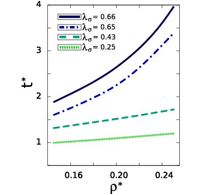
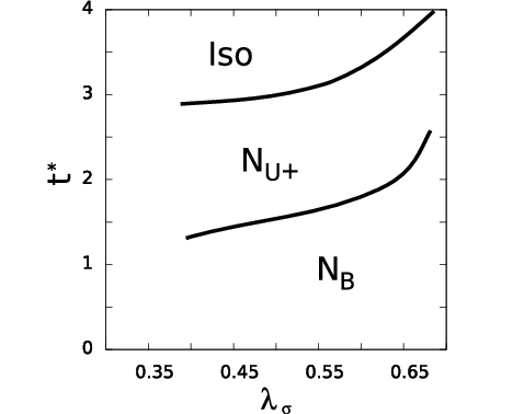
There are some matters which are of interest, and we take them systematically into account. Firstly, there is the question of opposite signs of ${{{{\lambda}}}}_{{{{{\sigma}}}}}$ and ${{{{\lambda}}}}_{{{{{\epsilon}}}}}$ , which was pointed out by Berardi and Zannoni in [35]. Next, we can wonder how the change in the shape or energy biaxiality separately vary the transition temperatures. Then, we can ask ourselves how those two parameters concur in the creation of biaxial nematic, and whether it is possible to induce a Landau point in this model by changing ${{{{\lambda}}}}_{{{{{\epsilon}}}}}$ and ${{{{\lambda}}}}_{{{{{\sigma}}}}}$ , and if so, then how the position of that point changes with the biaxialities. Since we know the relation between axes of biaxial ellipsoids at self-dual point for the models of purely repulsive forces (3.32) (hard molecules [29, 80]), once we find this point in present model, we can estimate the influence of attractive (soft) interaction on its position, but more importantly we can check whether a similar condition is in force for parameters $\{{{{{\sigma}}}}_{i}\}$ and $\{{{{{\epsilon}}}}_{i}\}$ .

Molecular shape effects

Firstly, we take a look at the influence of shape biaxiality on the bifurcation temperature for the rod-like uniaxial to biaxial nematic transition. We change ${{{{\lambda}}}}_{{{{{\sigma}}}}}$ , while keeping $\{{{{{\epsilon}}}}_{i}\}$ fixed, along the path depicted in Fig. 3.10 (thick, gradient line). Figure 3.11(a) represents bifurcation lines in $({{{{\rho}}}}^{*},t^{*})$ plane for different values of ${{{{\lambda}}}}_{{{{{\sigma}}}}}$ , and since we are interested in shape dependence alone, the energy biaxiality ${{{{\lambda}}}}_{{{{{\epsilon}}}}}=0.0$ (for $(d)_{{{{{\epsilon}}}}}$ in Table 3.3). As expected, the increase in the molecular biaxiality leads to higher temperatures for $\textnormal{N}_{U+}$ – $\textnormal{N}_{B}$ transition, chances for observing the biaxial nematic phase are increasing.
Fig. 3.11(b) shows the bifurcation diagram, where temperatures are plotted as function of shape biaxiality both for transition from isotropic phase and for $\textnormal{N}_{U+}$ – $\textnormal{N}_{B}$ case. We can see that the line of uniaxial – biaxial nematic bifurcation gets closer to the $Iso$ – $\textnormal{N}_{U+}$ one, with a prospect of meeting it eventually.

Biaxiality of soft part of the potential

Now we show how the biaxiality stored in $({{{{\epsilon}}}}_{x},{{{{\epsilon}}}}_{y},{{{{\epsilon}}}}_{z})$ affects the transition point. For fixed ${{{{\lambda}}}}_{{{{{\sigma}}}}}$ , we change ${{{{\lambda}}}}_{{{{{\epsilon}}}}}$ by increasing $|{{{{\epsilon}}}}_{x}-{{{{\epsilon}}}}_{y}|$ while keeping ${{{{\epsilon}}}}_{z}=0.2$ . In Fig. 3.12(a) we present bifurcation lines ( $t^{*}$ as function of ${{{{\rho}}}}^{*}$ ) for $\textnormal{N}_{U+}$ – $\textnormal{N}_{B}$ transition, plotted for different values of ${{{{\lambda}}}}_{{{{{\epsilon}}}}}$ and for uniaxial molecule ( ${{{{\lambda}}}}_{{{{{\sigma}}}}}=0.0$ for $(a)_{{{{{\sigma}}}}}$ in Table 3.3). As in the case of Fig. 3.11(a), the dependence of the temperature on density in Fig. 3.12(a) is almost trivial (linear), and is also weaker than in Fig. 3.11(a).
The Figure 3.12(b) shows the bifurcation diagram with isotropic, $\textnormal{N}_{U+}$ , and $\textnormal{N}_{B}$ regions as function of ${{{{\lambda}}}}_{{{{{\epsilon}}}}}$ , for uniaxial shape ${{{{\lambda}}}}_{{{{{\sigma}}}}}=0.0$ for $(a)_{{{{{\sigma}}}}}$ . It can be seen that for low shape biaxialities it is required to supply increasingly high energy biaxiality in order to produce $\textnormal{N}_{B}$ . As was mentioned earlier, ${{{{\lambda}}}}_{{{{{\epsilon}}}}}$ was changed by increasing the difference between ${{{{\epsilon}}}}_{x}$ and ${{{{\epsilon}}}}_{y}$ , and essentially we did not cross the boundary between ”disc-like” and ”rod-like potential” regimes, that is the reason why in Fig. 3.12(b) only prolate nematic phase is observed. Nevertheless, the plot suggests that it is possible for the lines of $Iso$ – $\textnormal{N}_{U+}$ and $\textnormal{N}_{U+}$ – $\textnormal{N}_{B}$ transitions to meet somewhere, for higher energy biaxiality.
From Figures 3.11 and 3.12, we can see that the main factors affecting the diagram are the biaxiality of molecule ${{{{\lambda}}}}_{{{{{\sigma}}}}}$ and the biaxiality of potential ${{{{\lambda}}}}_{{{{{\epsilon}}}}}$ . Thus we can wonder how the combined shape and energy biaxialities influence the bifurcation temperature.

Concurring biaxialities

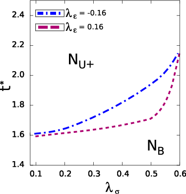
Turning our attention to the question of the influence of both biaxialities, now we allow ${{{{\lambda}}}}_{{{{{\epsilon}}}}}$ and ${{{{\lambda}}}}_{{{{{\sigma}}}}}$ to change simultaneously. It is done as before: shape biaxiality varies along the path in Fig. 3.10, and ${{{{\lambda}}}}_{{{{{\epsilon}}}}}$ by increasing $|{{{{\epsilon}}}}_{x}-{{{{\epsilon}}}}_{y}|$ for ${{{{\epsilon}}}}_{z}=0.2$ . Firstly we consider the case of positive and negative ${{{{\lambda}}}}_{{{{{\epsilon}}}}}$ , while keeping ${{{{\lambda}}}}_{{{{{\sigma}}}}}>0$ . Figure 3.13 shows the bifurcation temperatures as function of shape biaxiality for two cases of ${{{{\lambda}}}}_{{{{{\epsilon}}}}}=-0.16$ and ${{{{\lambda}}}}_{{{{{\epsilon}}}}}=0.16$ , for $\textnormal{N}_{U+}$ – $\textnormal{N}_{B}$ transition. This plot shows the difference between opposite signs of ${{{{\lambda}}}}_{{{{{\sigma}}}}}$ and ${{{{\lambda}}}}_{{{{{\epsilon}}}}}$ . It can be seen that the branch corresponding to negative energy biaxiality is above the positive one almost everywhere, except the point where ${{{{\lambda}}}}_{{{{{\sigma}}}}}=0.0$ (Fig. 3.12(b) is symmetric under the change of sign of ${{{{\lambda}}}}_{{{{{\epsilon}}}}}$ ), and the region where shape biaxiality becomes (relatively to ${{{{\lambda}}}}_{{{{{\epsilon}}}}}$ ) high enough to take control over the transition. A more detailed study on the concurring biaxialities is presented in Figs. 3.14(a)-3.14(b), where the lines of bifurcation for $\textnormal{N}_{U+}$ – $\textnormal{N}_{B}$ transition are plotted as function of ${{{{\lambda}}}}_{{{{{\sigma}}}}}$ for different values of ${{{{\lambda}}}}_{{{{{\epsilon}}}}}$ (Fig. 3.14(a)) and in the opposite case (Fig. 3.14(b)).

Summary of the results can be seen in Figures 3.15 and 3.16, where the surface of bifurcation points is plotted against both the shape and energy biaxialities, in the rod-like and disc-like molecular regime, respectively. The line drawn on the upper surface (representing the transition from isotropic phase to $\textnormal{N}_{U}$ ) in Fig. 3.15 is a family of Landau points where the direct second order transition to biaxial nematic from isotropic liquid phase takes place. Those points will be taken into closer consideration in the following section.

Landau points

Previously, we have seen how the parameters ${{{{\lambda}}}}_{{{{{\epsilon}}}}}$ and ${{{{\lambda}}}}_{{{{{\sigma}}}}}$ , representing the degree of overall biaxiality of the intermolecular potential energy (3.21), influence the bifurcation temperature and density. In present section we will locate the Landau points in $\left({{{{\lambda}}}}_{{{{{\sigma}}}}},{{{{\lambda}}}}_{{{{{\epsilon}}}}}\right)$ space, keeping in mind that ${{{{\lambda}}}}_{{{{{\sigma}}}}}$ is changed along the path drawn with gradient in Fig. 3.10, while in the case of ${{{{\lambda}}}}_{{{{{\epsilon}}}}}$ we hold ${{{{\epsilon}}}}_{z}=0.2$ and starting from ${{{{\lambda}}}}_{{{{{\epsilon}}}}}=0.0$ for ${{{{\epsilon}}}}_{x}={{{{\epsilon}}}}_{y}$ , vary the energy biaxiality by increasing $|{{{{\epsilon}}}}_{x}-{{{{\epsilon}}}}_{y}|$ . We will also comment on the meaning of the hard biaxial ellipsoids self-dual plane $({{{{\lambda}}}}_{{{{{\epsilon}}}}}^{sd},{{{{\lambda}}}}_{{{{{\sigma}}}}}^{sd})$ (3.32)-(3.34), and its relation to Landau points in present model. Firstly, we will investigate uniaxial energy ${{{{\lambda}}}}_{{{{{\epsilon}}}}}=0.0$ ( $(d)_{{{{{\epsilon}}}}}$ in Table 3.3) and look for shape-induced effects, then we will turn to the case of fixed shape biaxiality and by changing ${{{{\lambda}}}}_{{{{{\epsilon}}}}}$ pursuit the Landau point, and finally we will show how both ${{{{\lambda}}}}_{{{{{\epsilon}}}}}$ and ${{{{\lambda}}}}_{{{{{\sigma}}}}}$ change the position of this point on the bifurcation diagram.
In Fig. 3.17(a) we present the bifurcation line as function of shape biaxiality for ${{{{\lambda}}}}_{{{{{\epsilon}}}}}=0.0$ for $(d)_{{{{{\epsilon}}}}}$ . It can be seen that there exists a point at the boundary of disks and rods, where the molecule belongs to neither one of those groups and $\textnormal{N}_{U+}$ and $\textnormal{N}_{U-}$ phases are indistinguishable. This is an isolated Landau point, located near ${{{{\lambda}}}}_{{{{{\sigma}}}}}=0.7163$ for $(g)_{{{{{\sigma}}}}}$ (see Table 3.3). It differs from the predicted for hard biaxial ellipsoids [29, 80] self-dual geometry ${{{{\sigma}}}}_{x}=\sqrt{{{{{\sigma}}}}_{y}{{{{\sigma}}}}_{z}}$ (3.32), which in our parametrization would be at ${{{{\lambda}}}}_{{{{{\sigma}}}}}=0.6412$ for $(c)_{{{{{\sigma}}}}}$ . As we can see, the attractive forces shift the position of Landau point towards higher values of ${{{{\lambda}}}}_{{{{{\sigma}}}}}$ .
If we can induce the transition directly to biaxial nematic phase by changing ${{{{\lambda}}}}_{{{{{\sigma}}}}}$ , then it should be possible to do the same thing for ${{{{\lambda}}}}_{{{{{\epsilon}}}}}$ . Figure 3.17(b) shows such bifurcation diagram as function of energy biaxiality for ${{{{\lambda}}}}_{{{{{\sigma}}}}}=0.70$ for $(f)_{{{{{\sigma}}}}}$ . It is clear that for ${{{{\lambda}}}}_{{{{{\sigma}}}}}\neq 0$ by changing ${{{{\lambda}}}}_{{{{{\epsilon}}}}}$ we can induce a Landau point. We should recall, however, that we do not cross the boundary between ”rod-like” and ”disc-like” energies (in terms of $({{{{\epsilon}}}}_{x},{{{{\epsilon}}}}_{y},{{{{\epsilon}}}}_{z})$ or ${{{{\lambda}}}}_{{{{{\epsilon}}}}}$ ). It turns out that for shape biaxialities close to the ones giving Landau point by strengthening the lateral interactions we can also induce a self-dual point (e.g. the left one in Fig. 3.17(b)).

Plot presented in Figure 3.17(b) gives us also some insight into the issue of dependence of Landau point position on ${{{{\lambda}}}}_{{{{{\epsilon}}}}}$ and ${{{{\lambda}}}}_{{{{{\sigma}}}}}$ . There exist two such points in Fig. 3.17(b) for ${{{{\lambda}}}}_{{{{{\sigma}}}}}=0.70$ whereas in Fig. 3.17(a) for a bit higher shape biaxiality ${{{{\lambda}}}}_{{{{{\sigma}}}}}=0.7163$ there is only one Landau point visible. Given all this we can wonder how the location of this point changes under the varying biaxialities. We can plot Landau point position and divide the $\left({{{{\lambda}}}}_{{{{{\sigma}}}}},\,{{{{\lambda}}}}_{{{{{\epsilon}}}}}\right)$ space into disc and rod-like regions, as is shown in Figure 3.18, while keeping in mind the way $({{{{\sigma}}}}_{x},{{{{\sigma}}}}_{y},{{{{\sigma}}}}_{z})$ and $({{{{\epsilon}}}}_{x},{{{{\epsilon}}}}_{y},{{{{\epsilon}}}}_{z})$ were changed and combined into ${{{{\lambda}}}}_{{{{{\sigma}}}}}$ and ${{{{\lambda}}}}_{{{{{\epsilon}}}}}$ . It can be seen that it is ”easier” to procure a transition directly to biaxial nematic phase for the case of the same sign of ${{{{\lambda}}}}_{{{{{\sigma}}}}}$ and ${{{{\lambda}}}}_{{{{{\epsilon}}}}}$ , whereas in the case of negative ${{{{\lambda}}}}_{{{{{\epsilon}}}}}$ it takes stronger (relatively to ${{{{\lambda}}}}_{{{{{\sigma}}}}}$ ) energy biaxialities to induce a Landau point. The increase of ${{{{\lambda}}}}_{{{{{\sigma}}}}}$ resulted in meeting of the two Landau points visible on Fig. 3.17(b) at a single point for $\left({{{{\lambda}}}}_{{{{{\sigma}}}}},{{{{\lambda}}}}_{{{{{\epsilon}}}}}\right)=\left(0.7163,0.0\right)$ as presented in Fig. 3.17(a).

More interestingly, we can make some comments on the meaning of the self-dual condition for hard, biaxial ellipsoids (3.32)-(3.34). We can see that it is possible to find Landau point away from the square root plane $({{{{\lambda}}}}_{{{{{\epsilon}}}}}^{sd},{{{{\lambda}}}}_{{{{{\sigma}}}}}^{sd})$ (3.33)-(3.34), it is visible in Fig. 3.17(a). We have also investigated vicinity of the point lying in this plane at $({{{{\lambda}}}}_{{{{{\epsilon}}}}}^{sd},{{{{\lambda}}}}_{{{{{\sigma}}}}}^{sd})=(0.175,0.6412)$ ( $(h)_{{{{{\epsilon}}}}}$ and $(c)_{{{{{\sigma}}}}}$ in Table 3.3) and found the Landau point at $({{{{\lambda}}}}_{{{{{\epsilon}}}}},{{{{\lambda}}}}_{{{{{\sigma}}}}})=(0.175,0.6596)$ ( $(h)_{{{{{\epsilon}}}}}$ and $(d)_{{{{{\sigma}}}}}$ ). We can conclude, although based only on the four points (lying on the upper line in Fig. 3.18), that square root rule (3.32) is a good candidate for the starting position in the search for Landau points; we have shown that self-dual points can exist beyond $({{{{\lambda}}}}_{{{{{\epsilon}}}}}^{sd},{{{{\lambda}}}}_{{{{{\sigma}}}}}^{sd})$ plane, but also in its vicinity. As we can see, the upper line in Fig. 3.18 crosses the vicinity of the point on the plane in $({{{{\lambda}}}}_{{{{{\epsilon}}}}},{{{{\lambda}}}}_{{{{{\sigma}}}}})$ space defined by square root rule. When we consider the complicated, non-linear manner in which $\{{{{{\epsilon}}}}_{i}\}$ and $\{{{{{\sigma}}}}_{i}\}$ contribute to the biaxial Gay-Berne potential, it is surprising that the Landau points can be found close to the plane obtained from the simple square root rule: ${{{{\epsilon}}}}_{x}=\sqrt{{{{{\epsilon}}}}_{y}{{{{\epsilon}}}}_{z}}$ , ${{{{\sigma}}}}_{x}=\sqrt{{{{{\sigma}}}}_{y}{{{{\sigma}}}}_{z}}$ .

The bifurcation analysis can give the position of Landau point (using Eq. (2.72)); however, in its vicinity it becomes increasingly hard to stabilize the uniaxial nematic reference phase because it looses stability at this point. Therefore, in order to confirm the places where self-dual point appears to exist, we have employed the method of minimisation of the Helmholtz free energy (3.5) with trial one-particle distribution function (3.9) by solving the equations (3.10) and obtained the temperature and density of the transition by calculating order parameters (2.49). An example of the behaviour of the leading order parameters at the Landau point is presented in Fig. 3.19, and for comparison we also show the plots away from this point in rod-like regime, both obtained from the minimisation method.

3.4.5 Summary

The uniaxial Gay-Berne potential [96, 97] achieved an amazing, compared to its simplicity, success in predicting liquid crystal phase behaviour. As pointed out before, most of the mesogenic molecules are not uniaxial. They are not biaxial either, but effectively in the uniaxial phase they can be approximated by ellipsoids of revolution, as was done in the original Gay-Berne interaction, and in biaxial phase by $D_{2h}$ – symmetric objects, as in the potential developed by Berardi, Fava and Zannoni [36]. We have investigated the latter model.

We compared the bifurcation analysis of DFT in low-density approximation with the Monte Carlo results. As expected the bifurcation temperatures were significantly higher than those following from simulations. This tendency was more apparent in case for $Iso$ – $\textnormal{N}_{U+}$ transition, while for $\textnormal{N}_{U+}$ – $\textnormal{N}_{B}$ bifurcation the approach provided more accurate estimates in relation to Monte Carlo. The comparison was only qualitative because the simulation study neglected long-range corrections, the inclusion of which makes the results of Monte Carlo closer to those of DFT [108].
Then, in order to provide some insight into the way the reference state influences the phase diagram, we calculated the bifurcation for $\textnormal{N}_{U+}$ – $\textnormal{N}_{B}$ transition using the minimisation of the Helmholtz free energy. This method does not involve the truncation of the expansion of the pair direct correlation, but uses the whole function, and therefore, compared to bifurcation for second order phase transition, provides the estimation of the influence of precisely calculated one-particle distribution function of reference phase. The results show that the inclusion of terms with higher angular momentum index than $2$ in the expansion of pair direct correlation function has secondary meaning.

Next, we continued to investigate the influence of introduced earlier shape biaxiality ${{{{\lambda}}}}_{{{{{\sigma}}}}}$ and energy biaxiality ${{{{\lambda}}}}_{{{{{\epsilon}}}}}$ on the bifurcation diagram, by defining a path in the six dimensional space of potential shape and energy parameters. We presented the diagrams for uniaxial cases of the potential ( ${{{{\lambda}}}}_{{{{{\epsilon}}}}}=0.0$ ) for different values of the biaxiality of shape, and uniaxial shape ( ${{{{\lambda}}}}_{{{{{\sigma}}}}}=0.0$ ) was studied for given energy biaxialities. We also addressed the issue of opposite signs of ${{{{\lambda}}}}_{{{{{\sigma}}}}}$ and ${{{{\lambda}}}}_{{{{{\epsilon}}}}}$ . With increasing positive ${{{{\lambda}}}}_{{{{{\sigma}}}}}$ , for uniaxial – biaxial nematic bifurcation the line of transitions corresponding to ${{{{\lambda}}}}_{{{{{\epsilon}}}}}<0$ was lying in temperatures higher than the one associated with ${{{{\lambda}}}}_{{{{{\epsilon}}}}}>0$ , apart from the point when ${{{{\lambda}}}}_{{{{{\sigma}}}}}$ became large enough to dominate the transition. The results showed how the $\textnormal{N}_{U}$ – $\textnormal{N}_{B}$ transition is influenced by the Gay-Berne interaction biaxiality originating from different sources. They also suggested that the model can exhibit a Landau point; this possibility was also investigated.
We found that by increasing ${{{{\lambda}}}}_{{{{{\sigma}}}}}$ for ${{{{\lambda}}}}_{{{{{\epsilon}}}}}=0.0$ we can cross the boundary between the oblate and prolate nematic phases and locate the Landau point when the distinction between them is not possible, where $Iso$ , $\textnormal{N}_{U-}$ , $\textnormal{N}_{U+}$ , and $\textnormal{N}_{B}$ phases ”meet”, and the second order isotropic – biaxial nematic phase transition occurs. This shape-induced self-dual point was found to be located at higher shape biaxiality than the one obtained for hard molecules. In terms of ${{{{\lambda}}}}_{{{{{\sigma}}}}}$ , the difference between the shape biaxiality at Landau point following from our analysis (with ${{{{\lambda}}}}_{{{{{\epsilon}}}}}=0.0$ , so the biaxiality of the interaction originated only in shape of molecules), and the one obtained for hard biaxial ellipsoids was found to be $0.0751$ . This difference is the estimate of the degree of the influence of attractive, anisotropic forces on Landau point position. The self-dual points were also found to occur for fixed shape biaxiality when ${{{{\lambda}}}}_{{{{{\epsilon}}}}}$ was changed. In this case we varied the energy biaxiality by going from the model of strong lateral interactions to the one where molecules are most attracted to their faces (we did not cross the ”rod-like” and ”disc-like potential” boundary in terms of ${{{{\lambda}}}}_{{{{{\epsilon}}}}}$ ). When energy parameters fulfilled the self-dual square root rule for hard ellipsoids, the Landau point was found for the ${{{{\lambda}}}}_{{{{{\sigma}}}}}$ different from the one predicted for hard potentials by $0.0184$ . The same difference, far away from ${{{{\epsilon}}}}_{x}=\sqrt{{{{{\epsilon}}}}_{y}{{{{\epsilon}}}}_{z}}$ , for ${{{{\lambda}}}}_{{{{{\epsilon}}}}}=0.0$ was more than four times higher. The matter requires further studies, but our results suggest that the meaning of the square root rule maintains its importance as the qualitatively accurate estimates for Landau region for soft biaxial Gay-Berne interaction. We concluded our findings by the division of $({{{{\lambda}}}}_{{{{{\epsilon}}}}},{{{{\lambda}}}}_{{{{{\sigma}}}}})$ space into regions belonging to the oblate and prolate states. It proved that the line of Landau points crosses the vicinity of the point following from square root rule for $\{{{{{\epsilon}}}}_{i}\}$ and $\{{{{{\sigma}}}}_{i}\}$ . The existence of Landau points their position and order of the transition were confirmed by the minimisation of the Helmholtz free energy.
The thermotropic biaxial nematic phase discovered in simulations by Berardi and Zannoni was reported for the model of stronger lateral interactions, i.e., where the side-to-side configuration is preferred (see Fig. 3.5), that is, for opposite signs of shape and energy biaxiality. Our results suggest that while the temperature of $\textnormal{N}_{U+}$ – $\textnormal{N}_{B}$ transition is relatively higher for negative ${{{{\lambda}}}}_{{{{{\epsilon}}}}}$ (while ${{{{\lambda}}}}_{{{{{\sigma}}}}}$ is greater than zero, see Fig. 3.13) it is necessary to provide significantly lower (negative) energy biaxialities to induce the Landau point in that case (see Fig. 3.18). Whereas for positive biaxialities the transition directly to biaxial nematic can occur for moderate values of ${{{{\lambda}}}}_{{{{{\epsilon}}}}}$ and ${{{{\lambda}}}}_{{{{{\sigma}}}}}$ . We shed some light on the issue of the case ${{{{\lambda}}}}_{{{{{\sigma}}}}}>0$ , ${{{{\lambda}}}}_{{{{{\epsilon}}}}}<0$ in the last chapter, where we take into account uniaxial and biaxial smectic-A phases; it is natural to suspect that those structures are preferred over $\textnormal{N}_{B}$ when the interaction favours face-to-face configuration over side-to-side.

Apparently, in case of biaxial nematic, the significance of the Gay-Berne interaction is much smaller than for uniaxial phases. Therefore, in order to continue the search for factors behind the stabilisation of $\textnormal{N}_{B}$ , we need to study a model that can be more closely related to the real systems. We turn our attention to the bent-core molecules.

3.5 Systems of bent-core molecules

In present section we consider the models of bent-core (banana) molecules built from Gay-Berne segments³³ 3 Which is a simple way to do it, but at least guarantees the basic correct behaviour of the molecule.. We study shape-related effects and the influence of dipole-dipole interaction. Firstly, we take into account the case of $D_{\infty h}$ – symmetric arms and join two and three prolate, soft ellipsoids, as presented in Fig. 3.20, to model banana-like molecules with bend (opening) angle ${{{{\gamma}}}}$ . The system is studied for fixed density, and the resulting bifurcation diagrams are presented in the plane of temperature $t^{*}$ (see (3.20)) and ${{{{\gamma}}}}$ . We especially focus on Landau point position, as obtained from (2.72), and in order to shed more light on this issue, we also take a look at the behaviour of Landau region when the arms deviate from $D_{\infty h}$ symmetry; we incorporate two soft, biaxial ellipsoids into a bent-core molecule using the Berardi-Fava-Zannoni potential [36], studied in the previous section. Inspired by recent developments [46], we also comment on the asymmetric bent-core molecules with arms modelled by soft, $D_{\infty h}$ – symmetric ellipsoids of different elongations, using potential from [103]. Finally, we turn to the effects of polarity, and we include dipole-dipole interaction between the dipole moments located along $C_{2}$ symmetry axis of the molecule (see Fig. 3.20). We present the phase diagrams in $(t^{*},{{{{\gamma}}}})$ plane for fixed density at bifurcation point, again focusing on the behaviour of Landau point.
We begin with a description of the model, then we present the bifurcation diagrams for non-polar case for uniaxial and biaxial arms, and then we study the influence of dipole-dipole interaction.

3.5.1 Models of a bent-core molecule

This section is devoted to the description of the pair potential that was used as an interaction between two bent-core molecules. We are using two already mentioned models, those are: the uniaxial Gay-Berne [96, 97] and its biaxial version as proposed by Berardi, Fava, and Zannoni [35]. Fig. 3.20 shows the construction. Each of the parts interacts with every one on the other banana, while the interaction between segments within single molecule, giving an irrelevant constant, is disregarded. We consider rigid bananas, i.e., we do not allow the change of the angle ${{{{\gamma}}}}$ or dimensions of the ellipsoids during the calculations.

The intermolecular potential can be written as (see Fig. 3.20):

\begin{split}V_{b2}=&\sum_{a,b\in\left\{1,2\right\}}V_{GB}\left({{\mathbf{\hat{u}}}}_{1,a},{{\mathbf{\hat{u}}}}_{2,b},\vec{\mathbf{r}}_{ab}\right)\,,\\ V_{b3}=&\sum_{a,b\in\left\{1,2,3\right\}}V_{GB}\left({{\mathbf{\hat{u}}}}_{1,a},{{\mathbf{\hat{u}}}}_{2,b},\vec{\mathbf{r}}_{ab}\right)\,,\end{split}

(3.35)

where, as before, $V_{GB}$ is either the uniaxial Gay-Berne potential, described in Sec. 3.4.1, or its biaxial version studied in previous section and introduced in Sec. 3.4.2, ${{\mathbf{\hat{u}}}}_{i,j},\,(i=1\dots 2,\,j=1\dots 3)$ are unit vectors parallel to the Gay-Berne segments symmetry axes, $\vec{\mathbf{r}}_{ij}$ are vectors connecting the centres of molecules. For $D_{2h}$ – symmetric Gay-Berne, in order to describe the orientation of the ellipsoid, it is not enough to give the vector parallel to the longer axis, in this case we fixed the remaining axes with respect to the plane of the angle ${{{{\gamma}}}}$ , namely one axis was set to lie in this plane and the other to be perpendicular to it. For the uniaxial Gay-Berne the empirical exponents $\tilde{{{{{\nu}}}}}$ , $\tilde{{{{{\mu}}}}}$ are chosen to be to $1$ and $2$ , respectively, and the elongation of the ellipsoids is $5:1$ , and anisotropy of the potential $4:1$ , in terms of constants from (3.16) and Eq. (3.19) it means ${{{{\kappa}}}}=5$ and ${{{{\chi}}}}^{{}^{\prime}}=1/3$ (see Fig. 3.4(b)). The molecular elongations are chosen to correspond to the dimensions of the bent-core compounds.
We have also added the dipole moment localized in the fixed position, as shown in Fig. 3.20, along molecular $C_{2}$ symmetry axis. The dipole-dipole interaction used is of a well known form:

V_{DD}\left(\vec{\mathbf{\mbox{\boldmath{${{{{\mu}}}}$}}}}_{1},\vec{\mathbf{\mbox{\boldmath{${{{{\mu}}}}$}}}}_{2},\vec{\mathbf{r}}\,\right)=\frac{\vec{\mathbf{\mbox{\boldmath{${{{{\mu}}}}$}}}}_{1}\cdot\vec{\mathbf{\mbox{\boldmath{${{{{\mu}}}}$}}}}_{2}-3\left(\vec{\mathbf{\mbox{\boldmath{${{{{\mu}}}}$}}}}_{1}\cdot{{\mathbf{\hat{r}}}}\right)\left(\vec{\mathbf{\mbox{\boldmath{${{{{\mu}}}}$}}}}_{2}\cdot{{\mathbf{\hat{r}}}}\right)}{r^{3}}\,,

where $\vec{\mathbf{\mbox{\boldmath{${{{{\mu}}}}$}}}}_{i}={{{{\mu}}}}^{*}{{\mathbf{\hat{\mbox{\boldmath{${{{{\mu}}}}$}}}}}}_{i}$ , and where ${{\mathbf{\hat{\mbox{\boldmath{${{{{\mu}}}}$}}}}}}_{i}$ is a unit vector, and ${{{{\mu}}}}^{*}$ is the dimensionless (see (3.20)) magnitude of the dipole moment. To provide some way of relating ${{{{\mu}}}}^{*}$ to the strength of $V_{GB}$ , we have calculated $\left|\frac{V_{DD}}{V_{b3}+V_{DD}}\right|$ in the ground state for given values of ${{{{\mu}}}}^{*}$ (see Table 3.4). This ratio gives relative weight of contribution from dipole-dipole interaction to total potential; it will be used as a measure of dipole strength.
We employ the units of energy ( ${{{{\epsilon}}}}_{0}$ ) and distance ( ${{{{\sigma}}}}_{0}$ ) as described by (3.20). Results presented in this section follow from using in place of $V$ in Eq. (3.1)-(3.2) $V_{b2}$ or $V_{b3}$ , with $V_{DD}$ added in polar case.

Table 3.4: Dipole-dipole interaction contribution to total potential energy in the ground state.

${{{{\mu}}}}^{*}$	$\left\|V_{DD}/\left(V_{b3}+V_{DD}\right)\right\|$
$2.8$	$0.50$
$2.2$	$0.40$
$1.6$	$0.25$
$1.5$	$0.22$
$1.2$	$0.15$

The absolute minimum of the potential between two banana-like molecules (the ground state) for the non-polar uniaxial model corresponds to the configuration where ${{{\mathbf{\hat{b}}}}}^{1}_{i}$ and ${{{\mathbf{\hat{b}}}}}^{2}_{i}$ axes of frames associated with molecule $1$ and $2$ (see Fig. 3.20) are parallel and the vector $\vec{\mathbf{r}}$ is oriented along ${{\mathbf{\hat{b}}}}^{1}_{1}$ . The inclusion of the dipole-dipole interaction changes that picture; in the ground state relative orientation is the same, only $\vec{\mathbf{r}}$ is parallel to ${{\mathbf{\hat{b}}}}^{1}_{2}$ .

In numerical analysis for two-part banana, to prevent the infinite values of potential when dipoles are localized at the same point, we have introduced a hard sphere between the arms with radius of $0.5\,{{{{\sigma}}}}_{0}$ . Fig. 3.21 (not containing the just-mentioned sphere) shows the equipotential surfaces for the model where uniaxial Gay-Berne potential was used, for four relative orientations of two molecules.
Every bifurcation diagram presented in this chapter was calculated at fixed density chosen in the following way. If we calculate the inverse of the excluded volume for parallel bent-core molecules we will receive values of $0.024\,{{{{\sigma}}}}^{-3}_{0}$ and $0.016\,{{{{\sigma}}}}^{-3}_{0}$ for two, and three -arm bananas, respectively. The densities on the diagrams were set to be of that order, which corresponds to packing fractions (molecular volume per average volume of molecule) of $0.2$ and $0.3$ , being slightly lower than typical values in uniaxial nematic which range from $0.4$ to $0.6$ .
In the following section we present the bifurcation diagrams for bent-core molecules without dipole moments.

3.5.2 Shape-induced effects

In present section we seek the answer for the most straight forward question of what happens to the bifurcation temperature as we change the opening angle ${{{{\gamma}}}}$ , and also whether we can find Landau points, where direct transition from the isotropic to biaxial nematic phase takes place. Since we pursuit only the shape related effects, we do not introduce any dipole-dipole interactions yet. Firstly, we present the results for model where the arms of bent-core molecule are uniaxial ellipsoids of revolution, and then we take a brief look at the case of $D_{2h}$ – symmetric building blocks.

Uniaxial arms

We can think of the arms of a banana (see Fig. 1.13) as of uniaxial ellipsoids. This approximation probably will not reflect all properties of the bent-core molecule correctly, but can serve as a starting point for more complex models.

Table 3.5: Temperatures of bifurcation from isotropic phase for

{{{{\gamma}}}}=90^{\circ}

Model	${{{{\rho}}}}^{*}$	$t^{*}_{90}$
two-arms bent-core molecule	$0.04$	$0.84$
two-arms bent-core molecule	$0.06$	$0.96$
three-arms bent-core molecule	$0.026$	$1.34$
three-arms bent-core molecule	$0.04$	$1.71$

We have taken into account the molecules composed of two and three Gay-Berne interacting parts. In Fig. 3.22 we show the resulting bifurcation diagrams for non-polar banana for two densities. As can be seen, the opening angle at Landau point, for which the direct transition from isotropic phase to the biaxial nematic takes place, for two-part banana is equal to $107^{\circ}$ , which is in agreement with the results for hard interactions [38] and close to the mean field predictions ( $109^{\circ}$ ) [39]. Interestingly, for bent-core molecules composed of two parts the correction to the position of the self-dual point from attractive forces is vanishingly small. We remember that it was not the case for convex biaxial molecules (see Fig. 3.17(a)). The model of three arms, as is shown on Fig. 3.22(b), has the Landau point localized near the right angle, which can be considered to be in some agreement with observations in [61], where the mesogenic substance consisting of molecules with bend angle of $90^{\circ}$ was found to give rise to biaxial nematic phase. The summary of Landau points positions is presented in Table 3.6.
In order to pursuit the behaviour of Landau point in the two-arm model, we have also taken into account asymmetrical bananas, i.e., we constructed the bent-core molecules from two uniaxial ellipsoids with different elongations. We used the extended Gay-Berne potential [103] and performed the calculations for a range of asymmetries, up to a point where one arm was four times longer than the other. No significant differences in the position of the Landau point were found, it was located, as for symmetric bananas, at $107^{\circ}$ .
Non-polar model of uniaxial arms is able to produce an isolated self-dual point, given in Table 3.6. Following sections show two models where that behaviour is different, namely, there appears a line of Landau points.

Bent-core systems composed of biaxial parts

It is of interest to take into account the model where the arms of a banana are not uniaxial. One possibility would be to consider the bent-core molecules built of the biaxial parts. We have done so, and present the resulting phase diagram in current section.

Table 3.6: Landau point position versus strength of the dipole

{{{{\mu}}}}^{*}

Bent-core model	${{{{\mu}}}}^{*}$	opening angle at Landau point
two-arms	$0.0$	$107^{\circ}$
	$1.2$	$104^{\circ}$
	$1.5$	$103^{\circ}$
three-arms		${{{{\rho}}}}^{}=0.026$ $\,\,{{{{\rho}}}}^{}=0.04$
	$0.0$	$\,\,\,89^{\circ}$ $\,89^{\circ}$
	$1.2$	$\,\,\,86^{\circ}$ $\,86^{\circ}$
	$1.6$	$\,\,\,74^{\circ}$ - $86^{\circ}$ $\,74^{\circ}$ - $86^{\circ}$
	$2.0$	$\,\,\,63^{\circ}$ - $86^{\circ}$ $\,63^{\circ}$ - $80^{\circ}$
	$2.8$	$\,\,\,83^{\circ}$ - $97^{\circ}$ $\,82^{\circ}$ - $92^{\circ}$
two biaxial arms	$0.0$	$121^{\circ}$ - $128^{\circ}$

We take the biaxial Gay-Berne ellipsoids as building blocks. They are oriented in the following way. We fix the plane of the longer axis, to lie in the plane of the bend angle, while the shortest axis is chosen to be perpendicular to it. In this way we construct the bent-core molecule as shown in Fig. 3.20, and build the pair interaction by substituting $V_{GB}$ in (3.35) with the biaxial Gay-Berne potential (3.21), defined in Sec. 3.4.2. The resulting pair interaction has the global minimum in the same configuration as the uniaxial two-arm model described in the previous subsection.
We are mainly interested in the position of the Landau point in this model. We have chosen the shape of constituting biaxial ellipsoids to be $\left({{{{\sigma}}}}_{x},{{{{\sigma}}}}_{y},{{{{\sigma}}}}_{z}\right)=\left(1.2,0.514,3.4\right)$ and the potential parameters $\left({{{{\epsilon}}}}_{x},{{{{\epsilon}}}}_{y},{{{{\epsilon}}}}_{z}\right)=\left(1.0,1.4,0.2\right)$ . As mentioned in the previous chapter those parameters make the attractive forces strongest in the face-to-face configuration, that is, in the direction of the shortest axis (see Sec. 3.4.2). This model exhibits molecular biaxiality in the limit of ${{{{\gamma}}}}={{{{\pi}}}}$ and ${{{{\gamma}}}}=0$ ; however, it is as well clear that there should exist an angle for which Landau point appears. Indeed, the numerical analysis shows the existence of self-dual region, in the form of the line of Landau points, as can be seen from Fig. 3.23. For the biaxial arms interacting by biaxial Gay-Berne potential a line of $Iso$ – $\textnormal{N}_{B}$ transitions is possible. It starts near ${{{{\gamma}}}}=121^{\circ}$ and ends for ${{{{\gamma}}}}=128^{\circ}$ , and reduces to a single point with a decrease in arms biaxiality.

The matter should probably be investigated further, since the Landau region obtained for the model with biaxial arms is closer to the experimental findings, not to mention that the topology of the diagram is qualitatively different from what was published in the literature so far.

3.5.3 Polar case

As was mentioned before, molecules studied in [57, 58, 61], i.e., those for which the biaxial nematic was observed, are polar. Therefore, it is interesting to look at the effects of dipole-dipole interaction on stability of the biaxial nematic phase in model bent-core systems. We have introduced the dipole moment along the molecular $C_{2}$ symmetry axis, as depicted in Fig. 3.20. In current section we present the bifurcation diagrams for two and three uniaxial arm models for a couple of dipole strengths. We again focus on the dependence of Landau point position on the dipole magnitude (see Table 3.6).
Fig. 3.24 shows the bifurcation diagrams. As can be seen (Table 3.6) the inclusion of the dipole-dipole interaction shifts the Landau point for the model of two uniaxial arms towards lower angles (Fig. 3.24(a)). In case of bent-core molecule modelled by three uniaxial Gay-Berne parts (Fig. 3.24(b)), for values of dipole strength less than $20\%$ of the total potential in the ground state (see Table 3.4), the same tendency is maintained, i.e., Landau point is shifted towards lower angles up to a value of $86^{\circ}$ . However, for dipoles above ${{{{\mu}}}}^{*}=1.4$ ( $20\%$ of total potential) isolated Landau point changes into the second order $Iso$ – $\textnormal{N}_{B}$ phase transition line. The range of this line measured in opening angles widens; for ${{{{\mu}}}}^{*}=1.6$ it is $12^{\circ}$ and for ${{{{\mu}}}}^{*}=2.0$ exceeds $20^{\circ}$ . For moderate density, its upper limit does not change and is at ${{{{\gamma}}}}=86^{\circ}$ as long as the dipole strength ${{{{\mu}}}}^{*}\leq 2.1$ ( $38\%$ of total energy). Then, the Landau region begins to shrink and is shifted towards higher angles. The highest dipole studied is the one of ${{{{\mu}}}}^{*}=2.8$ for which $V_{DD}$ is $50\%$ of total potential. As can be seen from Fig. 3.24(b), the line of $Iso$ – $\textnormal{N}_{B}$ transitions in that case is still getting shorter, and moves in the direction of higher angles. Fig. 3.25 shows the evolution of Landau region for varying dipole-dipole potential contribution to total energy. When $V_{DD}$ contribution is more than $35\%$ and less than $38\%$ , the Landau line attains its maximal width in opening angle.
We have presented the diagrams for two densities selected from lower region, as described above. It can be seen (Table 3.6) that for strongest dipoles studied ( ${{{{\mu}}}}^{*}\geq 2.0$ ) some differences appear with varying density. Namely, the line of direct isotropic – biaxial nematic transitions gets shorter for higher density.
Our results suggest that there exists a certain range of dipole strength which makes the appearance of biaxial nematic phase most probable. Based on the diagrams presented in Fig. 3.24, and the assumed model parameters, we estimated this region to be between ${{{{\mu}}}}^{*}=1.4$ and $2.1$ , that is, when dipole-dipole interaction contributes in range of $20$ and $38\%$ to total potential energy.
Finally, we should mention that the only other studies in this direction are Monte Carlo simulations of lattice Lebwohl-Lasher model presented in [48], where the introduction of dipoles resulted in the line of direct isotropic – biaxial nematic transitions.

3.5.4 Conclusions

We studied the bent-core molecule model. Firstly, we took into account the bananas composed of two and three uniaxial Gay-Berne ellipsoids. We discussed briefly the case where arms of the molecules interact via biaxial Gay-Berne potential, and also where one arm is a longer uniaxial ellipsoid than the other. The dipole-dipole interactions were introduced next, and the influence of the dipole strength on position of Landau point was studied. Our results qualitatively support the previous findings [38, 39], and show similar behaviour as the less realistic polar, lattice model [48].
The bent-core Gay-Berne model of two uniaxial arms exhibits the Landau point in agreement with previous studies for hard bananas in Onsager approximation and mean field [38, 39]. Its position was not changed significantly by the introduction of attractive forces, nor by the inclusion of anisotropy of the molecule. In case of the three $D_{\infty h}$ – symmetric arms, opening angle near the right angle was distinguished as the one where Landau point appears. Recent experimental studies [61] are in line with these findings.
We tried to address the problem of disagreement between the experimental estimates of the opening angle in the biaxial nematic phase (predicted to be near $140^{\circ}$ ) and the theoretical results by switching to biaxial arms interacting via biaxial Gay-Berne potential. In that model with the increase of arms biaxiality, Landau point evolved to the line of direct $Iso$ – $\textnormal{N}_{B}$ second order phase transitions in range of opening angle ${{{{\gamma}}}}$ between $121^{\circ}$ and $128^{\circ}$ . Probably, inclusion of dipoles or increase in the arms biaxiality or taking into account molecular flexibility could widen that region and possibly shift it towards higher angles.
That behaviour was not possible to acquire in non-polar case of uniaxial arms. The line of direct $Iso$ – $\textnormal{N}_{B}$ transitions appeared in the model of three-part banana with dipole localized along the $C_{2}$ symmetry axis. It appeared that it is possible to provide dipoles strong enough to generate the line of Landau points, which widened with the increase of the dipole strength up to its maximal range in the opening angle ( $63^{\circ}<{{{{\gamma}}}}<86^{\circ}$ ), when the dipole-dipole interaction constituted between $35$ and $38\%$ of total potential. Stronger dipoles began to shrink that line and move it towards higher angles. That should provide some hints for future research. Possibly a study on the orientation of the dipole as well as on the shape of arms and shape of potential is in order, for instance, we could wonder what would happen when shape of arms is close to the self-dual geometry (found in Sec. 3.4.4).

Our studies clearly indicate that strong dipoles were a necessary feature for experimental discovery of the biaxial nematic phase in bent-core systems. In polar case we saw that the dipole-dipole interactions not only were able to shift the position of the Landau point (move it towards lower angles) but also change the topology of the bifurcation diagram to include the self-dual line of direct isotropic – $\textnormal{N}_{B}$ transitions. We can speculate that if the similar mechanism is at work in the substances where the biaxial nematic was observed, then the dipoles indeed became crucial, not only increasing the biaxiality of a molecule but also shifting the $\textnormal{N}_{B}$ region to lower angles where the realization and observation of the elusive phase becomes possible.
We were unable to account for the experimentally predicted value of the opening angle of $140^{\circ}$ , as observed in the first class of the bent-core biaxial materials. The stability of the biaxial nematic for the angles of this magnitude, in comparison to $Iso$ and $\textnormal{N}_{U}$ phases, was very low. The introduction of dipole-dipole interaction shifted the Landau point in the opposite direction, so probably it is safe to conclude that the polarity alone cannot explain the disagreement between theoretical and experimental results. Only the inclusion of biaxial arms interacting via biaxial Gay-Berne potential gave the values of opening angle somewhat closer to $140^{\circ}$ .

Chapter 4 Preliminary results

The knowledge of phase diagram does not give the complete information about behaviour of a system, e.g., from the knowledge of the density-temperature region of stability of a given structure we cannot extract the information about response of a system to a given deformation of the director field. For many applications this kind of information is crucial. This chapter is devoted to the two issues that were disregarded in the preceding part of this thesis. One of them is the investigation of a phenomena related to small distortions of the homeotropic biaxial nematic phase and description of such state in terms of the biaxial elastic constants. The other is the matter of spatially non-uniform liquid crystal states. Presently we show the preliminary results concerning those issues.

4.1 Biaxial elastic constants

Response of the biaxial nematic state to a small perturbations is usually described by the contribution to the free energy coming from the distortion of the directors, expanded in terms of their gradients. The coefficients of this expansion are called elastic constants, and are of great importance to both theoretical and experimental studies. They influence most of the observed phenomena in liquid crystals. To name only a few, we can mention their role in light scattering effects, response to external fields [64], shape of disclination defects [109], and nematodynamic flow [110]. The elastic constants are crucial quantities in applications of liquid crystals in displays [111], and also are of importance in polymer-dispersed systems [112]. They are as well significant for the stability of the thermotropic biaxial nematic phase. The low relative magnitude of elastic constants corresponding to the biaxial distortions in comparison to uniaxial ones can be one of the reasons for difficulties in stabilizing $\textnormal{N}_{B}$ .
The usual way of approaching the issues of elasticity is to study the elastic free energy density dependence on the local deformations. The first derivation is due to Oseen [113], later phenomenologically acquired by Frank [109], and also by Zocher [114]. In those classic papers the liquid is studied by means of the director field ${{\mathbf{\hat{n}}}}(\vec{\mathbf{r}})$ and the deformations of this field give rise to the increase of free energy¹¹ 1 At the level of the molecular interpretation the free energy density of the small elastic deformations is always positive., typically described by expansion in gradients of ${{\mathbf{\hat{n}}}}$ . In the case of biaxial nematic phase, we have two additional directors denoted by ${{\mathbf{\hat{m}}}}$ and ${{\mathbf{\hat{l}}}}$ which are not independent on each other and on the uniaxial director. The fact that the directors form an orthogonal tripod means that we cannot perform an independent distortion of one director field without affecting other two. That, in turn, leads to the impossibility of the expression of the elastic free energy density as a sum of independent deformations, as in the uniaxial case.

Current section by no means is a complete study on elasticity issues; it serves merely as an introduction to further research. We are using the biaxial Gay-Berne potential, studied in the previous chapter, and present the set of elastic constants in the case of biaxial prolate molecular shape, and in the vicinity of Landau point. We follow and employ the approach from [115]. We should note that there are other known distortions of the director field where it looses the continuity, these are called topological defects [116, 117] and we are disregarding them altogether.

4.1.1 Elastic constants in the biaxial Gay-Berne model

The results presented in this section follow from the application of the formulas from [115]. We will not repeat the full derivation, since it can be found in the literature. Instead we briefly write down the basic formulas.

The elastic free energy density for biaxial nematic, in absence of polar and chiral ordering, can be written in many ways. It is not possible to derive a formula where the coefficients of the expansion in gradients of ${{\mathbf{\hat{n}}}}$ , ${{\mathbf{\hat{l}}}}$ , and ${{\mathbf{\hat{m}}}}$ are independent, due to the fact that the three directors form the orthogonal tripod. We use the form developed in [118]:

\begin{split}2{\textnormal{F}}_{elastic}=&K_{l1}(\textnormal{div}\,{{\mathbf{\hat{l}}}})^{2}+K_{l2}({{\mathbf{\hat{l}}}}\cdot\textnormal{rot}\,{{\mathbf{\hat{l}}}})^{2}+K_{l3}({{\mathbf{\hat{l}}}}{{{{\,\times\,}}}}\textnormal{rot}\,{{\mathbf{\hat{l}}}})^{2}+\\ +&K_{m1}\left(\textnormal{div}\,{{\mathbf{\hat{m}}}}\right)^{2}+K_{m2}\left({{\mathbf{\hat{m}}}}\cdot\textnormal{rot}\,{{\mathbf{\hat{m}}}}\right)^{2}+K_{m3}\left({{\mathbf{\hat{m}}}}{{{{\,\times\,}}}}\textnormal{rot}\,{{\mathbf{\hat{m}}}}\right)^{2}+\\ +&K_{n1}\left(\textnormal{div}\,{{\mathbf{\hat{n}}}}\right)^{2}+K_{n2}\left({{\mathbf{\hat{n}}}}\cdot\textnormal{rot}\,{{\mathbf{\hat{n}}}}\right)^{2}+K_{n3}\left({{\mathbf{\hat{n}}}}{{{{\,\times\,}}}}\textnormal{rot}\,{{\mathbf{\hat{n}}}}\right)^{2}+\\ +&K_{mn}\left({{\mathbf{\hat{m}}}}\cdot\textnormal{rot}\,{{\mathbf{\hat{n}}}}\right)^{2}+K_{nl}({{\mathbf{\hat{n}}}}\cdot\textnormal{rot}\,{{\mathbf{\hat{l}}}})^{2}+K_{lm}({{\mathbf{\hat{l}}}}\cdot\textnormal{rot}\,{{\mathbf{\hat{m}}}})+\\ +&K_{l4}\textnormal{div}\left[({{\mathbf{\hat{l}}}}\cdot\nabla){{\mathbf{\hat{l}}}}-{{\mathbf{\hat{l}}}}\,\textnormal{div}\,{{\mathbf{\hat{l}}}}\right]+K_{m4}\textnormal{div}\Big[({{\mathbf{\hat{m}}}}\cdot\nabla){{\mathbf{\hat{m}}}}-{{\mathbf{\hat{m}}}}\,\textnormal{div}\,{{\mathbf{\hat{m}}}}\Big]+\\ +&K_{n4}\textnormal{div}\Big[({{\mathbf{\hat{n}}}}\cdot\nabla){{\mathbf{\hat{n}}}}-{{\mathbf{\hat{n}}}}\,\textnormal{div}\,{{\mathbf{\hat{n}}}}\Big]\,,\end{split}

(4.1)

where $K_{i1}$ , $K_{i2}$ , $K_{i3}$ for $i=n,l,m$ denote the elastic constants corresponding to the deformations of director field ${{\mathbf{\hat{n}}}}$ , ${{\mathbf{\hat{l}}}}$ , ${{\mathbf{\hat{m}}}}$ called splay, twist, and bend, respectively. $K_{mn}$ , $K_{nl}$ , and $K_{lm}$ denote the constants associated with mixed distortions, and the last three terms are proportional to full divergences, and therefore play a role only close to intrinsic surfaces (defects). Thus analysing the bulk effects we are concerned only with $12$ elastic constants. They are not independent, and some of them may be negative, but the overall ${\textnormal{F}}_{elastic}>0$ . There are other methods of expressing the elastic free energy density, see e.g., [119].
In order to obtain the molecular expressions of elastic constants, we recall the expansion (2.26) of the free energy around a given reference state ${{{{\varrho}}}}_{ref}$ now representing the undeformed structure. In order to evaluate (2.26) so it contains the local terms, which will allow to relate the coefficients $K_{ij}$ in (4.1) to microscopic quantities, we perform the following gradient expansion of the one-particle distribution function of the deformed state ${{{{\varrho}}}}(\vec{\mathbf{r}},\hat{\mbox{\boldmath{$\Omega$}}})$ [115]:

{{{{\varrho}}}}(\vec{\mathbf{r}}_{2},\hat{\mbox{\boldmath{$\Omega$}}}_{2})={{{{\varrho}}}}(\vec{\mathbf{r}}_{1},\hat{\mbox{\boldmath{$\Omega$}}}_{2})+r^{{{{{\alpha}}}}}_{12}\partial_{{{{{\alpha}}}}}\,{{{{\varrho}}}}(\vec{\mathbf{r}}_{1},\hat{\mbox{\boldmath{$\Omega$}}}_{2})+\frac{1}{2}r^{{{{{\alpha}}}}}_{12}r^{{{{{\beta}}}}}_{12}\partial_{{{{{\alpha}}}}}\partial_{{{{{\beta}}}}}\,{{{{\varrho}}}}(\vec{\mathbf{r}}_{1},\hat{\mbox{\boldmath{$\Omega$}}}_{2})+\dots\,,

(4.2)

where $\vec{\mathbf{r}}_{12}$ stands for separation vector, $r^{{{{{\alpha}}}}}_{12}$ denote its Cartesian components, and summation goes over the repeated indices. Now we can insert the above to (2.26) and obtain [115]:

{{{{\beta}}}}{\cal{F}}_{elastic}=\int d^{3}\vec{\mathbf{r}}\,{{{{\beta}}}}{\textnormal{F}}_{elastic}=\int d\vec{\mathbf{r}}\,M_{k^{{}^{\prime}}k^{{}^{\prime\prime}}{{{{\alpha}}}}{{{{\beta}}}}{{{{\gamma}}}}^{{}^{\prime}}{{{{\gamma}}}}^{{}^{\prime\prime}}}(\partial_{{{{{\alpha}}}}}n^{(k^{{}^{\prime}})}_{{{{{\gamma}}}}^{{}^{\prime}}})(\partial_{{{{{\beta}}}}}n^{(k^{{}^{\prime\prime}})}_{{{{{\gamma}}}}^{{}^{\prime\prime}}})\,,

(4.3)

where we have set ${{{{\varrho}}}}(\vec{\mathbf{r}},\hat{\mbox{\boldmath{$\Omega$}}})={{{{\varrho}}}}(\hat{\mbox{\boldmath{$\Omega$}}}^{(j)}\cdot{{{\mathbf{\hat{n}}}}}^{(k)}(\vec{\mathbf{r}}))$ with ${{{\mathbf{\hat{n}}}}}^{(k)}$ denoting the $k$ th director of the distorted set, i.e., we have assumed deformed director fields to be slowly varying (see [120]), and again the summation convention is used. In the above

M_{k^{{}^{\prime}}k^{{}^{\prime\prime}}{{{{\alpha}}}}{{{{\beta}}}}{{{{\gamma}}}}^{{}^{\prime}}{{{{\gamma}}}}^{{}^{\prime\prime}}}=\frac{1}{2}\int d\vec{\mathbf{r}}_{12}d\hat{\mbox{\boldmath{$\Omega$}}}_{1}d\hat{\mbox{\boldmath{$\Omega$}}}_{2}c_{2}(\hat{\mbox{\boldmath{$\Omega$}}}_{1},\hat{\mbox{\boldmath{$\Omega$}}}_{2},\vec{\mathbf{r}}_{12},\left[{{{{\varrho}}}}\right])r^{{{{{\alpha}}}}}_{12}r^{{{{{\beta}}}}}_{12}\Delta_{k^{{}^{\prime}}{{{{\gamma}}}}^{{}^{\prime}}}(\hat{\mbox{\boldmath{$\Omega$}}}_{1})\Delta_{k^{{}^{\prime\prime}}{{{{\gamma}}}}^{{}^{\prime\prime}}}(\hat{\mbox{\boldmath{$\Omega$}}}_{2})\,,

(4.4)

where

\Delta_{kl}(\hat{\mbox{\boldmath{$\Omega$}}})\equiv\frac{\partial{{{{\varrho}}}}}{\partial\hat{\mbox{\boldmath{$\Omega$}}}_{jk}}\hat{\mbox{\boldmath{$\Omega$}}}_{jl}\,.

(4.5)

Now by comparing (4.1) and (4.3) we can express $K_{ij}$ in terms of $M_{k^{{}^{\prime}}k^{{}^{\prime\prime}}{{{{\alpha}}}}{{{{\beta}}}}{{{{\gamma}}}}^{{}^{\prime}}{{{{\gamma}}}}^{{}^{\prime\prime}}}$ . For exact derivation please refer to [115]. The results presented in current chapter were obtained by calculating the integrals in Eq. (4.4) in low-density approximation (3.1), i.e., by setting

c_{2}(\hat{\mbox{\boldmath{$\Omega$}}}_{1},\hat{\mbox{\boldmath{$\Omega$}}}_{2},\vec{\mathbf{r}}_{12},\left[{{{{\varrho}}}}\right])=\exp[-{{{{\beta}}}}\,U(\hat{\mbox{\boldmath{$\Omega$}}}_{1},\hat{\mbox{\boldmath{$\Omega$}}}_{2},\vec{\mathbf{r}}_{12})]-1\,,

(4.6)

where $U$ is defined in Sec. 3.4.2, Eq. (3.21), and then using Eqs. (B1)-(B15) from [115] to obtain the elastic constants. We have also used the expansion of the one-particle distribution function in order parameters (2.48) remembering that ${{{{\varrho}}}}(\vec{\mathbf{r}},\hat{\mbox{\boldmath{$\Omega$}}})={{{{\rho}}}}P(\hat{\mbox{\boldmath{$\Omega$}}})$ . To calculate the derivatives of one-particle distribution function in (4.5) we employed Eqs. (A1)-(A4) and Eq. (A9) from [115].

In [115] set of elastic constants was calculated for a lattice model of biaxial molecules [85] interacting via a simplified version of two-point potential (3.11) (with $v_{0,0}=-1$ , $v_{0,2}=v_{2,0}=2\,{{{{\lambda}}}}$ , and $v_{2,2}=-2\,{{{{\lambda}}}}^{2}$ , which is a version of the dispersion model studied in [86]). The splay-bend degeneracy was proven and observed for all directors. The authors also found one of the biaxial elastic constants to be negative for every parametrization studied, but with the smallest absolute value²² 2 That is: the negative contribution to the free energy density from the deformation of director ${{\mathbf{\hat{l}}}}$ was overcame by the effects of remaining, positive elastic constants associated with ${{\mathbf{\hat{m}}}}$ and ${{\mathbf{\hat{n}}}}$ .. The relative values of the elastic constants associated with uniaxial director were found to be greater than biaxial ones. The two became relatively closer at the Landau point, which is believed to exists at ${{{{\lambda}}}}=1/\sqrt{6}$ in that model [88], but still $K_{n1}$ , $K_{n2}$ , and $K_{n3}$ where higher than their biaxial counterparts.
We present the plots of the set of elastic constants for a biaxial case calculated within low-density approximation for the biaxial Gay-Berne model. As the results here are considered preliminary and a more detailed study is planned, we focus on the $9$ bulk elastic constants $K_{i1}$ , $K_{i2}$ , $K_{i3}$ , for $i=n,l,m$ . For comparison with the previous studies and to see how the biaxial constants behave close to second order $Iso$ – $\textnormal{N}_{B}$ transition at Landau point, we choose to study the geometry where we found the Landau point (visible in Fig. 3.17(a)). Also to shed more light on the case of opposite sign of energy and shape biaxiality, we study two cases for rod-like biaxial molecule with ${{{{\lambda}}}}_{{{{{\epsilon}}}}}>0$ and ${{{{\lambda}}}}_{{{{{\epsilon}}}}}<0$ . We carried out the calculations for three sets of shape and energy biaxialities (3.31). Firstly, we take into account the shape studied in Monte Carlo simulations [35]: $\left({{{{\sigma}}}}_{x},{{{{\sigma}}}}_{y},{{{{\sigma}}}}_{z}\right)=\left(1.4,0.714,3.0\right)$ ( ${{{{\lambda}}}}_{{{{{\sigma}}}}}=0.58$ ) for two values of ${{{{\lambda}}}}_{{{{{\epsilon}}}}}=-0.04$ ( $\left({{{{\epsilon}}}}_{x},{{{{\epsilon}}}}_{y},{{{{\epsilon}}}}_{z}\right)=\left(1.4,1.0,0.2\right)$ ) and ${{{{\lambda}}}}_{{{{{\epsilon}}}}}=0.04$ ( $\left({{{{\epsilon}}}}_{x},{{{{\epsilon}}}}_{y},{{{{\epsilon}}}}_{z}\right)=\left(1.0,1.4,0.2\right)$ ) (the diagram for that model is presented in Fig. 3.8). Then we turned to the self-dual shape discovered earlier (see Fig. 3.17(a)) where $\left({{{{\lambda}}}}_{{{{{\sigma}}}}},{{{{\lambda}}}}_{{{{{\epsilon}}}}}\right)=\left(0.7163,0.0\right)$ for $\left({{{{\sigma}}}}_{x},{{{{\sigma}}}}_{y},{{{{\sigma}}}}_{z}\right)=\left(1.4,0.544,3.170\right)$ and $\left({{{{\epsilon}}}}_{x},{{{{\epsilon}}}}_{y},{{{{\epsilon}}}}_{z}\right)=\left(1.2,1.2,0.2\right)$ . The calculations were performed for fixed dimensionless density ${{{{\rho}}}}^{*}=0.18$ .

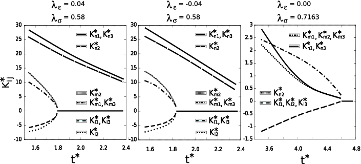
The results are presented in two Figures: 4.1 and 4.2, where the reduced elastic constants $K^{*}_{ij}={{{{\beta}}}}\,K_{ij}{{{{\rho}}}}^{-2}{{{{\epsilon}}}}^{-1}_{0}{{{{\sigma}}}}^{-6}_{0}$ are plotted against dimensionless temperature $t^{*}$ , where the units are set according to (3.20). The first one shows all the elastic constants calculated, and the second one presents a comparison of the coefficients associated with the deformation of biaxial directors for ${{{{\lambda}}}}_{{{{{\epsilon}}}}}>0$ and ${{{{\lambda}}}}_{{{{{\epsilon}}}}}<0$ .
The well known fact of equality of $K_{i1}$ and $K_{i3}$ for $i=m,n,l$ (called a splay-bend degeneracy for uniaxial director) was found to be in force for all of the directors, which follows from the lack of director dependence in low-density approximation for pair direct correlation function $c_{2}$ [121], and is due to keeping only leading order parameters in formula (2.48). It can be immediately seen from Fig. 4.1 that one of the elastic constants is always negative, this is a reflection of the impossibility of performing the distortion of only one director from the orthogonal set without affecting the other. The values of the constants corresponding to the biaxial directors are relatively low as compared with the uniaxial ones, both for opposite and same sign of the energy and shape biaxiality. Close to the uniaxial – biaxial nematic transition the biaxial constants became equal, as can be seen in Fig. 4.2. The situation changes qualitatively when we approach the Landau point. There the splay-bend degeneracy evolves to the equality of all the constants for biaxial directors ${{\mathbf{\hat{l}}}}$ and ${{\mathbf{\hat{m}}}}$ : $K_{l1}=K_{l2}=K_{l3}$ and $K_{m1}=K_{m2}=K_{m3}$ , and the latter become dominant.
Fig. 4.2 shows the biaxial constants for two cases of the biaxiality of energy: ${{{{\lambda}}}}_{{{{{\epsilon}}}}}=-0.04$ and ${{{{\lambda}}}}_{{{{{\epsilon}}}}}=0.04$ . It can be seen that although for ${{{{\lambda}}}}_{{{{{\epsilon}}}}}<0$ the constants are higher there is no new quality revealed for the case of opposite signs of ${{{{\lambda}}}}_{{{{{\sigma}}}}}$ and ${{{{\lambda}}}}_{{{{{\epsilon}}}}}$ .

4.1.2 Summary

We have calculated the set of elastic constants for the biaxial Gay-Berne model in the low-density approximation. Taken into account the importance of the elastic issues, it seemed only fair to present the above study to give some insight into the effects of elastic deformations in the biaxial nematic phase formed by the molecules interacting via the biaxial Gay-Berne potential [36].
As we can see from Fig. 4.2, the models of opposite and same sign of shape and energy biaxiality do not give significantly different elastic constants. The previous analysis of bifurcation diagrams was also unable to account for the apparent diversity of those cases, which was discovered in Monte Carlo simulations [35], its sources, therefore, must lie elsewhere; we address this issue in the next section.
It is possible that the constants associated with biaxial directors are, comparing to uniaxial ones, too small and thermal fluctuations cause the lack of biaxial nematic ordering in experiment. The above results show that in the vicinity of Landau point at $({{{{\lambda}}}}_{{{{{\sigma}}}}},{{{{\lambda}}}}_{{{{{\epsilon}}}}})=(0.7163,0.0)$ the ratios of the elastic constants significantly change. For self-dual ${{{{\lambda}}}}_{{{{{\sigma}}}}}$ , at temperature $10$ % lower than the $t^{*}$ of $Iso$ – $\textnormal{N}_{B}$ transition they are $K_{l1}:K_{m1}:K_{n1}=-0.71:2.46:1.0$ (at $t^{*}=4.14$ ) as compared to $K_{l1}:K_{m1}:K_{n1}=-0.18:0.33:1.0$ (at $t^{*}=1.65$ ; $10$ % lower than $t^{*}$ for $\textnormal{N}_{U+}$ – $\textnormal{N}_{B}$ transition) in rod-like regime for ${{{{\lambda}}}}_{{{{{\sigma}}}}}=0.58$ and ${{{{\lambda}}}}_{{{{{\epsilon}}}}}=-0.04$ . As we can see one of the biaxial constants associated with biaxial director is dominant at self-dual point. However, a more detailed study, possibly involving bent-core molecules is needed.
In the pursuit of the factors playing a role in stabilisation of the biaxial nematic, we continue to the next section, where we make some comments on the simplest smectic phases.

4.2 Orthogonal smectic phases

As we have seen, both theoretical and experimental studies predict a stable biaxial nematic for bent-core molecules. However, in those systems the phase diagrams are dominated by smectic structures. Also one possible threat for the experimental observation of the spatially uniform biaxial phase comes from the strong possibility that the spatially non-uniform liquid crystal state can gain stability instead. Therefore it is important to study the competition between smectic and nematic phases. It seems, therefore, important to include those in the analysis. This section is intended as an introduction to a more complete study since the equations presented here need to be solved and analysis of whether the smectic phases win over biaxial nematic needs to be conduced in more detail.
There is a great variety of known smectic structures, and accordingly great interest is given to the investigation of materials that exhibit this kind of behaviour. Without trying to be exhaustive, we can mention the problem of the tricritical point on the line of uniaxial nematic-smectic-A transition, existence of which is still a matter of discussion, after over 32 years of research (see e.g. [77, 122]), and a rich number of higher ordered smectics, known as $B_{n}$ phases ( $n=1,\dots,7$ ), discovered in bent-core systems (see, e.g. [67]).
In present section we briefly show the extension of the previous formalism to the case of the simplest spatially non-uniform liquid crystal states: the orthogonal uniaxial and biaxial smectics. We start with an example of the order parameters calculated in $L=2$ model including the smectic phases. Keeping in mind that the biaxial nematic phase range can be severely limited by the spatially non-uniform states, we again address the issue of opposite signs of energy and shape biaxiality (stronger molecular lateral attractions). As we mentioned, only for this model the simulations [35] discovered stable $\textnormal{N}_{B}$ . We show how the range of biaxial nematic phase depends on the relative sign of ${{{{\lambda}}}}_{{{{{\epsilon}}}}}$ and ${{{{\lambda}}}}_{{{{{\sigma}}}}}$ (defined in (3.31)). Then, as an introduction to a more complete study, we show the additional bifurcation formulas for 5 transitions involving the layered phases, these are nematic biaxial – smectic biaxial, nematic uniaxial – smectic uniaxial, nematic uniaxial – smectic biaxial, isotropic – smectic biaxial, and isotropic – smectic uniaxial. The numerical evaluation of these equations is yet to come. Firstly, we describe the basic smectic phases, and then show the usual methods used in the description of those structures.

The simplest smectic phase is the so-called smectic-A ( $Sm\textnormal{A}$ ). It is characterized by a long-range ordering of the orientational degrees of freedom, in the same way the nematic phase is; however, the positions of molecular centres of masses are not distributed randomly; there exists a tendency for them to on average align in layers perpendicular to the nematic director ${{\mathbf{\hat{n}}}}$ , while in each layer there is no long range translational order. Therefore a modulation of the density is visible. The inversion symmetry ${{\mathbf{\hat{n}}}}\rightarrow-{{\mathbf{\hat{n}}}}$ and invariance under the rotation around ${{\mathbf{\hat{n}}}}$ are upheld. Snapshot of such structure is pictured in Fig. 4.3. Since the layers are perpendicular to the director, $Sm\textnormal{A}$ belongs to the class of orthogonal smectics; and due to the rotational symmetry around ${{\mathbf{\hat{n}}}}$ this state is considered to be of uniaxial symmetry, and will be referred to by $Sm\textnormal{A}_{U}$ . It is possible that the biaxial nematic phase acquires the tendency to form orthogonal smectic layers. In that case the state becomes smectic with three directors, i.e., a biaxial smectic-A ( $Sm\textnormal{A}_{B}$ ). Interestingly, the first historically discovered biaxially ordered phase was smectic [123]. Presently, we will only consider biaxial and uniaxial $Sm\textnormal{A}$ , for a description of layered structures with higher degree of order see, e.g., [64].
In the smectic regime the one-particle distribution function cannot depend only on orientational degrees of freedom. To account for the average tendency of centres of mass to align in layers, it has to take, at least, one spatial direction as an argument. Traditionally it is denoted by ${\vec{\mathbf{z}}}$ , and because it is chosen to be parallel to the uniaxial director $\hat{{\mathbf{n}}}$ : ${\vec{\mathbf{z}}}=z{{\mathbf{\hat{n}}}}$ we can conclude that $P(\hat{\mbox{\boldmath{$\Omega$}}},\vec{\mathbf{z}})=P(\hat{\mbox{\boldmath{$\Omega$}}},z)$ . Since $P(\hat{\mbox{\boldmath{$\Omega$}}},z)$ has to be periodic: $P(\hat{\mbox{\boldmath{$\Omega$}}},z)=P(\hat{\mbox{\boldmath{$\Omega$}}},z+d)$ , where $d$ stands for layer thickness, usually close to the full length of the constituent molecules, we employ the usual expansion in the Fourier series:

P(\hat{\mbox{\boldmath{$\Omega$}}},z)=\sum_{l,p,q}\frac{2\,l+1}{8\,{{{{\pi}}}}^{2}d}\langle\Delta^{(l)}_{p,q}\rangle\Delta^{(l)}_{p,q}(\hat{\mbox{\boldmath{$\Omega$}}})+\sum_{l,p,q,n}\frac{2l+1}{4{{{{\pi}}}}^{2}d}S^{\,(l,n)}_{\,p,q}(z,\hat{\mbox{\boldmath{$\Omega$}}})\langle S^{\,(l,n)}_{\,p,q}\rangle\,,

(4.7)

where the summation as usual goes over $0\leq p,q\leq l$ , $l>0$ even, and $n>0$ , and where

\langle S^{\,(l,n)}_{\,m,k}\rangle=\int d\hat{\mbox{\boldmath{$\Omega$}}}\int^{d}_{0}dz\,P(\hat{\mbox{\boldmath{$\Omega$}}},z)S^{\,(l,n)}_{\,m,k}(\hat{\mbox{\boldmath{$\Omega$}}},z)\,.

(4.8)

and where the new base functions are defined as

S^{\,(l,n)}_{\,m,k}(\hat{\mbox{\boldmath{$\Omega$}}},z)=\Delta^{(l)}_{m,k}(\hat{\mbox{\boldmath{$\Omega$}}})cos\left(\frac{2{{{{\pi}}}}\,n\,z}{d}\right)\,.

(4.9)

They form an orthogonal set;

\int d\hat{\mbox{\boldmath{$\Omega$}}}\int^{d}_{0}dz\,S^{\,(l,n)^{\phantom{\prime}}}_{\,m,k}(\hat{\mbox{\boldmath{$\Omega$}}},z)S^{\,(l^{\prime},n^{\prime})}_{\,m^{\prime},k^{\prime}}(\hat{\mbox{\boldmath{$\Omega$}}},z)=\frac{4{{{{\pi}}}}^{2}d}{2\,l+1}{{{{\delta}}}}_{l,l^{\prime}}{{{{\delta}}}}_{m,m^{\prime}}{{{{\delta}}}}_{k,k^{\prime}}{{{{\delta}}}}_{n,n^{\prime}}\,.

(4.10)

Similarly to the previous analysis we take $\langle S^{\,(l,n)}_{\,m,k}\rangle$ with $l=0,2$ and $n=1$ as leading order parameters; non-zero value of $\langle S^{\,(0,1)}_{\,0,0}\rangle$ and $\langle S^{\,(2,1)}_{\,0,0}\rangle$ indicates the uniaxial smectic-A, while $\langle S^{\,(2,1)}_{\,2,2}\rangle$ vanishes in $Sm\textnormal{A}_{U}$ and becomes non-zero in biaxial smectic $Sm\textnormal{A}_{B}$ . In the isotropic phase all $\langle S^{\,(l,n)}_{\,m,k}\rangle=0$ for $l,n>0$ .
In the expansion of pair direct correlation function (2.44) new terms are introduced, namely

c_{2}({\hat{\mbox{\boldmath{$\Omega$}}}}^{\prime-1}\hat{\mbox{\boldmath{$\Omega$}}},z)=c_{2}({\hat{\mbox{\boldmath{$\Omega$}}}}^{\prime-1}\hat{\mbox{\boldmath{$\Omega$}}})+w_{s}S^{\,(0)}_{\,0,0}(z)+\sum_{m,n}w_{m,n}S^{\,(2,1)}_{\,m,n}({\hat{\mbox{\boldmath{$\Omega$}}}}^{\prime-1}\hat{\mbox{\boldmath{$\Omega$}}},z)\,,

(4.11)

where $w_{s}$ , $w_{m,n}$ need to be calculated numerically, using, e.g. low-density approximation (3.1)-(3.2). They are integrals of $c_{2}({\hat{\mbox{\boldmath{$\Omega$}}}}^{\prime-1}\hat{\mbox{\boldmath{$\Omega$}}},z)$ with $S^{\,(2,1)}_{\,m,n}({\hat{\mbox{\boldmath{$\Omega$}}}}^{\prime-1}\hat{\mbox{\boldmath{$\Omega$}}},z)$ , as can be easily obtained with help of orthogonality relations (4.10). Since we know that the terms with angular momentum index $l=2$ will give the leading contribution to the bifurcation, we already truncated the above expansion accordingly; the same argument works for the Fourier series index $n$ . Since the leading contribution to bifurcation comes from $n=1$ , we can fix it, and simplify the notation by using in further calculations $S^{\,(2)}_{\,m,n}({\hat{\mbox{\boldmath{$\Omega$}}}}^{\prime-1}\hat{\mbox{\boldmath{$\Omega$}}},z)\equiv S^{\,(2,1)}_{\,m,n}({\hat{\mbox{\boldmath{$\Omega$}}}}^{\prime-1}\hat{\mbox{\boldmath{$\Omega$}}},z)$ and $\langle S^{\,(2)}_{\,m,n}\rangle\equiv\langle S^{\,(2,1)}_{\,m,n}\rangle$ . Now we can derive the bifurcation equations corresponding to the additional phase transitions from isotropic, uniaxial, or biaxial nematic to uniaxial or biaxial smectics. However, before we present these, we show order parameters calculated using the self–consistent equation (2.27) with the above formulas.

4.2.1 Order parameters in $L=2$ model

In present section we show an alternative method of obtaining the phase diagram following from the solutions of the self–consistent equation (2.27) in $L=2$ model, i.e., we take into account the expansion of $c_{2}$ (4.11), calculate the coefficients $c^{(2)}_{m,n}$ , $w_{s}$ , $w_{m,n}$ by numerical methods (see Appendix 7), and work out the non-linear integral equations for order parameters. In the calculations we used low-density approximation, setting $c_{2}({\hat{\mbox{\boldmath{$\Omega$}}}}^{\prime-1}\hat{\mbox{\boldmath{$\Omega$}}},z-z^{\prime})=\exp[-{{{{\beta}}}}\,U]-1$ , where $U$ is the biaxial Gay-Berne potential (3.21). In the case of $w_{s}$ and $w_{m,n}$ the calculations were significantly longer, due to the fact that the integral over $z-z^{\prime}$ has to be calculated in the similar way as integral over $r$ in $c^{(2)}_{m,n}$ , as mentioned in Appendix 7. The equation (2.27) now becomes:

P(\hat{\mbox{\boldmath{$\Omega$}}},z)=Z^{-1}_{s}\exp\left[{{{{\rho}}}}\int d{\hat{\mbox{\boldmath{$\Omega$}}}}^{\prime}\int^{d}_{0}dz^{\prime}\,c^{(2)}_{2}({\hat{\mbox{\boldmath{$\Omega$}}}}^{\prime-1}\hat{\mbox{\boldmath{$\Omega$}}},z-z^{\prime})P({\hat{\mbox{\boldmath{$\Omega$}}}}^{\prime},z^{\prime})\right]\,,

(4.12)

where $Z_{s}=\int d\hat{\mbox{\boldmath{$\Omega$}}}\,dz\,\exp\left[{{{{\rho}}}}\int d{\hat{\mbox{\boldmath{$\Omega$}}}}^{\prime}dz^{\prime}\,c^{(2)}_{2}({\hat{\mbox{\boldmath{$\Omega$}}}}^{\prime-1}\hat{\mbox{\boldmath{$\Omega$}}},z-z^{\prime})P({\hat{\mbox{\boldmath{$\Omega$}}}}^{\prime},z^{\prime})\right]$ , and where

\begin{split}c^{(2)}_{2}({\hat{\mbox{\boldmath{$\Omega$}}}}^{\prime-1}\hat{\mbox{\boldmath{$\Omega$}}},z-z^{\prime})=&\sum_{m,n\in\{0,2\}}c^{(2)}_{m,n}\Delta^{(2)}_{m,n}({\hat{\mbox{\boldmath{$\Omega$}}}}^{\prime-1}\hat{\mbox{\boldmath{$\Omega$}}})\\ &+w_{s}S^{\,(0)}_{\,0,0}(z-z^{\prime})+\sum_{m,n\in\{0,2\}}w_{m,n}S^{\,(2)}_{\,m,n}({\hat{\mbox{\boldmath{$\Omega$}}}}^{\prime-1}\hat{\mbox{\boldmath{$\Omega$}}},z-z^{\prime})\,.\end{split}

(4.13)

In terms of order parameters the Eq. (4.12) can be written (similarly to Eq. (2.53)) as:

\begin{split}\langle S^{\,(2)}_{\,m,n}\rangle=Z^{-1}_{s}\int&d\hat{\mbox{\boldmath{$\Omega$}}}\int^{d}_{0}dz\,S^{\,(2)}_{\,m,n}(\hat{\mbox{\boldmath{$\Omega$}}},z)\\ &\exp\left[{{{{\rho}}}}\int d{\hat{\mbox{\boldmath{$\Omega$}}}}^{\prime}\int^{d}_{0}dz^{\prime}\,c^{(2)}_{2}({\hat{\mbox{\boldmath{$\Omega$}}}}^{\prime-1}\hat{\mbox{\boldmath{$\Omega$}}},z-z^{\prime})P({\hat{\mbox{\boldmath{$\Omega$}}}}^{\prime},z^{\prime})\right]\,.\end{split}

(4.14)

Solving Eqs. (4.14) and Eqs. (2.52) for $\langle\Delta^{(2)}_{m,n}\rangle$ in the iterative manner we can calculate the order parameters for given density and temperature and estimate the location of phase transitions.
An example of the results obtained in the way described above is presented in Fig. 4.4. It shows dominant order parameters for the biaxial Gay-Berne model (Sec. 3.4.2) as function of temperature for dimensionless density ${{{{\rho}}}}^{*}=0.18$ (see Eq. (3.20)). There are $9$ relevant $\langle S^{\,(2)}_{\,m,n}\rangle$ , all were calculated, but we only plot the largest ones. The range of biaxial nematic phase is limited by biaxial smectic, and, as can be seen by comparing Fig. 4.4(a) with Fig. 4.4(b), depends on the sign of energy biaxiality ${{{{\lambda}}}}_{{{{{\epsilon}}}}}$ . More precisely, the region of stable $\textnormal{N}_{B}$ is wider in case of stronger lateral interactions (where molecules are stronger attracted to their sides, i.e., side-to-side configuration gives the deepest minimum, see Fig. 3.5) for ${{{{\lambda}}}}_{{{{{\sigma}}}}}>0$ and ${{{{\lambda}}}}_{{{{{\epsilon}}}}}<0$ than for same signs of the biaxialities. In that respect the present approach can explain why Monte Carlo simulations discovered stable $\textnormal{N}_{B}$ only for opposite signs of ${{{{\lambda}}}}_{{{{{\epsilon}}}}}$ and ${{{{\lambda}}}}_{{{{{\sigma}}}}}$ [35]. Probably the spatially non-uniform structures gained stability earlier. As we can see, the transition from biaxial nematic leads directly to biaxial smectic, which is in agreement with [35], also $L=2$ model gives $\langle S^{\,(0)}_{\,0,0}\rangle=\langle S^{\,(2)}_{\,0,0}\rangle$ . The results obtained from the solution of the self–consistent equation for order parameters for $Iso$ – $\textnormal{N}_{U+}$ and $\textnormal{N}_{U+}$ – $\textnormal{N}_{B}$ transitions are equivalent to those obtained by bifurcation analysis, the main difference being the calculation time, which is significantly shorter in case of Eq. (2.47) and Eq. (2.58). Thus it is useful to have analogical equations for the bifurcations involving $Sm\textnormal{A}_{B}$ and $Sm\textnormal{A}_{U}$ . We present them in the following section.

4.2.2 Bifurcation equations

Given the above it is obvious that we have a larger number of possible bifurcation scenarios. Disregarding the smectic phase as a reference, we can expect five additional bifurcations; those are: $\textnormal{N}_{B}$ – $Sm\textnormal{A}_{B}$ , $\textnormal{N}_{U}$ – $Sm\textnormal{A}_{U}$ , $\textnormal{N}_{U}$ – $Sm\textnormal{A}_{B}$ , $Iso$ – $Sm\textnormal{A}_{U}$ , and $Iso$ – $Sm\textnormal{A}_{B}$ . We list the bifurcation equations (2.33) in the form of Eq. (2.39). They follow, as in the previous cases, from the expansion

p_{1}(\hat{\mbox{\boldmath{$\Omega$}}},z)=\sum_{l,m,n}s^{(l)}_{m,n}S^{\,(l)}_{\,m,n}(\hat{\mbox{\boldmath{$\Omega$}}},z)\,,

(4.15)

which is equivalent to Eq. (2.35). The derivation is analogical to the one presented for the spatially uniform states. We show the equations with the help of the bifurcation matrix ${\mathbf{\hat{\mbox{\boldmath{${{{{\omega}}}}$}}}}}^{(2)}$ , and as in case of Eq. (2.39) the bifurcation point ${{{{\rho}}}}_{0}$ is determined from the roots of the characteristic polynomial, Eq. (2.41), which for the present normalizations can be written as

\det\left[{\mathbf{\hat{\mbox{\boldmath{${{{{\omega}}}}$}}}}}^{(2)}-2\,{{{{\rho}}}}^{-1}_{0}{\mathbf{\hat{\mathbbm{1}}}}\right]=0\,,

(4.16)

where ${\mathbf{\hat{\mathbbm{1}}}}$ stands for the unit matrix. From the solutions of the above equation the bifurcation point is chosen as the one with the lowest ${{{{\rho}}}}_{0}$ , as was described previously in Sec. 2.2.2. In the following all the averages $\langle\Delta^{(l)}_{m,n}\rangle$ are calculated in the reference state.
1. Nematic uniaxial – smectic uniaxial.
In this case the bifurcation matrix is $3x3$ , and the bifurcation equation reads

\left(\begin{array}[]{c}s^{(0)}_{0,0}\\ s^{(2)}_{0,0}\\ s^{(2)}_{0,2}\\ \end{array}\right)=\frac{{{{{\rho}}}}_{0}}{2}{\mathbf{\hat{\mbox{\boldmath{${{{{\omega}}}}$}}}}}^{(2)}_{1}\left(\begin{array}[]{c}s^{(0)}_{0,0}\\ s^{(2)}_{0,0}\\ s^{(2)}_{0,2}\\ \end{array}\right)\,,

(4.17)

where

{\mathbf{\hat{\mbox{\boldmath{${{{{\omega}}}}$}}}}}^{(2)}_{1}\equiv\left(\begin{array}[]{ccc}w_{s}&w_{0,0}\langle\Delta^{(2)}_{0,0}\rangle+w_{0,2}\langle\Delta^{(2)}_{0,2}\rangle&w_{2,0}\langle\Delta^{(2)}_{0,0}\rangle+w_{2,2}\langle\Delta^{(2)}_{0,2}\rangle\\ w_{s}\langle\Delta^{(2)}_{0,0}\rangle&A_{0}w_{0,0}+B_{0}w_{0,2}&A_{0}w_{2,0}+B_{0}w_{2,2}\\ w_{s}\langle\Delta^{(2)}_{0,2}\rangle&B_{0}w_{0,0}+C_{0}w_{0,2}&B_{0}w_{2,0}+C_{0}w_{2,2}\end{array}\right)\,,

(4.18)

and where

\begin{split}35\,A_{0}=&\,7+10\langle\Delta^{(2)}_{0,0}\rangle+18\langle\Delta^{(4)}_{0,0}\rangle\,,\\ 35\,B_{0}=&\,-10\langle\Delta^{(2)}_{0,2}\rangle+3\sqrt{15}\langle\Delta^{(4)}_{0,2}\rangle\,,\\ 35\,C_{0}=&\,7-10\langle\Delta^{(2)}_{0,0}\rangle+3\langle\Delta^{(4)}_{0,0}\rangle+3\sqrt{35}\langle\Delta^{(4)}_{0,4}\rangle\,.\end{split}

(4.19)

2. Nematic uniaxial – smectic biaxial.
Here the uniaxial smectic parameters $s^{(0)}_{0,0}$ , $s^{(2)}_{0,0}$ , and $s^{(2)}_{0,2}$ bifurcate independently, along Eq. (4.17), and the equation for remaining coefficients is as follows:

\left(\begin{array}[]{c}s^{(2)}_{2,0}\\ s^{(2)}_{2,2}\\ \end{array}\right)=\frac{{{{{\rho}}}}_{0}}{2}{\mathbf{\hat{\mbox{\boldmath{${{{{\omega}}}}$}}}}}^{(2)}_{2}\left(\begin{array}[]{c}s^{(2)}_{2,0}\\ s^{(2)}_{2,2}\\ \end{array}\right)\,,

(4.20)

where

{\mathbf{\hat{\mbox{\boldmath{${{{{\omega}}}}$}}}}}^{(2)}_{2}=\left(\begin{array}[]{ll}A_{0}w_{0,0}+B_{0}w_{0,2}&A_{0}w_{2,0}+B_{0}w_{2,2}\\ B_{0}w_{0,0}+B_{2}w_{0,2}&B_{0}w_{2,0}+B_{2}w_{2,2}\end{array}\right)\,,

(4.21)

and where

\begin{split}35\,A_{0}=&\,7-10\langle\Delta^{(2)}_{0,0}\rangle+3\langle\Delta^{(4)}_{0,0}\rangle\,,\\ 70\,B_{0}=&\,20\langle\Delta^{(2)}_{0,2}\rangle+\sqrt{15}\langle\Delta^{(4)}_{0,2}\rangle\,,\\ 70\,B_{2}=&\,14+20\langle\Delta^{(2)}_{0,0}\rangle+\langle\Delta^{(4)}_{0,0}\rangle+\sqrt{35}\langle\Delta^{(4)}_{0,4}\rangle\,.\end{split}

(4.22)

3. Nematic biaxial – smectic biaxial.
The bifurcation eigenproblem, due to the non-trivial structure of the reference state, involves $5x5$ matrix. The equation reads

\left(\begin{array}[]{c}s^{(0)}_{0,0}\\ s^{(2)}_{0,0}\\ s^{(2)}_{0,2}\\ s^{(2)}_{2,0}\\ s^{(2)}_{2,2}\\ \end{array}\right)=\frac{{{{{\rho}}}}_{0}}{2}{\mathbf{\hat{\mbox{\boldmath{${{{{\omega}}}}$}}}}}^{(2)}_{3}\left(\begin{array}[]{c}s^{(0)}_{0,0}\\ s^{(2)}_{0,0}\\ s^{(2)}_{0,2}\\ s^{(2)}_{2,0}\\ s^{(2)}_{2,2}\\ \end{array}\right)\,,

(4.23)

where

{\mathbf{\hat{\mbox{\boldmath{${{{{\omega}}}}$}}}}}^{(2)}_{3}=\left(\begin{array}[]{ccccc}({\mathbf{\hat{\mbox{\boldmath{${{{{\omega}}}}$}}}}}^{(2)}_{1})_{0,0}&({\mathbf{\hat{\mbox{\boldmath{${{{{\omega}}}}$}}}}}^{(2)}_{1})_{0,1}&({\mathbf{\hat{\mbox{\boldmath{${{{{\omega}}}}$}}}}}^{(2)}_{1})_{0,2}&A_{0}&A_{2}\\ ({\mathbf{\hat{\mbox{\boldmath{${{{{\omega}}}}$}}}}}^{(2)}_{1})_{1,0}&({\mathbf{\hat{\mbox{\boldmath{${{{{\omega}}}}$}}}}}^{(2)}_{1})_{1,1}&({\mathbf{\hat{\mbox{\boldmath{${{{{\omega}}}}$}}}}}^{(2)}_{1})_{1,2}&Dw_{0,2}-Cw_{0,0}&Dw_{2,2}-Cw_{2,0}\\ ({\mathbf{\hat{\mbox{\boldmath{${{{{\omega}}}}$}}}}}^{(2)}_{1})_{2,0}&({\mathbf{\hat{\mbox{\boldmath{${{{{\omega}}}}$}}}}}^{(2)}_{1})_{2,1}&({\mathbf{\hat{\mbox{\boldmath{${{{{\omega}}}}$}}}}}^{(2)}_{1})_{2,2}&Dw_{0,0}+Gw_{0,2}&Dw_{2,0}+Gw_{2,2}\\ B_{0}&Dw_{0,2}-Cw_{0,0}&Dw_{2,2}-Cw_{2,0}&Iw_{0,2}-Hw_{0,0}&Iw_{2,2}-Hw_{2,0}\\ B_{2}&Dw_{0,0}+Gw_{0,2}&Dw_{2,0}+Gw_{2,2}&Iw_{0,0}+Jw_{0,2}&Iw_{2,0}+Jw_{2,2}\end{array}\right)\,,

and where

\begin{split}A_{n}=&\,\sum_{m\in\{0,2\}}w_{n,m}\langle\Delta^{(2)}_{2,m}\rangle\,,\,\,B_{n}=w_{s}\langle\Delta^{(2)}_{2,n}\rangle\,,\\ 70\,C=&\,20\langle\Delta^{(2)}_{2,0}\rangle-6\sqrt{15}\langle\Delta^{(4)}_{2,0}\rangle\,,\\ 14\,D=&\,4\langle\Delta^{(2)}_{2,2}\rangle+3\langle\Delta^{(4)}_{2,2}\rangle\,,\\ 70\,F=&\,-7+10\langle\Delta^{(2)}_{0,0}\rangle-3\langle\Delta^{(4)}_{0,0}\rangle-3\sqrt{35}\langle\Delta^{(4)}_{0,4}\rangle\,,\\ 70\,G=&\,20\langle\Delta^{(2)}_{2,0}\rangle+\sqrt{15}\langle\Delta^{(4)}_{2,0}\rangle+5\sqrt{21}\langle\Delta^{(4)}_{2,4}\rangle\,,\\ 35\,H=&\,-7+10\langle\Delta^{(2)}_{0,0}\rangle-3\langle\Delta^{(4)}_{0,0}\rangle-3\sqrt{35}\langle\Delta^{(4)}_{4,0}\rangle\,,\\ 70\,I=&\,20\langle\Delta^{(2)}_{0,2}\rangle+\sqrt{15}\langle\Delta^{(4)}_{0,2}\rangle+5\sqrt{21}\langle\Delta^{(4)}_{4,2}\rangle\,,\\ 70\,J=&\,14+20\langle\Delta^{(2)}_{0,0}\rangle+\langle\Delta^{(4)}_{0,0}\rangle+\sqrt{35}\langle\Delta^{(4)}_{0,4}\rangle+\sqrt{35}\langle\Delta^{(4)}_{4,0}\rangle+35\langle\Delta^{(4)}_{4,4}\rangle\,.\end{split}

(4.24)

4. Isotropic – biaxial smectic transition.
In this case we have the simplest bifurcation matrix, since the reference state has trivial, isotropic structure. The equation is as follows:

\left(\begin{array}[]{c}s^{(0)}_{0,0}\\ s^{(2)}_{0,0}\\ s^{(2)}_{0,2}\\ s^{(2)}_{2,0}\\ s^{(2)}_{2,2}\\ \end{array}\right)=\frac{{{{{\rho}}}}_{0}}{2}{\mathbf{\hat{\mbox{\boldmath{${{{{\omega}}}}$}}}}}^{(2)}_{4}\left(\begin{array}[]{c}s^{(0)}_{0,0}\\ s^{(2)}_{0,0}\\ s^{(2)}_{0,2}\\ s^{(2)}_{2,0}\\ s^{(2)}_{2,2}\\ \end{array}\right)\,,

(4.25)

where

{\mathbf{\hat{\mbox{\boldmath{${{{{\omega}}}}$}}}}}^{(2)}_{4}\equiv 2\left(\begin{array}[]{ccccc}w_{s}-\frac{1}{{{{{\rho}}}}_{0}}&0&0&0&0\\ 0&w_{0,0}-\frac{9}{{{{{\rho}}}}_{0}}&w_{2,0}&0&0\\ 0&w_{0,2}&w_{2,2}-\frac{9}{{{{{\rho}}}}_{0}}&0&0\\ 0&0&0&w_{0,0}-\frac{9}{{{{{\rho}}}}_{0}}&w_{2,0}\\ 0&0&0&w_{0,2}&w_{2,2}-\frac{9}{{{{{\rho}}}}_{0}}\end{array}\right)\,.

(4.26)

As we can see only the order parameters $\langle S^{\,(l,n)}_{\,q,p}\rangle$ for $l=2,4$ and $n=1$ are needed to localize the bifurcation point. In case of $\textnormal{N}_{U}$ – $Sm\textnormal{A}_{B}$ transition (2), the uniaxial and biaxial parameters bifurcate independently, and the equations involving uniaxial ones are the same as in case of $\textnormal{N}_{U}$ – $Sm\textnormal{A}_{U}$ (1). It was also the case for the bifurcations where isotropic phase was taken as the reference for spatially uniform states (Eq. (2.46)), only this time the bifurcation equations involving biaxial and uniaxial smectic are different, due to the non-trivial structure of the reference state. This decoupling is removed for $\textnormal{N}_{B}$ – $Sm\textnormal{A}_{B}$ case (3), where the bifurcation matrix (Eq. (4.23)) contains the elements of matrix for $\textnormal{N}_{U}$ – $Sm\textnormal{A}_{U}$ from Eq. (4.17), but the biaxial and uniaxial bifurcations do not occur separately, the coefficients are mixed. It follows from the fact that the $D_{2h}$ symmetry is not broken during this transition. In case of the isotropic reference phase, as for spatially uniform states, the coefficients associated with pure smectic order parameter $\langle S^{\,(0,1)}_{\,0,0}\rangle$ , with biaxial and uniaxial smectic, bifurcate independently.

4.2.3 Further studies

We have presented additional bifurcation equations for the transitions involving uniaxial and biaxial smectic-A phases. They extend the previously derived bifurcation equations and, with Eqs. (2.47), (2.58), present a way to study the stability of the biaxial nematic against simplest spatially non-uniform phases. The solution of those, most probably, gives similar diagrams, as those obtained by working out the self–consistent equation (4.12). As an example we presented the temperature dependence of order parameters obtained by iteratively solving the self–consistent equation. The phase sequence discovered with increase of the temperature was $Sm\textnormal{A}_{B}$ – $\textnormal{N}_{B}$ – $\textnormal{N}_{U}$ – $Iso$ . We have shown that the range of biaxial nematic phase is influenced by the opposite signs of shape and energy biaxiality. For stronger lateral forces (Fig. 4.4(a)) the temperature range ${{{{\delta}}}}t_{1}$ of $\textnormal{N}_{B}$ limited by $Sm\textnormal{A}_{B}$ was wider than the interval ${{{{\delta}}}}t_{2}$ for same signs of ${{{{\lambda}}}}_{{{{{\epsilon}}}}}$ and ${{{{\lambda}}}}_{{{{{\sigma}}}}}$ (Fig. 4.4(b)), which corresponds to the model where molecules are stronger attracted in the face-to-face configuration. The ratio of those ranges was found to be: ${{{{\delta}}}}t_{2}/{{{{\delta}}}}t_{1}=0.77$ . In some sense it partially explains the reasons as to why the model of strong lateral interactions gave $\textnormal{N}_{B}$ in Monte Carlo simulations [35]. This method is equivalent to bifurcation, but is numerically more demanding, and it is more worthwhile to consider using a trial one-particle distribution function analogical to (3.9), like

P_{trial}(\hat{\mbox{\boldmath{$\Omega$}}},z)=Z^{-1}_{trial}\exp\left[\sum_{m,n}{{{{\alpha}}}}_{mn}\Delta^{(2)}_{m,n}(\hat{\mbox{\boldmath{$\Omega$}}})+\sum_{m,n}{{{{\gamma}}}}_{m,n}S^{\,(2)}_{\,m,n}(\hat{\mbox{\boldmath{$\Omega$}}},z)\right]\,,

(4.27)

where $Z_{trial}$ ensures the normalization $\int d\hat{\mbox{\boldmath{$\Omega$}}}\,dz\,P_{trial}(\hat{\mbox{\boldmath{$\Omega$}}},z)=1$ , and minimize the free energy with respect to the parameters ${{{{\alpha}}}}_{m,n}$ and ${{{{\gamma}}}}_{m,n}$ . This method will give more accurate phase diagrams.
In the same way as we performed the analysis in search for factors that stabilize the biaxial nematic against $Iso$ or $\textnormal{N}_{U}$ states, the next step would be to localize the molecular parameters that reduce the stability of $Sm\textnormal{A}_{U}$ and $Sm\textnormal{A}_{B}$ with respect to $\textnormal{N}_{B}$ . In that way we can obtain a more complete picture of the region where thermotropic biaxial nematic is stable. Yet we already know it would not be enough. As we have mentioned, the bent-core systems exhibit a variety of sophisticated smectic phases, and the inclusion of those should also be considered.

Chapter 5 Summary and future studies

We have presented a Density Functional Theory (DFT) study on the stability of the thermotropic biaxial nematic ( $\textnormal{N}_{B}$ ) in comparison to isotropic liquid and uniaxial nematic phases, in three models of intermolecular pair potential. We started with brief description of the historical background and the research concerning biaxial nematic phase conduced so far. Then, we introduced the theoretical tools: the Density Functional Theory and bifurcation analysis, explored in the subsequent part of the thesis. We derived the bifurcation equations, in both the general and specific forms, for transitions involving spatially uniform states. We showed how the representations numbered by angular momentum index bifurcate, and that the contribution from pair direct correlation function to the bifurcation point comes only from the subspace of the order equal to the one of bifurcating representation.
In the following part, we mainly applied DFT using the low-density approximation for pair direct correlation function, with the exception of the first model, where mean field theory was used. We focused on the determination of the phase diagram at bifurcation point for spatially uniform states, and commented on elastic constants and smectic phases.
Firstly, we analysed a generic biaxial $L=2$ model [10] of the pair potential. It allowed to acquire the exact bifurcation diagram in mean field, which emphasised how the coupling constants impact the transition to biaxial nematic, Landau points, and tricritical regions. Being the simplest possible interaction giving rise to $\textnormal{N}_{B}$ , it can be used to locate the primary, effective factors influencing the stability of this mesophase in terms of the coupling constants.
We continued to investigate the biaxial Gay-Berne model [36]. It was characterized by six constants related to shape of molecules and interaction strengths. These were combined into two scalar quantities describing shape and energy biaxiality, which were used to parametrize the bifurcation diagrams. By varying these parameters we found the Landau(self-dual) points, which mark the regions where $\textnormal{N}_{B}$ is most stable in comparison to uniaxial nematic and isotropic liquid, and, therefore, allow to locate the microscopic parameters sets and their relative magnitudes most important for stabilisation of biaxial nematic. We illustrated how the shape and energy biaxiality and the inclusion of attractive forces change Landau point position. The results suggest that the so-called square root rule, which relates the axes of the hard, biaxial ellipsoids at self-dual point, is also significant for soft biaxial Gay-Berne interaction. Our analysis rendered the plane parametrized by shape and energy biaxialities and defined by the square root rule, as a good, but not only, candidate for the approximate locations of the Landau points. This conclusion needs to be confirmed by more detailed studies. The biaxial Gay-Berne interaction was also important because Monte Carlo study predicted for it a stable $\textnormal{N}_{B}$ , but only for one set of potential parameters, namely for the model of strong lateral attractions, where the molecules are more attracted to their sides than faces [35]. In our studies $\textnormal{N}_{B}$ appears stable quite easily, for many geometries, mainly because we neglect other, lower symmetric structures. In order to address this issue, we presented a preliminary analysis involving orthogonal spatially non-uniform phases. It indicated that the temperature range of biaxial nematic between biaxial smectic-A and uniaxial nematic is wider in the case identified in the simulations than for the model of the strongest face-to-face attractions.
Biaxial Gay-Berne model served as the example for the way the biaxiality of molecules and anisotropy of intermolecular forces influence the transition to the biaxial nematic phase. It was also used to confirm our findings on the contribution of the $L=2$ model of pair direct correlation function to transition points involving isotropic and nematic phases. In pursuit for the reasons for biaxial nematic formation in this model, we also calculated the set of bulk biaxial elastic constants in rod-like regime and at Landau point. Only in the vicinity of the self-dual point, relative values of biaxial constants changed significantly, namely the ones corresponding to the deformations of one of the biaxial directors became dominant.
A model that can be more closely related to the experimental studies where biaxial nematic was observed, was the system of bent-core (banana-like) molecules. We found that for banana with two uniaxial Gay-Berne arms the Landau point is not affected by the inclusion of attractive forces since it was found at the same opening angle ${{{{\gamma}}}}$ as for hard bent-core molecules [38]. In case of three uniaxial arms, Landau point was located for ${{{{\gamma}}}}$ close to the right angle, which is in agreement with some of recent observations [61]. Bent-core model was also the only one where we introduced dipole-dipole interactions and studied their influence on bifurcation diagram. Our findings indicate that the Landau point was not only shifted towards lower opening angles, but also, for three parts model a self-dual line was obtained for moderate strengths of the dipole. In light of this, we conclude that the dipole-dipole interactions and, therefore, the presence of electric dipoles in bent-core molecules are important factors in the stabilisation of $\textnormal{N}_{B}$ . Using the generalized Gay-Berne potential, we also took into account the model of two biaxial, soft ellipsoids as arms of the banana-like molecule. Bifurcation diagram showed a line of Landau points, indicating that the biaxiality of the arms is also important for the formation of biaxial nematic.

A first step towards further studies is to investigate in detail the self-dual plane for the biaxial Gay-Berne model and discuss its relation to the one following from the square root rule. Then, one should consider the smectic structures, not only orthogonal, taken into account in the last chapter, but also lower symmetric, spatially non-uniform phases. In other words, the next(difficult) question that should be asked is: what factors enlarge the region of stability of biaxial nematic with respect to smectics.
Concerning the approximations for the excess Helmholtz free energy, firstly one should take into consideration a more realistic reference state for the Taylor expansion, e.g., a system of hard molecules. Similar strategy was used in case of uniaxial molecules, and was proven successful in comparison with simulation results [100, 101, 124]. In those papers, a separation (inspired by previous studies [125] and the analogy between systems of hard spheres and hard ellipsoids [126]) of Gay-Berne potential into attractive and repulsive parts was performed. The steric part of the free energy was calculated exactly, while the contribution from the attractive forces was introduced in a perturbative manner. Probably, those approaches can be generalized to the case of biaxial ellipsoids, and some meaning of the attractive biaxial forces as well as a better agreement with simulations can be acquired. Also, next order terms in density in the Taylor expansion can be included, i.e., higher direct correlation functions can be taken into account. However, in this case the integrals become more challenging. One method of addressing this issue is a so-called weighted density approximation where the excess Helmholtz free energy depends on the density averaged with an appropriately chosen weighting function [127]. This approach was used for the case of hard biaxial molecules (spheroplatelets) [30, 31] and it can be extended to soft potentials.

There are great hopes associated with the thermotropic biaxial nematic phase, concerning not only the promising technological applications, but also a deeper understanding of the mechanisms of mesophase formulation. Equally great are the experimental and theoretical efforts to determine the factors that increase the chances of observing this state. Present work is a small contribution to this ongoing search.

{appendices}

Chapter 6 Calculation of $c_{1}$

Here we will show that the first direct correlation function is given by

c_{1}\left(x_{1},\left[{{{{\varrho}}}}\right]\right)={{{{\beta}}}}\left[{{{{\mu}}}}-V_{ext}\left(x_{1}\right)\right]-\ln{\left[\Lambda{{{{\varrho}}}}(x_{1})\right]}\,\textrm{.}

(6.1)

To achieve this we will calculate the first derivative of excessive free energy functional in two ways, from (2.18), and then using (2.15). Differentiating (2.18) with respect to ${{{{\varrho}}}}(x_{1})$ results in:

\frac{{{{{\delta}}}}{\cal{F}}\left[{{{{\varrho}}}}\right]}{{{{{\delta}}}}{{{{\varrho}}}}\left(x_{1}\right)}={{{{\beta}}}}^{-1}\ln\left[{\Lambda{{{{\varrho}}}}(x_{1})}\right]-c_{1}(x_{1},\left[{{{{\varrho}}}}\right])\,\textrm{.}

(6.2)

Using (2.15) we can find the following expression for the first derivative:

\frac{{{{{\delta}}}}{\cal{F}}\left[{{{{\varrho}}}}\right]}{{{{{\delta}}}}{{{{\varrho}}}}\left(x_{1}\right)}=\int dx_{2}\,\frac{{{{{\delta}}}}\mathbf{\Omega}\left[{{{{\psi}}}}\right]}{{{{{\delta}}}}{{{{\psi}}}}\left(x_{2}\right)}\frac{{{{{\delta}}}}{{{{\psi}}}}\left(x_{2}\right)}{{{{{\delta}}}}{{{{\varrho}}}}\left(x_{1}\right)}+\int dx_{2}\,\frac{{{{{\delta}}}}{{{{\psi}}}}\left(x_{2}\right)}{{{{{\delta}}}}{{{{\varrho}}}}\left(x_{1}\right)}{{{{\varrho}}}}(x_{2})+{{{{\psi}}}}\left(x_{1}\right)\,\textrm{,}

(6.3)

where

\frac{{{{{\delta}}}}\mathbf{\Omega}\left[{{{{\psi}}}}\right]}{{{{{\delta}}}}{{{{\psi}}}}\left(x_{2}\right)}=\int dx_{3}\,\left(\frac{{{{{\delta}}}}{\cal{F}}\left[{{{{\varrho}}}}\right]}{{{{{\delta}}}}{{{{\varrho}}}}\left(x_{3}\right)}-{{{{\psi}}}}\left(x_{3}\right)\right)\frac{{{{{\delta}}}}{{{{\varrho}}}}(x_{3})}{{{{{\delta}}}}{{{{\psi}}}}\left(x_{2}\right)}-{{{{\varrho}}}}(x_{2})=-{{{{\varrho}}}}(x_{2})\,,

(6.4)

and where we have used (2.16) to eliminate the term under the integral. We arrive at

\frac{{{{{\delta}}}}{\cal{F}}\left[{{{{\varrho}}}}\right]}{{{{{\delta}}}}{{{{\varrho}}}}\left(x_{1}\right)}={{{{\psi}}}}\left(x_{1}\right)\equiv{{{{\mu}}}}-V_{ext}\left(x_{1}\right)\,,

(6.5)

and from (6.2) and (6.5) we derive (6.1).

Chapter 7 Details of the calculations

Throughout the work we have employed certain technical methods, which were not described in detail, those belong in present appendix. Here we will describe the method of numerical integration developed to deal with the integrals that are present in Eq. (2.44) and in coefficients of Eq. (4.13), the methods of solving the self-consistent equations, and comment on the magnitude of numerical errors.

7.1 Integration procedure

Once the bifurcation equations are formulated, we are left with only one problem: the estimation of the $c^{(2)}_{m,n}$ coefficients in Eq. (2.44) (or $w_{s}$ , $w_{m,n}$ in Eq. (4.13)). They enter all of the equations for branching point (2.47), (2.58). In order to calculate them, we need a model for pair direct correlation function. We have chosen the low-density approximation, as described by Eqs. (3.1)-(3.2). Given the model two-point potential $V(x_{1},x_{2})$ , we can proceed to calculate the coefficients $c^{(2)}_{m,n}$ . That task has to be performed numerically.
We focus on the spatially uniform case; the calculations for smectic coefficients $w_{s}$ , $w_{m,n}$ are analogical. Each $c^{(2)}_{m,n}$ is, in fact, a six dimensional integral:

\begin{split}c^{(2)}_{m,n}=&\,\int^{2{{{{\pi}}}}}_{0}d{{{{\alpha}}}}\int^{{{{{\pi}}}}}_{0}d{{{{\beta}}}}\sin({{{{\beta}}}})\int^{2{{{{\pi}}}}}_{0}d{{{{\gamma}}}}\int^{2{{{{\pi}}}}}_{0}d{{{{\theta}}}}\int^{{{{{\pi}}}}}_{0}d{{{{\phi}}}}\int^{R}_{0}dr^{*}\,{r^{*}}^{2}\\ &\;\;\;\;\;\;\;\;c({{{{\alpha}}}},{{{{\beta}}}},{{{{\gamma}}}},{{{{\theta}}}},{{{{\phi}}}},r^{*})\Delta^{(2)}_{m,n}({{{{\alpha}}}},{{{{\beta}}}},{{{{\gamma}}}})\,,\\ c({{{{\alpha}}}},{{{{\beta}}}},{{{{\gamma}}}},{{{{\theta}}}},{{{{\phi}}}},r^{*})=&\,\exp\left[-V^{*}({{{{\alpha}}}},{{{{\beta}}}},{{{{\gamma}}}},{{{{\theta}}}},{{{{\phi}}}},r^{*})/t^{*}\right]-1\,,\end{split}

(7.1)

in the above ${{{{\epsilon}}}}_{0}$ sets the energy unit, as in (3.20); $V^{*}=V/{{{{\epsilon}}}}_{0}$ and stands for the two-point interaction, either biaxial Gay-Berne (Sec. 3.4) or model bent-core potential (Sec. 3.5), $t^{*}$ is a dimensionless temperature defined in (3.20). In (7.1) $R$ is a fixed maximal radius, above which the contribution to the integral is negligibly small. In case of Gay-Berne interaction the choice of $R$ is fairly obvious, since there exists a distance at which most certainly the interaction is practically zero, and the above integral numerically vanishes (it follows from the fact that Gay-Berne potential operates on relatively short distances, and the long-range, attractive tail can be at some distance considered to be negligible). However in case of dipole-dipole interaction the choice of $R$ is not that obvious, since the interaction is long range. In that case we have performed the integration (7.1) for $r^{*}\leq R_{GB}$ , where $R_{GB}$ stands for the radius where Gay-Berne interaction can be neglected, and for $r^{*}>R_{GB}$ we have integrated the expanded Meyer function. So the integrand

c({{{{\alpha}}}},{{{{\beta}}}},{{{{\gamma}}}},{{{{\theta}}}},{{{{\phi}}}},r^{*})=\left\{\begin{array}[]{lr}\exp\left[-V_{GB}/t^{*}-V_{DD}/t^{*}\right]-1,&\textnormal{for }r^{*}\leq R_{GB}\,,\\ \frac{1}{2}V^{2}_{DD}/{t^{*}}^{2},&\textnormal{for }r^{*}>R_{GB}\,.\end{array}\right.\,,

(7.2)

where $V_{GB}$ stands for Gay-Berne potential and $V_{DD}$ for dipole-dipole interaction. Later the results were verified by integrating the Meyer function symmetrized with respect to the direction of the dipole, where the symmetrization was imposed by the form of one-particle distribution function. We should keep in mind that in present approach $c({{{{\alpha}}}},{{{{\beta}}}},{{{{\gamma}}}},{{{{\theta}}}},{{{{\phi}}}},r^{*})$ contributes via the Eq. (3.2):

\frac{1}{t^{*}}{\cal{F}}_{ex}\left[P\right]/\langle N\rangle=-\frac{1}{2}{{{{\rho}}}}^{*}\int d{\hat{\mbox{\boldmath{$\Omega$}}}}^{\prime}d\hat{\mbox{\boldmath{$\Omega$}}}d^{3}\vec{\mathbf{r}}^{*}\,P({\hat{\mbox{\boldmath{$\Omega$}}}}^{\prime})c({\hat{\mbox{\boldmath{$\Omega$}}}}^{\prime-1}\hat{\mbox{\boldmath{$\Omega$}}},\vec{\mathbf{r}})P(\hat{\mbox{\boldmath{$\Omega$}}})\,.

(7.3)

This equation has physical meaning, since the equilibrium state is found as the minimum of ${\cal{F}}\left[P\right]={\cal{F}}_{id}\left[P\right]+{\cal{F}}_{ex}\left[P\right]$ . As we can see, the contribution to the above comes from symmetrized $c({\hat{\mbox{\boldmath{$\Omega$}}}}^{\prime-1}\hat{\mbox{\boldmath{$\Omega$}}},\vec{\mathbf{r}})$ . The form of Eq. (7.3) is the base of all the above assumptions used in the calculation of $c^{(2)}_{m,n}$ .

In (7.1) the integrand is a strongly oscillating function, and the straight forward approach based on the classic numerical methods is going to fail to give a precise result. All of the model pair-potentials $V(x_{1},x_{2})$ , studied here, as functions of $r^{*}$ behave as presented in Fig. 3.1(a), which means that $c({\hat{\mbox{\boldmath{$\Omega$}}}}^{\prime-1}\hat{\mbox{\boldmath{$\Omega$}}},\vec{\mathbf{r}}^{*})$ for fixed orientations depends on $r^{*}$ as in Fig. 3.1(c). We can see that the integral over the radius connecting centres of mass of the molecules pose the main problems. Therefore we have developed a ”hybrid” integration method, where the $5$ dimensional integral over orientations ${{{{\alpha}}}}$ , ${{{{\beta}}}}$ , ${{{{\gamma}}}}$ , ${{{{\theta}}}}$ , and ${{{{\phi}}}}$ was calculated using Monte Carlo (MC) method, and in each MC cycle, for fixed orientational variables, a precise adaptive¹¹ 1 This method automatically located the areas with the largest relative error, and by subsequent divisions of the interval in these regions and integration reduced it to the given level. $10$ -point Gauss quadrature method was employed. The number of Monte Carlo steps and the maximum number of subdivisions of the integration interval in $r^{*}$ were tuned up so the relative error was kept to be less than $0.5$ %. It was estimated by calculating the integral for doubled number of Monte Carlo steps and interval divisions, and comparing with less precise result. That required a maximal number of Monte Carlo steps to be $4194304$ , and on average 16 subdivisions. In Fig. 7.1 an example result of the integration is presented. We show the $c^{(2)}_{0,0}$ coefficient calculated for the biaxial Gay-Berne model for biaxial, rod-like molecule as function of the dimensionless temperature $t^{*}$ . Please recall that in order to solve the self-consistent bifurcation equations, we need to know the values of $c^{(2)}_{m,n}$ for given $t^{*}$ .
In the case of smectic phases, the integral over $z$ in coefficients $w_{s}$ , $w_{m,n}$ has to be calculated precisely. For this reason the calculations for spatially non-uniform structures were one order of magnitude longer, for the integration over $z$ was performed in the same way as over $r^{*}$ in spatially uniform case, i.e., we are left with a two dimensional integral for each Monte Carlo cycle.

7.2 Self-consistent equations

Having calculated the coefficients $c^{(2)}_{m,n}$ for given pair potential parameters, and knowing their dependence on dimensionless temperature, we could proceed to solve the bifurcation equations. In the case of transitions from isotropic phase, the equations (2.47) are ”analytical”, in the sense that once we know $c^{(2)}_{m,n}$ , we can immediately find bifurcation density for given temperature, although not explicitly, since $c^{(2)}_{m,n}$ do not have an analytic dependence on $t^{*}$ . In $\textnormal{N}_{U}$ – $\textnormal{N}_{B}$ case the Eq. (2.58) are self-consistent equations for density depending on the order parameters in the reference state, which have to be calculated also in the self-consistent manner using (3.8). In order to perform the calculations concerning the stabilisation of the reference state, and the solution of bifurcation equations (2.47),(2.58) we have constructed a Mathematica notebook.

The integration procedure was implemented in C language, compiled using The Portland Group Inc. compiler. The total CPU time consumed for the calculations, results of which are presented here, including the preliminary studies on smectic phases was $90000$ hours. The numerical analysis was performed at ICM under grant G27-8, using a cluster of 110 nodes of total 292 CPUs, of which 98 machines were IBM eServer 325 (each with two AMD Opteron 246 CPUs), and 12 were Sun v40z (each with eight AMD Opteron 875 CPUs). The work was financed by grant from MNiSW no N202 169 31/3455.

Chapter 8 Symmetry adapted functions

In current appendix we would like to present a possible derivation of orthogonal base in the space of real functions, which are defined on the orientation space, i.e., are mapping unit sphere into $\mathbb{R}$ . It is also a base in the space of solutions of bifurcation equations.
In actual calculations we have used two representations of $\Delta^{(l)}_{m,n}$ functions, one with help of Euler angles and the other with directional cosines. Also some properties of Wigner matrices were used. We will briefly write down the formulas here. We follow the notation and representation of Rose [73].

8.1 Wigner matrices

Wigner matrices $D^{(l)}_{m,n}$ are representations of the rotation operator in the spherical base in the same way the rotation matrix is in Cartesian coordinates. In present work we follow the convention used by M. E. Rose [73]. This section is devoted to the brief summary of formulas which were used to obtain the symmetry adapted version of Wigner matrices, presented in the next section.
If we consider a state ${{{{\psi}}}}_{\,l,m}$ diagonalizing the square of angular momentum and one of its components along a given axis ${{\mathbf{\hat{z}}}}$ , we can wonder how this state transforms under the rotation ${\mathbf{\hat{R}}}$ about fixed direction ${{\mathbf{\hat{n}}}}$ . From definition that transformation is described by Wigner matrices:

{{\mathbf{\hat{R}}}}{{{{\psi}}}}_{\,l,m}=\sum_{m^{{}^{\prime}}}D^{(l)}_{m^{{}^{\prime}},m}({{{{\alpha}}}},{{{{\beta}}}},{{{{\gamma}}}}){{{{\psi}}}}_{\,l,m}\,,

(8.1)

where

D^{(l)}_{m^{{}^{\prime}},m}({{{{\alpha}}}},{{{{\beta}}}},{{{{\gamma}}}})=\langle l\,m^{{}^{\prime}}\left|e^{-i{{{{\alpha}}}}{\mathbf{\hat{L}}}_{z}}e^{-i{{{{\beta}}}}{\mathbf{\hat{L}}}_{y}}e^{-i{{{{\gamma}}}}{\mathbf{\hat{L}}}_{z}}\right|l\,m\rangle\,,

(8.2)

and ${\mathbf{\hat{L}}}_{x}$ , ${\mathbf{\hat{L}}}_{y}$ , ${\mathbf{\hat{L}}}_{z}$ are the angular momentum operators.
In present study we will often encounter the relative orientation of the molecules, which means that we will need a formula for the Wigner matrices in that case. From definition we have

\begin{split}D^{(l)}_{m^{\prime},m}({\hat{\mbox{\boldmath{$\Omega$}}}}^{\prime-1}\hat{\mbox{\boldmath{$\Omega$}}})=\langle l\,m^{\prime}|{{\mathbf{\hat{R}}}}^{\prime\,-1}{{\mathbf{\hat{R}}}}|l\,m\rangle=&\,\sum_{n}\langle l\,m^{\prime}|{{\mathbf{\hat{R}}}}^{\prime\,-1}|l\,n\rangle\langle l\,n\left|{{\mathbf{\hat{R}}}}\right|l\,m\rangle=\\ &\,\sum_{n}D^{(l)\,*}_{n,m^{\prime}}({\hat{\mbox{\boldmath{$\Omega$}}}}^{\prime})D^{(l)}_{n,m^{\phantom{\prime}}}(\hat{\mbox{\boldmath{$\Omega$}}})\,,\end{split}

(8.3)

where $D^{(l)\,*}_{m,n}$ stands for complex conjugate of $D^{(l)}_{m,n}$ .
Another important property of $D^{(l)}_{m,n}$ functions are the orthogonality relations:

\int d\hat{\mbox{\boldmath{$\Omega$}}}\,D^{(l)^{\phantom{\prime}}*}_{m,n^{\phantom{\prime}}}(\hat{\mbox{\boldmath{$\Omega$}}})D^{(l^{\prime})}_{m^{\prime},n^{\prime}}(\hat{\mbox{\boldmath{$\Omega$}}})=\frac{8{{{{\pi}}}}^{2}}{2l+1}{{{{\delta}}}}_{l,l^{\prime}}{{{{\delta}}}}_{m,m^{\prime}}{{{{\delta}}}}_{n,n^{\prime}}\,.

(8.4)

We will also need a rule for integrating three Wigner matrices, we can acquire it with help of the so-called Clebsch-Gordan series (see, e.g, [73] p.57):

D^{(l_{1})}_{{{{{\mu}}}}_{1},m_{1}}D^{(l_{2})}_{{{{{\mu}}}}_{2},m_{2}}=\sum_{l}C(l_{1},l_{2},l;{{{{\mu}}}}_{1},{{{{\mu}}}}_{2})C(l_{1},l_{2},l;m_{1},m_{2})D^{(l)}_{{{{{\mu}}}}_{1}+{{{{\mu}}}}_{2},m_{1}+m_{2}}\,,

(8.5)

where $C(l_{1},l_{2},l;m_{1},m_{2})$ are Clebsch-Gordan coefficients [73], and the summation goes over the $l$ satisfying the triangle rule with $l_{1}$ and $l_{2}$ . Now using (8.4) we can obtain the following:

\begin{split}\int d\hat{\mbox{\boldmath{$\Omega$}}}\,D^{(l_{3})\,*}_{{{{{\nu}}}},n}(\hat{\mbox{\boldmath{$\Omega$}}})D^{(l_{1})}_{{{{{\mu}}}}_{1},m_{1}}(\hat{\mbox{\boldmath{$\Omega$}}})D^{(l_{2})}_{{{{{\mu}}}}_{2},m_{2}}(\hat{\mbox{\boldmath{$\Omega$}}})=&\frac{8{{{{\pi}}}}^{2}}{2l_{3}+1}C(l_{1},l_{2},l_{3};{{{{\mu}}}}_{1},{{{{\mu}}}}_{2})C(l_{1},l_{2},l_{3};m_{1},m_{2})\\ &{{{{\delta}}}}_{{{{{\mu}}}}_{1}+{{{{\mu}}}}_{2},{{{{\nu}}}}}{{{{\delta}}}}_{m_{1}+m_{2},n}\,.\end{split}

(8.6)

8.2 Derivation of $\Delta^{(l)}_{m,n}$ functions

One-particle distribution function and correlation functions, in spatially uniform case, are defined on the orientation space. Current section is devoted to the introduction of the base in the space of orientation dependent, real functions, for a given model symmetry of molecules and phase.
Lets consider a set of irreducible tensors ${\bf{T}}^{\,l}_{m}$ in spherical base. Given some symmetry group ${\cal{G}}$ , any element of the set ${\bf{T}}^{\,l}_{m}$ can be symmetrized. Namely the ${\cal{G}}$ –symmetrized form of ${\bf{T}}^{\,l}_{m}$ can be written as

\left.\widetilde{{\bf{T}}}^{\,l}_{\,m}\right|_{{\cal{G}}}\equiv N^{l}_{m}\,\frac{1}{\left|{\cal{G}}\right|}\sum_{g\in{\cal{G}}}{\cal{D}}\left(g\right){\bf{T}}^{\,l}_{m}\,,

(8.7)

where ${\cal{D}}\left(g\right)$ is the operation of symmetry element $g$ , $\left|{\cal{G}}\right|$ is the number of elements in ${\cal{G}}$ , and coefficients $N^{l}_{m}$ ensure the normalization with respect to the following scalar product:

\left.\widetilde{{\bf{T}}}^{\,l}_{\,m}\right|_{{\cal{G}}}\cdot\left.\widetilde{{\bf{T}}}^{\,l^{{}^{\prime}}}_{\,m^{{}^{\prime}}}\right|_{{\cal{G}}}=\sum_{i,j,\dots}\left[\left.\widetilde{{\bf{T}}}^{\,l}_{\,m}\right|_{{\cal{G}}}\right]_{i,j,\dots}\,\left[\left.\widetilde{{\bf{T}}}^{\,l^{{}^{\prime}}}_{\,m^{{}^{\prime}}}\right|_{{\cal{G}}}\right]_{i,j,\dots}={{{{\delta}}}}_{l,l^{{}^{\prime}}}\,{{{{\delta}}}}_{m,m^{{}^{\prime}}}\,,

(8.8)

where the summation goes over Cartesian indices. ${\bf{T}}^{\,l}_{m}$ can be built using the following relation:

{\bf{T}}^{\,l}_{m}=\sum_{m1\,m2}\left(\left.\begin{array}[]{cc}l-1&1\\ m_{1}&m_{2}\end{array}\right|\begin{array}[]{c}l\\ m\end{array}\right){\bf{T}}^{\,l-1}_{m_{1}}\otimes{\bf{T}}^{1}_{m_{2}}\,,

(8.9)

where ${\bf{T}}^{\,1}_{0}$ and ${\bf{T}}^{\,1}_{{{{{\,\pm\,}}}}1}$ are as follows:

\begin{split}{\bf{T}}^{\,1}_{0}&={\bf{z}}\,,\\ {\bf{T}}^{\,1}_{{{{{\,\pm\,}}}}1}&=\frac{{{{{\,\pm\,}}}}1}{\sqrt{2}}\left({\bf{x}}{{{{\,\pm\,}}}}i\,{\bf{y}}\right)\,.\end{split}

(8.10)

One of the issues that we are dealing with is establishing the relation between microscopic structure and macroscopic properties of the system. Usually we are given some shape of molecules with some model interaction, and we are left with a problem of determining the phase sequence. We can define the shape as invariance under some symmetry group ${\cal{G}}_{B}$ , and introduce a symmetry of the phase ${\cal{G}}_{L}$ . Then, we can build the sets of ${\cal{G}}_{B}$ and ${\cal{G}}_{L}$ – symmetrized irreducible tensors [128], and choose the base functions as following combinations: ${\bf{L}}_{n}\cdot{\bf{B}}_{m}$ where ${\bf{L}}_{n}\equiv\left.\widetilde{{\bf{T}}}^{\,l^{*}}_{\,n}\right|_{{\cal{G}}_{L}}$ and ${\bf{B}}_{m}\equiv\left.\widetilde{{\bf{T}}}^{\,l^{*}}_{\,n}\right|_{{\cal{G}}_{B}}$ (the angular momentum index $l^{*}$ is fixed¹¹ 1 We refer to the ”lowest, weakest or minimal coupling model” by $L=2$ having in mind $l^{*}=2$ from the formula above.). If we assume that both ${\cal{G}}_{m}$ and ${\cal{G}}_{l}$ are equal to $D_{2h}$ , then the only non–vanishing, real, independent, non–trivial tensors remaining after symmetrization (performed along (8.7)) are:

\begin{split}\left.\widetilde{{\bf{T}}}^{\,2}_{\,0}\right|_{D_{2h}}=&\frac{1}{\sqrt{6}}\,\left(3\,{\bf{z}}\otimes{\bf{z}}-{\bf{1}}\right)\,,\\ \left.\widetilde{{\bf{T}}}^{\,2}_{\,2}\right|_{D_{2h}}=&\frac{1}{\sqrt{2}}\,\left({\bf{x}}\otimes{\bf{x}}-{\bf{y}}\otimes{\bf{y}}\right)\,.\end{split}

(8.11)

We arrive at the set of $D_{2h}$ –symmetry adapted functions:

\begin{split}\Delta^{(2)}_{0,0}(\hat{\mbox{\boldmath{$\Omega$}}})={\bf{L}}_{0}\cdot{\bf{B}}_{0}=&\,\frac{1}{4}+\frac{3}{4}\,cos\left(2\,{{{{\beta}}}}\right)\,,\\ \Delta^{(2)}_{0,2}(\hat{\mbox{\boldmath{$\Omega$}}})={\bf{L}}_{0}\cdot{\bf{B}}_{2}=&\,\frac{\sqrt{3}}{2}cos\left(2\,{{{{\gamma}}}}\right)sin\left({{{{\beta}}}}\right)^{2}\,,\\ \Delta^{(2)}_{2,0}(\hat{\mbox{\boldmath{$\Omega$}}})={\bf{L}}_{2}\cdot{\bf{B}}_{0}=&\,\frac{\sqrt{3}}{2}cos\left(2\,{{{{\alpha}}}}\right)sin\left({{{{\beta}}}}\right)^{2}\,,\\ \Delta^{(2)}_{2,2}(\hat{\mbox{\boldmath{$\Omega$}}})={\bf{L}}_{2}\cdot{\bf{B}}_{2}=&\,\frac{1}{4}\left[3+cos\left(2\,{{{{\beta}}}}\right)\right]\,cos\left(2\,{{{{\alpha}}}}\right)\,cos\left(2\,{{{{\gamma}}}}\right)\\ &-cos\left({{{{\beta}}}}\right)sin\left(2\,{{{{\alpha}}}}\right)sin\left(2\,{{{{\gamma}}}}\right)\,,\end{split}

(8.12)

where:

\begin{split}{\bf{L}}_{0}\cdot{\bf{B}}_{0}&\equiv-\frac{1}{2}+\frac{3}{2}\left({{{\mathbf{\hat{b}}}}}_{3}\cdot{{{\mathbf{\hat{l}}}}}_{3}\right)^{2}\,,\\ {\bf{L}}_{0}\cdot{\bf{B}}_{2}&\equiv\frac{\sqrt{3}}{2}\left\{\left({{{\mathbf{\hat{b}}}}}_{1}\cdot{{{\mathbf{\hat{l}}}}}_{3}\right)^{2}-\left({{{\mathbf{\hat{b}}}}}_{2}\cdot{{{\mathbf{\hat{l}}}}}_{3}\right)^{2}\right\}\,,\\ {\bf{L}}_{2}\cdot{\bf{B}}_{0}&\equiv\frac{\sqrt{3}}{2}\left\{\left({{{\mathbf{\hat{b}}}}}_{3}\cdot{{{\mathbf{\hat{l}}}}}_{1}\right)^{2}-\left({{{\mathbf{\hat{b}}}}}_{3}\cdot{{{\mathbf{\hat{l}}}}}_{2}\right)^{2}\right\}\,,\\ {\bf{L}}_{2}\cdot{\bf{B}}_{2}&\equiv\left({{{\mathbf{\hat{b}}}}}_{1}\cdot{{{\mathbf{\hat{l}}}}}_{1}\right)^{2}+\left({{{\mathbf{\hat{b}}}}}_{2}\cdot{{{\mathbf{\hat{l}}}}}_{2}\right)^{2}-\frac{1}{2}\left({{{\mathbf{\hat{b}}}}}_{3}\cdot{{{\mathbf{\hat{l}}}}}_{3}\right)^{2}-\frac{1}{2}\,,\end{split}

(8.13)

and where ${{{{\alpha}}}},{{{{\beta}}}},{{{{\gamma}}}}$ are the Euler angles [73, 72] parametrizing the rotation transforming the laboratory frame $\left\{{{{\mathbf{\hat{l}}}}}_{1},{{{\mathbf{\hat{l}}}}}_{2},{{{\mathbf{\hat{l}}}}}_{3}\right\}$ to the body frame $\left\{{{{\mathbf{\hat{b}}}}}_{1},{{{\mathbf{\hat{b}}}}}_{2},{{{\mathbf{\hat{b}}}}}_{3}\right\}$ . The set of symmetry adapted base functions (8.12) is well known [28], in present approach we can clearly see that it is valid for $D_{2h}$ – symmetric phase and molecules. Choosing the lowest possible $l^{*}$ and neglecting higher order terms constitutes the so-called weakest coupling model. The above allows for higher $l^{*}$ to be taken into account as well as other symmetries. We see that the first of the lower indices of $\Delta^{(l)}_{m,n}(\hat{\mbox{\boldmath{$\Omega$}}})$ is associated with the symmetry of phase, while the other corresponds to the molecular symmetry group.
Next, we will present some properties of $\Delta^{(l)}_{m,n}$ functions that are useful in calculations. One of them are orthogonality relations. Those are obvious when we realize that the set (8.12) can be represented by Wigner matrices [73, 79] as was done in [28]:

\Delta^{(l)}_{m,n}(\hat{\mbox{\boldmath{$\Omega$}}})=N^{m,n}_{\Delta}\,\sum_{{{{{\sigma}}}},{{{{\sigma}}}}^{{}^{\prime}}\in\left\{-1,1\right\}}D^{(l)}_{{{{{\sigma}}}}\,m,{{{{\sigma}}}}^{{}^{\prime}}\,n}(\hat{\mbox{\boldmath{$\Omega$}}})\,,

(8.14)

where coefficient $N^{m,n}_{\Delta}$ ensures the normalization. In case of $D_{2h}$ symmetry $l$ , $m$ , and $n$ are even and positive, and

N^{a,b}_{\Delta}\equiv\left(\frac{\sqrt{2}}{2}\right)^{2+{{{{\delta}}}}_{a,0}+{{{{\delta}}}}_{b,0}}\,.

(8.15)

Above representation is useful, since the orthogonality relations for $D^{(l)}_{m,n}$ (8.4) are well known [79, 73], and we can easily see that:

\int\,d\hat{\mbox{\boldmath{$\Omega$}}}\,\Delta^{(l)^{\phantom{\prime}}}_{m,n^{\phantom{\prime}}}(\hat{\mbox{\boldmath{$\Omega$}}})\,\Delta^{(l^{\prime})}_{m^{\prime},n^{\prime}}(\hat{\mbox{\boldmath{$\Omega$}}})=N^{\,l}_{\Delta\Delta}\,{{{{\delta}}}}_{l,l^{\prime}}\,{{{{\delta}}}}_{m,m^{\prime}}\,{{{{\delta}}}}_{n,n^{\prime}}\,,\,\,N^{\,l}_{\Delta\Delta}\equiv\frac{8\,{{{{\pi}}}}^{2}}{2\,l+1}\,,

(8.16)

where ${{{{\delta}}}}_{i,j}$ stands for the Kronecker delta.
We should remember that the relation (8.14), alas in present work defined only for positive and even $l,m,n$ , can be easily extended to other molecular symmetry groups. Following the above analysis it is possible to symmetrize the spherical tensors to include symmetries lower than $D_{2h}$ , which for $l^{*}=2$ will mean the inclusion of other that even and/or positive indices $m,n$ in $\Delta^{(l)}_{m,n}$ . In that sense the analysis conduced using the symmetry adapted functions, provided they form an orthogonal base in space of real functions, can be considered general.
The pair direct correlation function depends on relative orientation, and will be expanded in the above base, therefore it is of interest to take a look at $\Delta^{(l)}_{m,n}({\hat{\mbox{\boldmath{$\Omega$}}}}^{\prime-1}\hat{\mbox{\boldmath{$\Omega$}}})$ . From the definition (8.14), and using (8.3) we have

\Delta^{(l)}_{m,n}({\hat{\mbox{\boldmath{$\Omega$}}}}^{\prime-1}\hat{\mbox{\boldmath{$\Omega$}}})=N^{m,n}_{\Delta}\,\sum_{{{{{\sigma}}}},{{{{\sigma}}}}^{\prime}\in\left\{-1,1\right\}}\left[\sum_{k}\left(-1\right)^{k-{{{{\sigma}}}}\,m}D^{(l)}_{-k,{{{{\sigma}}}}^{\phantom{\prime}}m}({\hat{\mbox{\boldmath{$\Omega$}}}}^{\prime})D^{(l)}_{k,{{{{\sigma}}}}^{\prime}\,n}(\hat{\mbox{\boldmath{$\Omega$}}})\right]\,.

(8.17)

Using the above, and orthogonality of Wigner matrices, we can write down the following integration rule:

\int\,d{\hat{\mbox{\boldmath{$\Omega$}}}}^{\prime}\,\Delta^{(l)^{\phantom{\prime}}}_{m,n^{\phantom{\prime}}}({\hat{\mbox{\boldmath{$\Omega$}}}}^{\prime-1}\hat{\mbox{\boldmath{$\Omega$}}})\,\Delta^{(l^{\prime})}_{m^{\prime},n^{\prime}}({\hat{\mbox{\boldmath{$\Omega$}}}}^{\prime})=N^{\,l}_{\Delta\Delta}N^{m,n^{\prime}}_{\Delta}\,\Delta^{(l)}_{m^{\prime},n}(\hat{\mbox{\boldmath{$\Omega$}}})\sum_{{{{{\sigma}}}},{{{{\sigma}}}}^{\prime}\in\left\{-1,1\right\}}{{{{\delta}}}}_{{{{{\sigma}}}}m,{{{{\sigma}}}}^{\prime}n^{\prime}}\,{{{{\delta}}}}_{l,l^{\prime}}\,.

(8.18)

In subsequent chapters we will also need a rule for integrating three symmetry adapted base functions which follows from relation (8.6):

\begin{split}\int\,d\hat{\mbox{\boldmath{$\Omega$}}}\,\Delta^{(l)}_{m_{1},n_{1}}(\hat{\mbox{\boldmath{$\Omega$}}})\Delta^{(2)}_{m_{2},n_{2}}(\hat{\mbox{\boldmath{$\Omega$}}})\Delta^{(2)}_{m_{3},n_{3}}(\hat{\mbox{\boldmath{$\Omega$}}})=&\frac{8\,{{{{\pi}}}}^{2}}{2\,l+1}N^{m_{1},n_{1}}_{\Delta}N^{m_{2},n_{2}}_{\Delta}N^{m_{3},n_{3}}_{\Delta}\\ &\sum_{{{{{\sigma}}}}_{i}}N^{l}_{\begin{subarray}{c}m_{1},m_{2},m_{3}\\ n_{1},n_{2},n_{3}\end{subarray}}(\left\{{{{{\sigma}}}}_{i}\right\})\,,\,\,l\in\left\{2,4\right\}\,,\end{split}

(8.19)

where we have denoted

\begin{split}N^{l}_{\begin{subarray}{c}m_{1},m_{2},m_{3}\\ n_{1},n_{2},n_{3}\end{subarray}}(\left\{{{{{\sigma}}}}_{i}\right\})\equiv&\left(-1\right)^{{{{{\sigma}}}}_{1}\,m_{1}+{{{{\sigma}}}}_{2}\,n_{1}}\\ &{{{{\delta}}}}_{{{{{\sigma}}}}_{3}\,m_{2}+{{{{\sigma}}}}_{5}\,m_{3},-{{{{\sigma}}}}_{1}\,m_{1}}{{{{\delta}}}}_{{{{{\sigma}}}}_{4}\,n_{2}+{{{{\sigma}}}}_{6}\,n_{3},-{{{{\sigma}}}}_{2}\,n_{1}}\\ &C\left(2,2,l;{{{{\sigma}}}}_{3}\,m_{2},{{{{\sigma}}}}_{5}\,m_{3}\right)C\left(2,2,l;{{{{\sigma}}}}_{4}\,n_{2},{{{{\sigma}}}}_{6}\,n_{3}\right)\,,\\ &i\in\left\{1,2,3,4,5,6\right\}\,,\end{split}

(8.20)

and where $C\left(l_{1},l_{2},l;m_{1},m_{2}\right)$ are Clebsch-Gordan coefficients [73] in decomposition of state $l,m$ on to $l_{1},m_{1}$ and $l_{2},m_{2}$ , and the summation goes over all the ${{{{\sigma}}}}$ s, each taking values of $1$ and $-1$ .

There are many ways of introducing the base functions. Most of them take into account the analysis of the symmetries involved in the problem. We have presented one possible derivation which stresses out the way in which phase and molecular symmetry come into the picture. The other way would be to postulate (8.14) by requiring the proper behaviour under the $D_{2h}$ symmetry and realness, as was done for instance in [28].

Main benefits from using the irreducible representations in present work come from clear transformation laws under rotations, built-in orthogonality, and completeness. The Cartesian tensors usually come in reducible form, and therefore present a more difficult objects when it comes to actual calcualtions. On the other hand, since we are more used to the Cartesian form, some interpretation and meaning can be retrieved more easily in that base.

Chapter 9 One-particle distribution function and order parameters

During phase transition a symmetry change takes place. In isotropic – uniaxial nematic case the rotational invariance of the disordered liquid is broken, and replaced by the symmetry under the action of elements of group containing the rotation around the director and the reflection in the perpendicular plane. One possible method to model that type of behaviour is to define some quantities that in higher symmetric phase vanish, while in more ordered structure obtain a non–zero value. Those are usually defined as averages over an ensemble of the base functions (8.12), and are called order parameters.
Of course the symmetry change happening over a phase transition has to influence the one-particle distribution function. If we employ the order parameter approach it seems natural that the distribution should be parametrized by those objects. We will begin with an example of such approach.
Lets take into account two orthogonal tripods, one associated with laboratory, usually chosen to coincide with the director frame: $\left\{{{{\mathbf{\hat{l}}}}}_{1},{{{\mathbf{\hat{l}}}}}_{2},{{{\mathbf{\hat{l}}}}}_{3}\right\}$ , and the other with the molecule: $\left\{{{{\mathbf{\hat{b}}}}}_{1},{{{\mathbf{\hat{b}}}}}_{2},{{{\mathbf{\hat{b}}}}}_{3}\right\}$ . For the moment we take into account the uniaxial nematic phase, and molecules having the symmetry of ellipsoids of revolution, and write the one-particle distribution function as:

P(\left\{{{{\mathbf{\hat{l}}}}}_{i},{{{\mathbf{\hat{b}}}}}_{i}\right\})={{{{\delta}}}}\,\left({{{\mathbf{\hat{b}}}}}_{1}\cdot{{{\mathbf{\hat{l}}}}}_{3}\right)^{2}+{{{{\eta}}}}\,\left({{{\mathbf{\hat{b}}}}}_{2}\cdot{{{\mathbf{\hat{l}}}}}_{3}\right)^{2}+{{{{\vartheta}}}}\,\left({{{\mathbf{\hat{b}}}}}_{3}\cdot{{{\mathbf{\hat{l}}}}}_{3}\right)^{2}\,.

(9.1)

The symmetry requires that in the laboratory frame there is a rotational invariance around the director, and that the distribution is not changed by the reflection in the perpendicular plane. That is the reason why only ${{{\mathbf{\hat{l}}}}}_{3}$ is present in the above formula, and that the expression is quadratic in products of the base vectors. We can find a transformation to the orthogonal base, and receive

P(\left\{{{{\mathbf{\hat{l}}}}}_{i},{{{\mathbf{\hat{b}}}}}_{i}\right\})=\tilde{a}\,\left[-\frac{1}{2}+\frac{3}{2}\left({{{\mathbf{\hat{b}}}}}_{3}\cdot{{{\mathbf{\hat{l}}}}}_{3}\right)^{2}\right]+\tilde{b}\,\left[\frac{\sqrt{3}}{2}\left\{\left({{{\mathbf{\hat{b}}}}}_{1}\cdot{{{\mathbf{\hat{l}}}}}_{3}\right)^{2}-\left({{{\mathbf{\hat{b}}}}}_{2}\cdot{{{\mathbf{\hat{l}}}}}_{3}\right)^{2}\right\}\right]\,.

(9.2)

Now the parameters $\tilde{a}$ and $\tilde{b}$ can be calculated as ensemble averages of the expressions in square brackets, using the orthogonality of the new base functions, and identified with the order parameters. The expansion of the form (9.1) is inspired by the fact that one-particle distribution function undergoes a qualitative transformation on line leading from one state to another of lower symmetry. It is of course a very simple approximation. There are several others available. One of them, clearly inspired by the form of the self–consistent equation (2.27) is to assume

P(\hat{\mbox{\boldmath{$\Omega$}}}){{{{\,\sim\,}}}}\exp\left(\sum_{l,m,n}{{{{\alpha}}}}_{l,m,n}\Delta^{(l)}_{m,n}(\hat{\mbox{\boldmath{$\Omega$}}})\right)\,.

(9.3)

Another is a Gaussian model, where one-particle distribution function is taken to be of the following form:

P({{{{\alpha}}}},{{{{\beta}}}},{{{{\gamma}}}}){{{{\,\sim\,}}}}\exp\left[a\left({{{{\alpha}}}}^{2}+{{{{\beta}}}}^{2}+{{{{\gamma}}}}^{2}\right)\right]\,.

(9.4)

Expression in Eq. (9.1) is the simplest possible model of one-particle distribution function, and should be treated with care. One obvious flow is the fact that probability of this form is not always positively defined, and may become negative. Despite that problem (and others) the approximation works surprisingly well. The Gaussian (9.4) and exponential (9.3) models provide a better behaviour of $P(\hat{\mbox{\boldmath{$\Omega$}}})$ but the relation of coefficients $a$ and ${{{{\alpha}}}}_{l,m,n}$ to the order parameters is not as simple as in case of Eq. (9.2).
Having performed the orthogonalization that led to the expansion (9.2), we have changed the base to a certain class of functions which by construction are invariant under the operation of $D_{\infty h}$ symmetry. Using some general assumptions concerning the phase and molecules, we have received the uniaxial version of the expansion in the symmetry adapted base introduced in (8.12). In case of the molecules orientations of which, due to symmetry, need to be described by three vectors, the same method can be used to obtain the whole base set in $D_{2h}$ – symmetric case. It should be noted that in the initial expansion (9.1) the higher order terms in directional cosines, which in the language of $\Delta^{(l)}_{m,n}$ would mean the higher $l$ , are not a priori forbidden. The choice of the lowest order terms is a part of the approximation.
It is natural to choose the order parameters as averages of $\Delta^{(2)}_{m,n}$ functions, we can write

P(\hat{\mbox{\boldmath{$\Omega$}}})=\frac{1}{8{{{{\pi}}}}^{2}}+\sum_{l,m,n}\frac{2\,l+1}{8{{{{\pi}}}}^{2}}\,\langle\Delta^{(l)}_{m,n}\rangle\Delta^{(l)}_{m,n}(\hat{\mbox{\boldmath{$\Omega$}}})\,.

(9.5)

Using the relations in Eq. (8.16) we can immediately see that

\langle\Delta^{(l)}_{m,n}\rangle\equiv\int d\hat{\mbox{\boldmath{$\Omega$}}}\,P(\hat{\mbox{\boldmath{$\Omega$}}})\Delta^{(l)}_{m,n}(\hat{\mbox{\boldmath{$\Omega$}}})\,,

(9.6)

where as usual the average of quantity $A$ is defined as $\langle A\rangle\equiv\int d\hat{\mbox{\boldmath{$\Omega$}}}\,A(\hat{\mbox{\boldmath{$\Omega$}}})P(\hat{\mbox{\boldmath{$\Omega$}}})$ . From the above set $\langle\Delta^{(2)}_{0,0}\rangle$ is a well known uniaxial order parameter present in Maier-Saupe theory [6]. Second one, $\langle\Delta^{(2)}_{0,2}\rangle$ , was introduced by Freiser [5], $\langle\Delta^{(2)}_{2,0}\rangle$ was seen in the paper by Alben, McColl, and Shih [81], and the last but not least, $\langle\Delta^{(2)}_{2,2}\rangle$ was for the first time defined by Straley [10].
The equation (9.6) can be treated as the definition of order parameters, once a model of one-particle distribution function has been chosen and the equilibrium state found.

Chapter 10 Mean field approximation

There exists a class of models that treat systems of interacting molecules by certain approximations concerning the potential energy and distribution functions. Common to all of those is the presence of a pair interaction, one-particle distribution function, and an effective, average potential that models all of the forces that a given molecule is subjected to. They are called mean field theories. Presently, we show a way in which they are introduced.
As was mentioned in Chapter 2, the mean field approximation can be introduced as a further expansion of two-point correlation function modelled by $c(x_{1},x_{2})$ (see Eq. (3.2) and (3.1)). In current appendix, we will present a different method of derivation.
Let’s consider a system of $N$ molecules interacting by $N\textnormal{-particle}$ potential $V\left(x_{1},\dots,x_{N}\right)$ and an arbitrary $N\textnormal{-particle}$ distribution function $P_{N}\equiv P\left(x_{1},\dots,x_{N}\right)$ . We can write down the free energy as a functional of $P_{N}$ , namely

\begin{split}F\left[P_{N}\right]=&\,\int dx_{1}\dots dx_{N}\,P\left(x_{1},\dots,x_{N}\right)V\left(x_{1},\dots,x_{N}\right)\\ &\,+k_{B}T\,\int dx_{1}\dots dx_{N}\,P\left(x_{1},\dots,x_{N}\right)\ln P\left(x_{1},\dots,x_{N}\right)\,.\end{split}

(10.1)

If we assume that the $N\textnormal{-particle}$ distribution function can be taken as a product of one-particle distribution functions (in other words we assume the independence of distributions, which is not necessarily true), the above changes into:

F\left[P\right]/N=\frac{1}{2}\int dx_{1}\,\left[\int dx_{2}\,P(x_{1})V\left(x_{1},x_{2}\right)P(x_{2})\right]+k_{B}T\,\int dx_{1}\,P(x_{1})\ln{P(x_{1})}\,.

(10.2)

Now we can perform the minimization of the above, with normalization condition for $P(x_{1})$ , to acquire the following equation for equilibrium distribution

P_{eq}\left(x_{1}\right)=Z^{-1}\exp{\left[-{{{{\beta}}}}\int dx_{2}\,V(x_{2},x_{1})P(x_{2})\right]}\,,

(10.3)

where $V(x_{2},x_{1})$ is the pair potential, and where $Z$ is a normalization constant so $\int dx_{1}\,P_{eq}\left(x_{1}\right)=1$ . As can be seen from the above equation, given molecule is subjected to an average effective potential $V_{eff}\left(x_{1}\right)\equiv\int dx_{2}V\left(x_{2},x_{1}\right)P(x_{2})$ .
Eq. (10.3) is well known, and widely used. Its success lies mainly in the relative simplicity, compared to the variety of systems and behaviour that can be modelled by it. However, clearly, the competition of the entropic and potential energy terms in Eq. (10.1) is disturbed in Eq. (10.2), which results in overestimated transition temperatures obtainable from Eq. (10.3).

References

[1] R. Virchow, Virchows Arch. 6, 562 (1854).
[2] H. Kelker and P. M. Knoll, Liq. Cryst. 5, 19 (1989).
[3] F. Reinitzer, Monatsch. Chem. 9, 421 (1888).
[4] H. Kelker, Mol. Cryst. Liq. Cryst. 165, 1 (1988).
[5] M. J. Freiser, Phys. Rev. Lett. 24, 1041 (1970).
[6] W. Maier and A. Saupe, Z. Naturforsch. A13, 564 (1958).
[7] L. Landau and E. Lifshitz, Statistical Physics (Pergamon, Oxford, 1969).
[8] P. G. de Gennes, Mol. Cryst. Liq. Cryst. 12, 193 (1971).
[9] R. Alben, J. Chem. Phys. 59, 4299 (1973).
[10] J. P. Straley, Phys. Rev. A 10, 1881 (1974).
[11] L. J. Yu and A. Saupe, Phys. Rev. Lett. 45, 1000 (1980).
[12] Y. Rabin, W. E. McMullen, and W. M. Gelbart, Mol. Cryst. Liq. Cryst. 89, 67 (1982).
[13] A. Stroobants and H. Lekkerkerker, J. Phys. Chem. 88, 3669 (1984).
[14] Z.-Y. Chen and J. M. Deutch, J. Chem. Phys. 80, 2151 (1984).
[15] P. Palffy-Muhoray, J. R. de Bruyn, and D. A. Dunmur, J. Chem. Phys. 82, 5294 (1985).
[16] P. Palffy-Muhoray, D. A. Dunmur, W. H. Miller, and D. A. Balzarini, Liquid Crystals and Ordered Fluids (Plenum Press, New York, 1984).
[17] P. Palffy-Muhoray, J. R. de Bruyn, and D. A. Dunmur, Mol. Cryst. Liq. Cryst. 127, 301 (1985).
[18] S. R. Sharma, P. Palffy-Muhoray, B. Bergersen, and D. A. Dunmur, Phys. Rev. A 32, 3752 (1985).
[19] A. G. Vanakaras and D. J. Photinos, Mol. Cryst. Liq. Cryst. 299, 65 (1997).
[20] A. G. Vanakaras, S. C. Mcgrother, G. Jackson, and D. J. Photinos, Mol. Cryst. Liq. Cryst. 323, 199 (1998).
[21] J. M. Goetz and G. L. Hoatson, Liq. Cryst. 17, 31 (1994).
[22] H. H. Wensink, G. J. Vroege, and H. N. W. Lekkerkerker, Phys. Rev. E 66, 041704 (2002).
[23] B. Widom and J. S. Rowlinson, J. Chem. Phys. 52, 1670 (1970).
[24] J. L. Lebowitz and J. S. Rowlinson, J. Chem. Phys. 41, 133 (1964).
[25] R. van Roij and B. Mulder, J. Phys. France II 4, 1763 (1994).
[26] P. J. Camp, M. P. Allen, P. G. Bolhuis, and D. Frenkel, J. Chem. Phys. 106, 9270 (1997).
[27] R. W. Date and D. W. Bruce, J. Am. Chem. Soc. 125, 9012 (2003).
[28] B. Mulder, Phys. Rev. A 39, 360 (1989).
[29] R. Hołyst and A. Poniewierski, Mol. Phys. 69, 193 (1990).
[30] A. Poniewierski and R. Hołyst, Phys. Rev. Lett. 61, 2461 (1988).
[31] R. Hołyst and A. Poniewierski, Phys. Rev. A 39, 2742 (1989).
[32] M. P. Allen, Liq. Cryst. 8, 499 (1990).
[33] P. J. Camp and M. P. Allen, J. Chem. Phys. 106, 6681 (1997).
[34] W. M. Gelbart and B. Barboy, Acc. Chem. Res. 13, 290 (1980).
[35] R. Berardi and C. Zannoni, J. Chem. Phys. 113, 5971 (2000).
[36] R. Berardi, C. Fava, and C. Zannoni, Chem. Phys. Lett. 236, 462 (1995).
[37] D. Allender and L. Longa, Phys. Rev. E 78, 011704 (2008).
[38] P. I. C. Teixeira, A. J. Masters, and B. M. Mulder, Mol. Cryst. Liq. Cryst. Sci. Technol. Sect. A 323, 167 (1997).
[39] G. R. Luckhurst, Thin Solid Films 393, 40 (2001).
[40] P. J. Camp, M. P. Allen, and A. J. Masters, J. Chem. Phys. 111, 9871 (1999).
[41] R. Memmer, Liq. Cryst. 29, 483 (2002).
[42] S. J. Johnston, R. J. Low, and M. P. Neal, Phys. Rev. E 65, 051706 (2002).
[43] S. J. Johnston, R. J. Low, and M. P. Neal, Phys. Rev. E 66, 061702 (2002).
[44] S. Orlandi, R. Berardi, J. Stelzer, and C. Zannoni, J. Chem. Phys. 124, 124907 (2006).
[45] J. Pelaez and M. R. Wilson, Phys. Rev. Lett. 97, 267801 (2006).
[46] M. A. Bates and G. R. Luckhurst, Phys. Rev. E 72, 051702 (2005).
[47] M. A. Bates, Phys. Rev. E 74, 061702 (2006).
[48] M. A. Bates, Chem. Phys. Lett. 437, 189 (2007).
[49] K. Praefcke et al., Mol. Cryst. Liq. Cryst. 198, 393 (1991).
[50] D. W. Bruce, Chem. Rec. 4, 10 (2004).
[51] S. Chandrasekhar, B. R. Ratna, B. K. Sadashiva, and V. N. Raja, Mol. Cryst. Liq. Cryst. 165, 123 (1988).
[52] S. Chandrasekhar, B. K. Sadashiva, B. R. Ratna, and V. N. Raja, Pramana 30, L491 (1988).
[53] J. Malthête, H. T. Nguyen, A. M. Levelut, and Y. Galerne, Compt. Rend. Acad. Sci. Paris 303, 1073 (1986).
[54] K. Praefcke et al., Liq. Cryst. 7, 589 (1990).
[55] S. Chandrasekhar et al., Mol. Cryst. Liq. Cryst. 288, 7 (1996).
[56] K. Severing and K. Saalwächter, Phys. Rev. Lett. 92, 125501 (2004).
[57] L. A. Madsen, T. J. Dingemas, M. Nakata, and E. T. Samulski, Phys. Rev. Lett. 92, 145505 (2004).
[58] B. R. Acharya, A. Primak, and S. Kumar, Phys. Rev. Lett. 92, 145506 (2004).
[59] B. R. Acharya, A. Primak, T. J. Dingemans, E. T. Samulski, and S. Kumar, Pramana 61, 231 (2003).
[60] V. Prasad et al., J. Am. Chem. Soc. 127, 17224 (2005).
[61] M. Lehmann et al., J. Matter. Chem. 16, 4326 (2006).
[62] T. J. Dingemans and E. T. Samulski, Liq. Cryst. 27, 131 (2000).
[63] K. Merkel et al., Phys. Rev. Lett. 93, 237801 (2004).
[64] P. G. de Gennes and J. Prost, The Physics of Liquid Crystals (Clarendon, Oxford, 1993).
[65] J. L. Figueirinhas et al., Phys. Rev. Lett. 94, 107802 (2005).
[66] D. Vorlander, Ber. Dtsch. Chem. Ges. 62, 2831 (1929).
[67] H. Takezoe and Y. Takanishi, Jpn. J. Appl. Phys 45, 597 (2006).
[68] P. Hohenberg and W. Kohn, Phys. Rev. 136, B864 (1964).
[69] N. D. Mermin, Phys. Rev. 137, A1441 (1965).
[70] R. Evans, Adv. Phys. 28, 143 (1979).
[71] L. Longa, P. Grzybowski, S. Romano, and E. Virga, Phys. Rev. E 71, 051714 (2005).
[72] S. L. Altmann, Rotations, Quaternions, and Double Groups (Dover Publications, 2005).
[73] M. Rose, Elementary theory of angular momentum (Dover publications, Inc., 1995).
[74] S. Kullback and R. A. Leibler, Ann. Math. Stat. 22, 79 (1951).
[75] W. Jozefowicz, G. Cholewiak, and L. Longa, Phys. Rev. E 71, 032701 (2005).
[76] T. V. Ramakrishnan and M. Yussouff, Phys. Rev. B 19, 2775 (1979).
[77] L. Longa, J. Chem. Phys. 85, 2974 (1986).
[78] R. F. Kayser and H. J. Raveché, Phys. Rev. A 17, 2067 (1978).
[79] A. Lindner, Drehimpulse in der Quantenmechanik (B.G. Teubner Stuttgart, 1984).
[80] B. M. Mulder, Liq. Cryst. 8, 527 (1990).
[81] R. Alben, J. R. McColl, and C. S. Shih, Solid State Commun. 11, 1081 (1972).
[82] J. K. Percus and G. J. Yevick, Phys. Rev. 110, 1 (1958).
[83] L. Onsager, Ann. N. Y. Acad. Sci. 51, 627 (1949).
[84] V. V. Ginzburg, M. Glaser, and N. Clark, Liq. Cryst. 23, 227 (1997).
[85] F. Biscarini, C. Chiccoli, P. Pasini, F. Semeria, and C. Zannoni, Phys. Rev. Lett. 75, 1803 (1995).
[86] G. R. Luckhurst and S. Romano, Mol. Phys. 40, 129 (1980).
[87] C. D. Mukherjee and N. Chatterjee, Phys. Lett. A 189, 86 (1994).
[88] F. Biscarini, C. Chiccoli, P. Pasini, F. Semeria, and C. Zannoni, Phys. Rev. Lett. 75, 1803 (1995).
[89] C. Chiccoli, P. Pasini, F. Semeria, and C. Zannoni, Int. J. Mod. Phys. C 10, 469 (1999).
[90] P. Pasini, C. Chiccoli, and C. Zannoni, Simulations of Liquid Crystals (Kluwer, Dordrech, 2000).
[91] S. Romano, Phys. Lett. A 333, 110 (2004).
[92] A. M. Sonnet, E. G. Virga, and G. E. Durand, Phys. Rev. E 67, 061701 (2003).
[93] G. D. Matteis and E. G. Virga, Phys. Rev. E 71, 061703 (2005).
[94] F. Bisi, S. Romano, and E. G. Virga, Phys. Rev. E 75, 041705 (2007).
[95] F. Bisi et al., Phys. Rev. E 73, 051709 (2006).
[96] B. J. Berne and P. Pechukas, J. Chem. Phys. 56, 4213 (1972).
[97] J. G. Gay and B. J. Berne, J. Chem. Phys. 74, 3316 (1981).
[98] E. de Miguel, Mol. Phys. 100, 2449 (2002).
[99] C. M. Care and D. J. Cleaver, Rep. Prog. Phys. 68, 2665 (2005).
[100] E. Velasco, A. M. Somoza, and L. Mederos, J. Chem. Phys. 102, 8107 (1995).
[101] E. Velasco and L. Mederos, J. Chem. Phys. 109, 2361 (1998).
[102] J. E. Lennard-Jones, Proc. Phys. Soc. 43, 461 (1931).
[103] D. J. Cleaver, C. M. Care, M. P. Allen, and M. P. Neal, Phys. Rev. E 54, 559 (1996).
[104] R. Berardi, A. P. Emerson, and C. Zannoni, J. Chem. Soc., Faraday Trans. 89, 4069 (1993).
[105] A. Ferrarini, G. J. Moro, P. L. Nordio, and G. R. Luckhurst, Mol. Phys. 77, 1 (1992).
[106] A. Ferrarini and P. L. Nordio, J. Chem. Soc., Faraday Trans. 88, 1733 (1992).
[107] A. Ferrarini, G. R. Luckhurst, P. L. Nordio, and S. J. Roskilly, J. Chem. Phys. 100, 1460 (1994).
[108] D. Frenkel and B. Smit, Understanding molecular simulations (Academic Press, 2002).
[109] F. C. Frank, Discuss. Faraday Soc. 25, 19 (1958).
[110] F. Leslie, Theory and Applications of Liquid Crystals (Springer-Verlag, New York, 1987), edited by J. L. Ericksen and D. Kinderlehrer.
[111] I. A. Shanks, Contemp. Phys. 23, 65 (1982).
[112] S. Kralj, S. Žumer, and D. W. Allender, Phys. Rev. A 43, 2943 (1991).
[113] C. W. Oseen, Arkiv Matematik Astron. Fysik A19, 1 (1925).
[114] H. Zöcher, Trans. Faraday Soc. 29, 945 (1933).
[115] L. Longa, J. Stelzer, and D. Dunmur, J. Chem. Phys. 109, 1555 (1998).
[116] H.-R. Trebin, Adv. Phys. 31, 195 (1982).
[117] N. D. Mermin, Rev. Mod. Phys. 51, 591 (1979).
[118] H. R. Trebin, J. Phys. (France) 42, 1573 (1981).
[119] A. Kapanowski, Phys. Rev. E 55, 7090 (1997).
[120] M. D. Lipkin and S. A. Rice, J. Chem. Phys. 82, 472 (1985).
[121] L. Longa, G. Cholewiak, R. Trebin, and G. R. Luckhurst, Eur. Phys. J. E 4, 51 (2001).
[122] R. B. Meyer and T. C. Lubensky, Phys. Rev. A 14, 2307 (1976).
[123] T. R. Taylor, J. L. Fergason, and S. L. Arora, Phys. Rev. Lett. 24, 359 (1970).
[124] V. V. Ginzburg, M. A. Glaser, and N. A. Clark, Liq. Cryst. 23, 227 (1997).
[125] J. D. Weeks, D. Chandler, and H. C. Andersen, J. Chem. Phys. 54, 5237 (1971).
[126] A. M. Somoza and P. Tarazona, Phys. Rev. Lett. 61, 2566 (1988).
[127] W. Curtin and N. W. Ashcroft, Phys. Rev. A 32, 2909 (1985).
[128] J. Jerphagnon, D. Chemla, and R. Bonneville, Adv. Phys. 27, 609 (1978).

{colophon}

This thesis was created using Vim text editor http://www.vim.org in LaTeX. The style was based on the hepthesis package (available from http://www.ctan.org), heavily modified by the author. In the process of data gathering and formatting, scripts written in awk, perl, and bash were used.
All the plots were made with the help of gnuplot http://www.gnuplot.info, and the drawings were designed and exported using inkscape http://www.inkscape.org.

Acknowledgements.

Chapter 1 Introduction

1.1 Discovery of ordered liquids

1.2 Nematic order

1.3 Biaxial nematics

1.3.1 First indications of stable biaxial nematic phase

1.3.2 Further theoretical studies

Mixtures

D2​hD_{2h} - symmetric molecules

Bent-core systems

1.3.3 Unsuccessful experimental attempts until year 2003

1.3.4 The discoveries after 2003

1.4 Purpose of the thesis

Chapter 2 Local Density Functional Theory

2.1 General formulation for one–component systems

2.2 Bifurcation analysis. Exact results.

2.2.1 General bifurcation equations

2.2.2 Bifurcation equations in case of spatially uniform states

2.2.3 Results for D2​hD_{2h} – symmetric model

2.2.4 Exact equations for Landau point

2.2.5 Equations for tricritical point

2.3 Summary

Chapter 3 Model calculations

3.1 Introduction

3.2 Models of direct correlation functions studied

3.3 Mean field of L=2L=2 model of biaxial nematic

3.3.1 Bifurcation for L=2L=2 model

3.3.2 Summary

3.4 Biaxial Gay-Berne model

3.4.1 Uniaxial Gay-Berne potential

3.4.2 Biaxial Gay-Berne interaction

3.4.3 Contribution from precise reference state

3.4.4 Exploring the effects of biaxiality

Molecular shape effects

Biaxiality of soft part of the potential

Concurring biaxialities

Landau points

3.4.5 Summary

3.5 Systems of bent-core molecules

3.5.1 Models of a bent-core molecule

3.5.2 Shape-induced effects

Uniaxial arms

Bent-core systems composed of biaxial parts

3.5.3 Polar case

3.5.4 Conclusions

Chapter 4 Preliminary results

4.1 Biaxial elastic constants

4.1.1 Elastic constants in the biaxial Gay-Berne model

4.1.2 Summary

4.2 Orthogonal smectic phases

4.2.1 Order parameters in L=2L=2 model

4.2.2 Bifurcation equations

4.2.3 Further studies

Chapter 5 Summary and future studies

Chapter 6 Calculation of c1c_{1}

Chapter 7 Details of the calculations

7.1 Integration procedure

7.2 Self-consistent equations

Chapter 8 Symmetry adapted functions

8.1 Wigner matrices

8.2 Derivation of Δm,n(l)\Delta^{(l)}_{m,n} functions

Chapter 9 One-particle distribution function and order parameters

Chapter 10 Mean field approximation

References

$D_{2h}$ - symmetric molecules

2.2.3 Results for $D_{2h}$ – symmetric model

3.3 Mean field of $L=2$ model of biaxial nematic

3.3.1 Bifurcation for $L=2$ model

4.2.1 Order parameters in $L=2$ model

Chapter 6 Calculation of $c_{1}$

8.2 Derivation of $\Delta^{(l)}_{m,n}$ functions