theDOIsuffix \Volume55 \Month01 \Year2007 \pagespan1
Quantum 2-Body Hamiltonian for Topological Color Codes
Abstract.
We introduce a two-body quantum Hamiltonian model with spins- located on the vertices of a 2D spatial lattice. The model exhibits an exact topological degeneracy in all coupling regimes. This is a remarkable non-perturbative effect. The model has a gauge group symmetry and string-net integrals of motion. There exists a gapped phase in which the low-energy sector reproduces an effective topological color code model. High energy excitations fall into three families of anyonic fermions that turn out to be strongly interacting. All these, and more, are new features not present in honeycomb lattice models like Kitaev model.
keywords
Quantum Computation, Topological Orders, Quantum Lattice Hamiltonians.pacs Mathematics Subject Classification
03.65.Vf,75.10.Jm,05.30.Pr,71.10.Pm1. Introduction
The content of our work [1, 2] fits naturally into the topics covered during the Scala Conference 2009. In fact, the acronym Scala refers to “Scalable Quantum Computing with Light and Atoms” and among its many objectives, we may select the following two major goals:
i/ to achieve scalable quantum computation;
ii/ to perform quantum simulations with light and atoms.
We present a new quantum 2-body Hamiltonian on a 2D lattice with results that follows the twofold motivation concerning those topics. This is so because, on one hand, the Hamiltonian system that we introduce is able to reproduce the quantum computational properties of the topological color codes (TCC) [3, 4, 5] at a non-pertubative level. This is an important step towards obtaining topological protection against decoherence in the quest for scalability. On the other hand, the fact that the interactions in the Hamiltonian appear as 2-body spin (or qubit) terms makes it more suitable for its realization by means of a quantum simulation based on light and atoms.
One of the several reasons for being interested in the experimental implementation of this Hamiltonian system is because it exhibits exotic quantum phases of matter known as topological orders, some of its distinctive features being the existence of anyons.
In our everyday 3D world, we only deal with fermions and bosons. Thus, exchanging twice a pair of particles is a topologically trivial operation. In 2D this is no longer true, and particles with other statistics are possible: anyons. When the difference is just a phase, the anyons are called abelian. Anyons are a signature of topological order (TO) [6, 7], and there are others as well:
- •
Topological degeneracy of the ground state subspace (GS).
- •
Gapped excited states: localized quasiparticles, anyons.
- •
Edge states.
etc.
But where do we find topological orders? These quantum phases of matter are difficult to find. If we are lucky, we may find them on existing physical systems such as the quantum Hall effect. But we can also engineer suitable quantum Hamiltonian models, e.g., using polar molecules on optical lattices [8, 9, 10], or by some other means.
2. Topological Stabilizers: Toric Codes and Color Codes
Some of the simplest quantum Hamiltonian models with topological order can be obtained from the formalism local stabilizer codes borrowed from quantum error correction [11] in quantum information. These are spin- local models of the form
| (2.1) |
where the stabilizer operators constitute an abelian subgroup of the Pauli group of qubits, generated by the Pauli matrices except . The ground state is a stabilizer code since it satisfy the condition
| (2.2) |
and the excitated states of are gapped, and correspond to error syndromes form the quantum information perspective
| (2.3) |
The seminal example of topological stabilizer codes is the toric code [12]. In a square lattice, we place a spin- system at each vertex. There is one stabilizer per plaquette, see Fig.1:
| (2.4) |
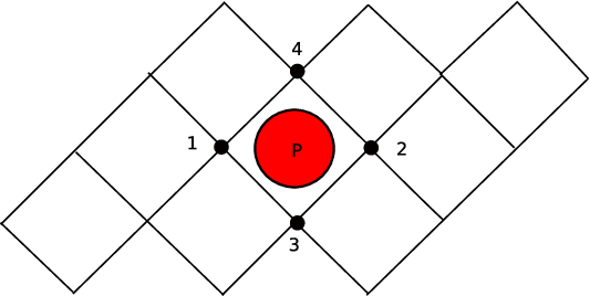
There exist two kinds of basic excitations. To label them, we have to color the plaquettes in black and white, as in a chessboard. There exist a total of three nontrivial topological charges: two of them are boson excitations, one per each violation of plaquette; and the other one is a fermion excitation. Let us recall that these boson and fermion charges are defined in the group , not the of electromagnetism. Excitations come into pairs as the end-points of string configurations. This is so when the surface is compact without boundaries.
Topological color codes (TCC) are another relevant example of topological stabilizer codes, with enhanced computational capabilities [3, 4, 5]. In particular, they allow the transversal implementation of Clifford quantum operations. The simplest lattice to construct them is a honeycomb lattice, see Fig. 2, where we place a spin- system at each vertex. There are two stabilizer operators per plaquette:
| (2.5) |
| (2.6) |

There exist six kinds of basic excitations. To label them, we first label the plaquettes with three colors: Notice that the lattice is 3-valent and has 3-colorable plaquettes. We call such lattices 2-colexes [4]. One can define color codes in any 2-colex embedded in an arbitrary surface. There exist a total of 15 nontrivial topological charges: each family of fermions is closed under fusion, and fermions from different families have trivial mutual statistics.
3. Quantum Lattice Hamiltonian with 2-Body Interactions for Color Codes
In nature, we find that interactions are usually 2-body interactions. This is because interactions between particles are mediated by exchange bosons that carry the interactions (electromagnetic, phononic, etc.) between two particles.
The problem that arises is that for topological models, like the toric codes and color codes, their Hamiltonians have many-body terms (2.4),(2.6). This could only achieved by finding some exotic quantum phase of nature, like FQHE, or by artificially engineering them somehow.
Here, we shall follow another route: try to find a 2-body Hamiltonian on a certain 2D lattice such that it exhibits the type of topological order found in toric codes and color codes. In this way, their physical implementation looks more accessible.
In fact, Kitaev [13] introduced a 2-body model in the honeycomb lattice that gives rise to an effective toric code model in one of its phases. It is a 2-body spin- model in a honeycomb lattice with one spin per vertex, and simulations based on optical lattices have been proposed [14].
The model features plaquette and strings constants of motion. Furthermore, it is exactly solvable, a property that is related to the 3-valency of the lattice where it is defined. It shows emerging free fermions in the honeycomb lattice. If a magnetic field is added, it contains a non-abelian topological phase (although not enough for universal quantum computation).
Interestingly enough, another regime of the model gives rise to a 4-body model, which is precisely an effective toric code model. A natural question arises: Can we get something similar for color codes? We give a positive answer in what follows.
3.1. The Model
It is a 2-body spin-1/2 model in a ’ruby’ lattice as shown in Fig.3. We place one spin per vertex. Links come in 3 colors, each color representing a different interaction.

| (3.1) |
For a suitable coupling regime, this model gives rise to an effective color code model. Furthermore, it exhibits new features, many of them not present in honeycomb-like models:
- •
Exact topological degeneracy in all coupling regimes ( for genus surfaces).
- •
String-net integrals of motion.
- •
Emergence of 3 families of strongly interacting fermions with semionic mutual statistics.
- •
gauge symmetry. Each family of fermions sees a different gauge subgroup.
3.2. Integrals of Motion
We can construct integrals of motion (IOM), , following a pattern of rules assigned to the vertices of the lattice, as shown in Fig.4. These rules are constructed to attach a Pauli operator of type , or to each of the vertices . The lines around the vertices, either wavy lines or direct lines, are pictured in order to join them along paths of vertices in the lattice that will ultimately translate into products of Pauli operators, which will become IOMs. Clearly, operators are distinguished from the rest. Therefore, c represent the local structure of the IOMs of our 2-body Hamiltonian (2.6). We will illustrate them with several examples of increasing complexity.

Let us start by constructing the elementary plaquette IOM as shown in Fig.5. They are denoted as . They are closed since they have not endpoints left. Using the Pauli algebra, it is immediate to check that they satisfy . Thus, there exist 2 independent IOMs per plaquette: this is the local symmetry of the model Hamiltonian (2.6).

The most general configuration that we may have is shown in Fig.6. We call them stringnets IOM since in the context of our model, they can be thought of as the stringnets introduced to characterize topological orders [15]. The key feature of these IOMs is the presence of branching points located at the blue triangles of the lattice. This is remarkable and it is absent in honeycomb 2-body models like the Kitaev model. When the sringnets IOMs are defined on a simply connected piece of lattice they are products of plaquette operators. More generally, they can be topologically non-trivial and independent of plaquette operators.

As a special case of IOM we have string configurations, i.e., paths without branching points. Some examples are shown in Fig.7. They may be open or closed, depending on whether they have endpoints or not, respectively. Strings IOM are easier to analyze. Stringnets IOM are products of strings IOM. For a given path, there exist 3 different string IOM. These are denoted as in Fig.7. Again, using Pauli algebra we get that only two of them are independent, as with the plaquette IOMs. To distinguish properly the three types we have to color the lattice. Strings are then red, green or blue. This is closely related to the topological color code [1, 2, 3].

3.3. Connection with 2-Colexes
From the previous discussion on IOMs, we have already seen a connection with the topological color codes. We can make this more quantitative. In fact, there is a regime of coupling constants in which one of the phases of the 2-body Hamiltonian reproduces the TCC many-body structure and physics.
The emergence of the topological color code is beautifully pictured in Fig.8. This corresponds to the following set of couplings in the original 2-body Hamiltonian (2.6):
| (3.2) |
This is a strong coupling limit in . Geometrically, it corresponds to shrinking the blue triangles of the original lattice into points, which will be referred as sites of a new emerging lattice, see Fig.8 (left). Recall that the blue links of these triangles represent spin-spin interactions of type. Motivated by this strong coupling limit, it is convenient to give another different coloring to the lattice which will make the transition towards the hexagonal lattice more transparent. Thus, we realize that the hexagons and vertices of the model are 3-colorable, see Fig.8 (middle): if we regard blue triangles as the sites of a new lattice, we get a honeycomb lattice, see Fig.8 (right). In fact, the model could be defined for any other 2-colex, not necessarily an hexagonal lattice.

The topological color code effectively emerges in this coupling regime. This can be seen using degenerate perturbation theory in the Green function formalism [2]. Originally, this method was applied to the Kitaev model on the honeycomb lattice [13]. Alternatively, it is possible to use the PCUTs approach (Perturbative Continuous Unitary Transformations) [16]. This is inspired by the RG method based on unitary transformation introduced by Wegner (the Similarity RG method) [17]. Originally, the PCUTs method was applied to the Kitaev model [18]. The application of this method to our model is based on mapping from the original spins on the blue triangles to hardcore bosons with spin. An operator serves to count the number of hardcore bosons by sectors. At a given perturbative order, the method produces an effective Hamiltonian such that
| (3.3) |
We are specially interested in the low-energy sector, where high-energy excitations are not present. In this sector, only effective spin degrees of freedom are relevant. Up to a constant, the effective Hamiltonian at 9th perturbative order is [1]:
| (3.4) |
| (3.5) |
This is a color code in the honeycomb lattice of effective spins! The ground state is the vortex free sector. Excitations are vortices. They are gapped and localized at plaquettes. Higher order terms are products of vortex operators. This gives rise to short-range vortex interactions.
At this point, it is illustrative to bring about an analogy with the fractional quantum Hall effect. In FQHE, the physical degrees of freedom are electrons under a very strong magnetic field perpendicular to the plane where the electrons move. The magnetic field is so strong that typically only the charge of the electrons matter, since their spins are fully polarized. Originally, the interactions among electrons are 2-body interactions: the Coulomb electric force. It is possible to write a Hamiltonian based on these interactions that describe the system from first principles. However, it is known that a better description is possible: the Laughlin wave function [19]. Despite this is an effective description of the system, it captures the whole new physics of the electronic system under these extreme circumstances. Interestingly enough, the Laughlin wave function is not an eigenstate of the original Hamiltonian based on Coulomb 2-body interactions. Instead, it is an eigenstate of a Hamiltonian with many-body interacting terms. This is the analogy. The strong coupling limit (3.2) of our model corresponds to the extreme regime of the electronic system in the FQHE. Our original 2-body Hamiltonian (3.1) is like the Coulomb Hamiltonian, while the effective topological color code Hamiltonian (3.4) with many-body terms have eigenstates which play the role of Laughlin wave functions. In fact, both systems are examples of topological orders in strongly correlated systems. However, there is a nice difference: our model retains properties of the topological color codes at a non-perturbative level because of the existence of the IOMs, which are exact in all coupling regimes.
Once we are in the phase corresponding to the topological color code, then it is possible to relate the original string and stringnets IOMs with the corresponding configurations in the color code. Thus, for example, a blue string is composed of blue links and so on and so forth. String IOMs of different color that cross once anticommute among each other. This feature is not available in honeycomb-like models. If we embed the original 2-body lattice model into a genus 1-torus, then we shall obtain a TCC in that torus. In that case, we can choose 4 independent string IOMs that form the algebra of Pauli operators on 2 qubits: , namely,
| (3.6) |
| (3.7) |
| (3.8) |
A possible choice for the configurations of these colored string operators that code the logical qubits is shown in Fig.9.

This implies an exact 4-fold degeneracy. More generally, in a surface of genus we find a -fold topological degeneracy.
4. Conclusions and Future Work
We have introduced a two-body spin-1/2 model in a ruby lattice [1, 2], see Fig.3. The model exhibits an exact topological degeneracy in all coupling regimes. Using a bosonic mapping, it is possible to discuss the emergence of strongly interacting anyonic fermions. A particular coupling regime gives rise to an effective model which is a topological color code.
We have shown that the new model exhibit enough novel interesting and relevant properties so as to justify further research. Some of these possible lines of study are as follows:
We have only studied a particular phase of the system, although we are able to study non-perturbative effects as well. The fact that all phases show a topological degeneracy anticipates a rich phase diagram. In this regard, one may explicitly brake the color symmetry that the model exhibits and still keep the features that we have discussed. It would be particularly interesting to check whether any of the phases displays non-abelian anyons. The model has many integrals of motion, although not enough to make it exactly solvable. This becomes another appealing feature of the model since other methods of study, like numerical simulations and experimental realizations will help to give a complete understanding of all its phases.
We thank the editors of this Special Issue for their kind invitation to present our written contribution for the festschrift celebrating Paolo Tombesi’s 70th birthday. MAMD also thanks the Program and the Local organizing committees for their invitation to lecture at the International Scala Conference 2009 on “Scalable Quantum Computing with Light and Atoms”. We acknowledge financial support from a PFI grant of EJ-GV, DGS grants under contracts, FIS2006-04885, and the ESF INSTANS 2005-10.
References
- [1] H. Bombin, M. Kargarian, M.A. Martin-Delgado, “Interacting Anyonic Fermions in a Two-Body ‘Color Code’ Model”; arXiv:0811.0911.
- [2] M. Kargarian, H. Bombin, M.A. Martin-Delgado; “Topological Color Codes and Two-Body Quantum Lattice Hamiltonians”; Submitted to the Special Issue on ”Quantum Information and Many-Body Theory”, New Journal of Physics. Editors: M.B. Plenio, J. Eisert; arXiv:0906.4127.
- [3] H. Bombin, M.A. Martin-Delgado; “Topological Quantum Distillation”; Phys. Rev. Lett. 97, 180501 (2006). quant-ph/0605138.
- [4] H. Bombin, M.A. Martin-Delgado “Exact Topological Quantum Order in D=3 and Beyond: Branyons and Brane-Net Condensates”; Phys. Rev. B 75, 075103 (2007); cond-mat/0607736.
- [5] H. Bombin, M.A. Martin-Delgado; “Topological Computation without Braiding”; Phys. Rev. Lett. 98, 160502 (2007); quant-ph/0610024.
- [6] X.G. Wen, Quantum Field Theory of Many-body Systems: From the Origin of Sound to an Origin of Light and Electrons (Oxford Univ. Press, New York, 2004).
- [7] X.G. Wen, “Topological orders and edge excitations in fractional quantum Hall states”; Adv. Phys., 44, 405 (1995).
- [8] A. Micheli, G.K. Brennen, P. Zoller, “A toolbox for lattice spin models with polar molecules”; Nat. Phys. 2, 341 (2006). quant-ph/0512222.
- [9] L. Jiang, G.K. Brennen, A.V. Gorshkov, K. Hammerer, M. Hafezi, E. Demler, M.D. Lukin, P. Zoller, “Anyonic interferometry and protected memories in atomic spin lattices”; Nat. Phys. 4, 482 (2008). arXiv:0711.1365.
- [10] M. Lewenstein, A. Sanpera, V. Ahufinger, B. Damski, A. Sen, U. Sen, “Ultracold atomic gases in optical lattices: mimicking condensed matter physics and beyond”; Adv. Phys. 56, 243 (2007).
- [11] D. Gottesman, “Class of quantum error-correcting codes saturating the quantum Hamming bound”. Phys. Rev. A 54, 1862 (1996).
- [12] A. Yu. Kitaev, “Fault-tolerant quantum computation by anyons”, Annals of Physics 303, 2–30 (2003), quant-ph/9707021.
- [13] A. Yu. Kitaev; “Anyons in an exactly solved model and beyond”; Ann. of Phys. 321, 2–111 (2006). arXiv:cond-mat/0506438v3.
- [14] L.-M. Duan, E. Demler, M.D. Lukin, “Controlling Spin Exchange Interactions of Ultracold Atoms in Optical Lattices”; Phys. Rev. Lett. 91, 090402 (2003). arXiv:cond-mat/0210564.
- [15] M. Levin, X.-G. Wen, “String-net condensation: A physical mechanism for topological phases”. Phys. Rev. B 71, 045110 (2005).
- [16] C. Knetter, G. Uhrig; “Perturbation theory by flow equations: dimerized and frustrated S = 1/2 chain”; Eur. Phys. J. B13, 209 (2000).
- [17] F. Wegner, “Flow-equations for Hamiltonians”; Ann. der Phys. 506, 77 (1994).
- [18] J. Vidal, K.P. Schmidt, S. Dusuel; “Perturbative approach to an exactly solved problem: Kitaev honeycomb model”; Phys. Rev. B 78, 245121 (2008). arXiv:0809.1553v1.
- [19] R.B. Laughlin, “Anomalous quantum Hall effect - An incompressible quantum fluid with fractionally charged excitations”; Phys. Rev. Lett. 50, 1395 (1983).