Statistical mechanics of LDPC codes on channels with memory

A common problem in modern mobile telecommunication systems is that the strength of the signal varies over time as a result of e.g. the motion of the receiver with respect to the source and the varying number of obstacles that shadow the signal over time. Channels describing communication of attenuated signals are termed ‘fading channels’. Fading channels are modeled by finite-state Markov channels (FSMC) [1]. These channels have fueled significant research activity (for a recent review on the subject see [2]). In FSMCs there exist a number of different channel states that correspond to the various possible attenuation factors. Each of the states describes a memoryless channel characterized by an error probability, while, the transition from one state to another occurs according to a stationary Markov process. Since there are different states in the FMSC the error-probabilities between subsequent uses of the channel are correlated, i.e. there is memory in the channel.

One of the central problems in the domain of error-correcting codes is the design of codes that reach Shannon’s limit. The gap between the Shannon limit and the computational limit was closed by turbo codes [3] and by low-density parity-check codes (LDPC) [5, 4]. For erasure channels it was shown that LDPC can reach the Shannon capacity [6] while for general symmetric channels one can approach the Shannon limit [7]. To design capacity approaching LDPC-codes one uses the density evolution (DE) equations to determine the decoding thresholds [8]. Since channels with memory have a higher capacity [9, 10] one would like to introduce memory in the decoding process. Important therefore are the extensions of turbo codes and LDPC codes to FSMCs [11, 12].

Statistical physics has entered the stage of error correcting codes after the discovery that the decoding problem describing interactions between parity checks and codeword variables can be mapped to large frustrated systems of interacting particles [13]. Since then, physicists have analyzed the performance of Gallager, MacKay-Neal and Turbo codes over binary-symmetric, -asymmetric, or real-valued channels [14, 15, 16, 17, 18] (for a review see [19]). The main actor in this approach is the generating function of the a posteriori probability distribution of codewords. This is similar to the free energy of spin models. Using the replica method one derives directly the so-called density evolution equations [8] from the free energy. Moreover the tools of statistical mechanics can be used to calculate the error-exponents [20, 21], MAP-thresholds [22] and modified schemes of belief-propagation using replica symmetry-breaking effects [23]. Generally, the lion’s share of the volume of research on error-correcting codes has been dedicated to memoryless channels. Apart from the work of [24], channels with memory, or any other FSMC models, have never been to our knowledge analyzed within statistical physics.

Our work is based on techniques that were developed to analyze macroscopic properties of ‘small-world’ networks. These systems, due to their close relation with real-world networks, have been the subject of intense study from a variety of scientific disciplines [25, 26, 27]. Small-world lattices have a particular architecture that allows both a high clustering coefficient and a small shortest path-length (unlike the random Erdös-Renyi graphs). They are constructed by superimposing random and sparse graphs with a finite average connectivity onto a one-dimensional ring. An exact analysis of the thermodynamic properties of such systems can be found in [28]. As it is, FSMCs can be mapped to small-world lattices, whereby messages between parity checks and codeword-nodes propagate along the sparse graph while messages between channel-state nodes propagate along the one-dimensional chain.

In this letter, we present a general method to derive the density evolution equations for symmetric or asymmetric FSMCs. This includes an exact analysis of the Gilbert-Elliot channel (GEC) [29, 30]. Fully asymmetric cases could be used to describe burst errors in VLSI circuits [31, 32]. We compute the decoding thresholds for the different channels. For symmetric FSMCs we compare the results to [12] while for memoryless channels to [33, 18].

Let us now be more particular. A signal $\mbox{\boldmath$\sigma$}^{0}\in\{-1,1\}^{N}$, prior to its communication over the channel, is encoded to $\mbox{\boldmath$\sigma$}\in\{-1,1\}^{M}$ with $M>N$. The set of codewords $\mathcal{C}$ of an LDPC-code is defined by its parity check matrix $\mathbb{H}$ through: $\mathcal{C}=\{\mbox{\boldmath$\sigma$}\in\{-1,1\}^{M}|\mathbb{H}\ast\mbox{\boldmath$\sigma$}=1\}$ with $(\mathbb{H}\ast\mbox{\boldmath$\sigma$})_{i}=\prod_{j=1}^{M}\sigma_{j}^{\mathbb{H}_{ij}}$ for all $i=1,\ldots,M-N$. For $(C,K)$-regular LDPC-codes the parity check matrices are random, sparse matrices of dimension $(M-N)\times M$ with $\mathbb{H}_{ij}\in\{0,1\}$ and with $K$ non-zero elements per row and $C$ non-zero elements per column.

Channel noise can be modeled with the transformation $\mbox{\boldmath$\sigma$}\to\mbox{\boldmath$\rho$}$ where the output of the channel $\mbox{\boldmath$\rho$}\in\{-1,1\}^{M}$ depends on the input through the state variable $\mbox{\boldmath$s$}\in\mathcal{S}^{M}$:

The probability of the states $P_{\rm state}(\mbox{\boldmath$s$})$ follows a Markov process

We will denote by $\mbox{\boldmath$\sigma$}^{0},\mbox{\boldmath$s$}^{0}\in\{-1,1\}^{M}$ the true codeword and true channel state vectors respectively that were realized during the signal communication. Depending on the definition of the Markov process and the channel noise one has different FSMCs. The derivation of the DE equations stays mainly the same. We consider two-state Markov-modulated binary channels. For these channels the noise is a random variable drawn from the distribution

The channel can be in two states: $\mathcal{S}=\left\{G,B\right\}$. Since we take $(p_{B}+q_{B})>(p_{G}+q_{G})$, $B$ is called the bad state and $G$ is called the good state. The Markov process is determined by the transition probability $\mathcal{W}$ given by

with $g$ the transition probability from state $B$ to $G$ and $b$ the transition probability from state $G$ to $B$ (fig. 1). We define the memory $\mu_{\ell}$ at time step $\ell$ of the Markov process as

From (2) we find $\mu_{\ell}=\left(1-g-b\right)^{\ell}\equiv\mu^{\ell}$ with the time index $\ell=1,2,\ldots$ and $\mu\in[-1,1]$. For $\mu>0$ we have persistent memory: the probability of remaining in a given state is higher than the steady-state probability of being in that state. For $\mu<0$ we have an oscillatory memory. We also define the good-to-bad ratio $\rho=\frac{g}{b}$. The FSMCs we consider are determined by the 6-tuple $\mathcal{T}=(\mu,\rho,p_{B},q_{B},p_{G},q_{G})$. The GEC [29, 30] corresponds to the subset of channels $\mathcal{T}_{\rm{GEC}}=(\mu,\rho,p_{B},p_{B},p_{G},p_{G})$. We will also consider channels $\mathcal{T}_{\rm{AS}}=(\mu,\rho,\kappa q_{B},q_{B},\kappa q_{G},q_{G})$ with $\kappa\in[0,1]$ and $\mathcal{T}_{\rm{Z}}=(\mu,\rho,0,q,q,0)$. The latter channel could be useful for modeling blocks of bad memory or bursts of unidirectional noise in VLSI circuits.

The starting point for the derivation of the DE equations is the calculation of the generating function $f$ of the a posteriori probability distribution of the codeword $\sigma$ given the channel’s output $\rho$ and the parity check matrix $\mathbb{H}$:

Using Bayes’ law and (1) we obtain

with $P(\mbox{\boldmath$\sigma$}|\mathbb{H})$ the initial probability distribution of the codewords and $Z$ a normalisation constant. We will consider unbiased sources of i.i.d.r.v: $p_{\rm init}(\mbox{\boldmath$\sigma$})=2^{-M}$. $P_{\rm chan}(\mbox{\boldmath$\rho$}|\mbox{\boldmath$s$},\mbox{\boldmath$\sigma$})$ gives the a priori probability distribution of the output $\rho$ given the state vector $s$ and the codeword $\sigma$ (2). The Kronecker delta constrains the summation only to those codewords that obey the parity check equation.

Averaging the generating function over the ensemble of parity-check matrices, true-states, true-codewords and outputs gives

plus irrelevant constant terms. The probability distribution of the parity-check matrices $P(\mathbb{H})$ of a $(C,K)$-regular code can be written in terms of a tensor with $K$ indices and elements in $\{0,1\}$, such that the probability that an element of the tensor is 1 is $C\frac{(K-1)!}{M^{K-1}}$ and the sum of the elements equals $C$ for all of its indices (see e.g. [19, 18]). The free energy $\overline{f}$ can then be calculated using the replica trick $\langle\log Z\rangle=\lim_{n\to 0}\frac{1}{n}\log\langle{Z^{n}}\rangle$. This results, for $M\rightarrow\infty$, in a saddle point integral. The free energy at the saddle point is given by

with $\Psi$ the exponent of the saddle point integral. The extremization is taken over the order parameter functions $P(\mbox{\boldmath$\sigma$},\sigma)$ and $\hat{P}(\mbox{\boldmath$\sigma$},\sigma)$. These represent the usual order parameter functions describing finite connectivity systems, see for instance [34], with $\mbox{\boldmath$\sigma$}=(\sigma^{1},\ldots,\sigma^{n})\in\{-1,1\}^{n}$ originating from the replication of the dynamic codeword-variables while $\sigma\in\{-1,1\}$ stems from the inclusion of the quenched true codeword in the order function.

The exponent $\Psi$ reaches a minimum at the values $\left(P(\mbox{\boldmath$\sigma$},\sigma),\hat{P}(\mbox{\boldmath$\sigma$},\sigma)\right)$ that satisfy the saddle point equations:

where we defined

and we introduced the average $\langle\cdot\rangle_{\rho|s^{0},\tau}$ over $P_{\rm{chan}}(\rho|s^{0},\tau)$. Note that while the summations over the replicated codeword variables $\left\{\mbox{\boldmath$\sigma$}_{i}\right\}_{i=1\ldots N}$ have been performed by reducing the graph into a single-site problem, the summations over the replicated channel-state variables $\left\{\mbox{\boldmath$s$}_{i}\right\}_{i=1\dots N}$ is written as a trace over matrix products in (16). This constitutes the key difficulty in our problem as we are dealing with the $(2^{n}+1)\times(2^{n}+1)$ replicated transfer matrix:

To proceed further we now have to make an assumption with regards to the structure of the replica space. The simplest, replica symmetric ansatz, assumes that

for some densities $W,Z$. For the left- and right-eigenvectors $L(\mbox{\boldmath$s$},s)$, $R(\mbox{\boldmath$s$},s)$ of $V$ we now assume

The form of the above two equations follows the central assumption of [28, 35]. It allows us to take the remaining trace in (16). All distributions above are normalized at $n\rightarrow 0$. The densities $\mathcal{P}_{R}$ and $\mathcal{P}_{L}$ represent respectively the right- and left- eigenvectors of $\mathcal{W}$:

Following similar computations as in [28, 36], we derive in the limit $n\to 0$ the closed, self-consistent equations

and also

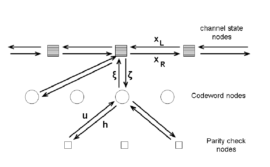
Equations (24-29) are the DE equations for the binary asymmetric two-state Markov channel. They describe the evolution of the densities of messages propagating along a tripartite graph. The graph consists of a chain of channel-state nodes connected to codeword nodes and these in turn to parity check ones. This graphical representation of the decoding process corresponds to an efficient algorithm [38], equivalent to the sum-product algorithm used in channels without memory. The tripartite graph has three different sets of vertices: the set $V_{\rm code}$ of codeword nodes, the set $V_{\rm pc}$ of parity check nodes and the set $V_{\rm chan}$ of channel-state nodes, see fig. 2. Due to the presence of memory there are 6 types of messages propagating according to:

The update equations for single-graph instances for these messages (the so-called ‘message-passing’ equations) [38] correspond to the functions within the delta functions in the DE equations (24-29).

We are interested in deriving the critical noise levels beyond which decoding is not possible. This information can be obtained through the observable $\rho_{\sigma}\equiv\frac{1}{|I_{\sigma}|}\sum_{i\in I_{\sigma}}\sigma_{i}=\int dh\tilde{W}(h|\sigma){\rm sign}(h)$ where $I_{\sigma}$ describes the sublattice $I_{\sigma}=\{i\in V_{\rm code}|\sigma_{i}^{0}=\sigma\}$ and $\tilde{W}$ the distribution of the marginals of the decoding variables

The value $\rho_{\sigma}=1$ corresponds to perfect decoding (ferromagnetic phase) while $\rho_{\sigma}<1$ describes decoding failure (paramagnetic phase). We detect the transition by numerically solving the DE equations (e.g. through population dynamics [37]).

The decoding thresholds in the parameter space $\big(\frac{1}{2}(p_{G}+q_{G}),\frac{1}{2}(p_{B}+q_{B})\big)$ for a Gallager $(C,K)=(3,4)$ code on a $\mathcal{T}_{\rm AS}$-channel are shown in fig. 3. Dotted lines separate ferro- from paramagnetic solutions for memoryless channels with $\mu=0$, while symbols correspond to channels with memory for $\mu=0.9$. We show four degrees of channel asymmetry characterized by the variable $\kappa=p_{B}/q_{B}=p_{G}/q_{G}$. Note that to simplify the presentation of our results the two channel states have here the same $\kappa$. The decoding thresholds for $\kappa=0$ are computed from the DE equations for $\kappa\rightarrow 0$, which can be derived when rescaling the fields $h\rightarrow\beta h$, $u\rightarrow\beta u$, $\zeta\rightarrow\beta\zeta$ and $\xi\rightarrow\beta\xi$ with $\beta=-\frac{1}{4}\log(\kappa)$. The points marked by the star-symbols correspond to the points where the two channel states have the same error probability, $p_{B}=p_{G}$ and are taken from [18]. Beyond the star-symbol (lower-right part of the fig.) the roles of the ‘good’ versus the ‘bad’ channel are interchanged. In this fig. we also see that both the presence of memory and that of asymmetry in the channel allows for higher noise levels. In the limiting cases of $\kappa=1$ our results agree very well with those of [12]. In table 1 we give the decoding thresholds corresponding to fig. 3.

In fig. 4 we present results from the channel $\mathcal{T}_{Z}$ in which there exist two Z-type states: $(p_{B},q_{B})=(0,q)$ and $(p_{G},q_{G})=(q,0)$ (hence the terms ‘good’ vs ‘bad’ are not very meaningful here). This type of configuration can model ‘burst-error’ channels where a very large number of consecutive bits appear corrupted while the corruption is selective with regards to the input symbol. We show results in the $(\mu,q)$ space for Gallager $(C,K)=(3,4)$ and $(4,6)$ codes. The lower dashed line corresponds to the noise level $2q_{{\rm BSC}}$ where $q_{{\rm BSC}}$ is the critical level of the memoryless binary-symmetric channel. The fact that the marker at $\mu=0$ coincides with the dashed line is not a coincidence since in this limit the channel has two complementary Z-type states without memory, and therefore, with an equal transition probability between them. The upper dashed line corresponds to the critical noise level of a memoryless Z-channel [18]. At $\mu=-1$ the transition probabilities become $b=g=1$ and thus the channel oscillates between the two states. We note that this fig. is symmetric with respect to the $\mu=0$ axis; a property that also follows from the DE equations.

Error-correcting codes on channels with memory are known to outperform the traditional ones on memoryless channels. They can be used in modern mobile communication systems or to model burst-error channels. In this letter we have presented a technique for deriving the density evolution equations for multi-state channels. This method is based on the diagonalisation of replicated transfer matrices that was originally developed to study ‘small-world’ systems. It turns out that the representation of the LDPC multi-state decoding problem on graphs shares a common architecture with ‘small-world’ systems: In memoryless channels, decoding occurs with message-passing between symbol variables (the ‘spins’) which are connected to parity-check variables (the ‘couplings’). Channels with memory introduce a new element to this hypergraph which can be seen and treated as a chain of channel-state variables with nearest-neighbor interactions.

We have presented results for the Gilbert-Elliott channel and its generalisation to asymmetric two-state channels with memory. The density evolution equations that follow from the analysis reproduce very well the special limiting cases of the GEC or the memoryless binary-asymmetric channel. The method can be applied to a variety of multi-state error-correcting codes, such as multi-symbol, gaussian-, non-Markovian or intersymbol-interference channels. From a statistical physics point of view an interesting future direction would be the inclusion of replica symmetry-breaking effects [39] which might correct the critical noise levels we present here.