Higher order corrections to Heterotic M-theory inflation
Abstract
We investigate inflation driven by dynamical five-branes in Heterotic M-theory using the scalar potential derived from the open membrane instanton sector. At leading order the resulting theory can be mapped to power law inflation, however more generally one may expect higher order corrections to be important. We consider a simple class of such corrections, which imposes tight bounds on the number of branes required for inflation.
I Introduction
There has been a significant effort in recent years to better understand moduli stabilisation and cosmological dynamics in a specific class of string theory models. More precisely, whilst much of this effort has been focused on the type IIB superstring, there has been significant progress in the strongly coupled Heterotic models which are conjectured to be the low energy limit of Heterotic M-theory [1, 2]. These models are phenomenologically interesting because of the gauge group which comprises a visible sector (including the standard model) and hidden sector. The embedding of wrapped five-branes in this setting was investigated and suggested as an ideal method of driving inflationary cosmological scenarios [3, 4, 5, 6, 7]. The fact that it naturally contains a dark sector, which is coupled gravitationally to the visible sector, suggests a natural place to localise dark matter making such models phenomenologically relevant. With the advent of flux compactification, various groups tried to develop more realistic models of the vacuum structure of the theory [8, 9, 10, 11] which led to the embedding of a standard model-like sector [12] into the Heterotic theory using the vector-bundle moduli.
Inflationary model building in the Heterotic model [13, 14] was supported by precision data retrieved from WMAP. This culminated in the multi-brane model of [15] (supplemented by follow-up work in [16, 17]) and other related ideas [18]. The important point about [15] is that it provided a concrete embedding of assisted inflation [19, 20, 21, 22] into a fully UV-complete theory, where the inflationary phase occurs before the end of moduli stabilisation. Assisted inflation works for theories with steep scalar potentials, provided that there are multiple scalar fields following similar trajectories through field-space. The combined effect of the multiple fields acts to enhance the Hubble friction term in the field equations, thus allowing sufficient inflation to occur. In this framework, the scalar potential can be significantly steep to ensure that the dynamics of the geometric moduli can be ignored, therefore indicating that assisted inflation would be the most likely possibility for driving inflation in this model. We also note that the end of inflation is naturally understood to occur through the tunneling of branes into the orbifold planes via instanton transition into the boundary, see [30, 31] for some related work. After inflation, the remaining moduli can be stabilised in a de-Sitter vacuum [32, 33, 34] which is well controlled due to the known higher derivative corrections [35]. Unfortunately stabilising the more general structure case is still a work in progress, although it is likely that including gaugino condensation and following the proposals [36, 37] will achieve this.
The model of assisted inflation arises very naturally in this instance by considering only the leading order terms in the superpotential [15]. A natural question to ask then relates to whether inflation is spoilt through the inclusion of higher order terms, since this would indicate another (potentially un-natural) source of fine tuning. We aim to go beyond the expansion by considering additional corrections to the tree-level superpotential, as loop corrections are difficult to calculate explicitly, to further explore the allowed inflationary parameter space. Our naive expectation is that these corrections will impose tighter constraints on the background parameters in order for inflation to occur - however since the scalar potential is comprised solely of exponential terms we anticipate that inflation (if it occurs) could be eternal. To check this assumption it is useful to study the phase space in order to find attractor solutions.
The organization of this note is as follows. In section II we introduce the relevant M-theory background required for model building. We follow this in section III by discussing assisted inflation, and how it is realized in this theory. In sections IV, V and VI we explore and explain how this setting can be made more accurate through several new additional elements. The main contribution of this paper is in providing and discussing the cosmological implications of these elements, which are higher order corrections to the inflationary potential, and discuss how they further restrict the inflationary parameter space.
II The M-theory background
Let us consider the model of the strongly coupled Heterotic string on the orbifold , where there are two ’end of the world’ branes localised at the fixed points of the orbifold action [1, 2]. For simplicity we will consider a simplified model, whereby we restrict ourselves to a sector where , and where there are five-branes wrapping an isolated genus-zero curve in the , localised along the orbifold direction. The superpotential for the theory takes the following form [15]
| (1) |
where we have defined each of the contributions to be
| (2) | |||||
in terms of chiral superfields. Note that is a parameter fixed by the UV-cutoff of the gauge group of the hidden theory, is the normalised coupling of the five-branes, whilst is given by the normalised integral of the Kähler form over the relevant two-cycle. Let us briefly comment on some of the notation here, since it is different to that employed in the type II case. Firstly, it is the superfield that controls the overall volume of the compact . The superfield measures the length of the orbifold, and is the superfield associated with the location of the fivebrane along this interval. Strictly speaking each of these superfields contains axionic contributions associated with the reduction of the three-form flux along the orbifold direction
| (3) | |||||
| (4) | |||||
| (5) |
Clearly measures the distance of the th brane from the visible sector, therefore . We also have contributions from open-membranes wrapping cycles within the , which have an averaged volume given by . These open-membrane contributions can be interpreted as a shift in the volume of the internal space and have phenomenological values , whilst typically . We will often refer to ’canonical values’ for these parameters which are as an approximate solution [15], and therefore we can, in principle, write the superfields solely as functions of . Of course if the hidden sector gauge group is no longer , then the dual Coxeter number is different and one obtains different values for these parameters, eg , if the group is [11]. Also note that refers to the axionic component of each of the superfields.
In the flux superpotential (2) is the three-form flux which is to be integrated over the manifold, and is the usual form. The presence of this term is crucial in order to stabilise the complex structure of the Calabi-Yau manifold. The gaugino condensate contribution () contains various parameters proportional to the Coxeter number of the condensing gauge group - and various other integer terms parameterised by the functions which arise from integrating the Kahler form over the corresponding internal cycles. As in the case of type II string theory, this term plays a vital role in the stabilisation of the compact space.
The open membrane contribution () arises from Euclidean membranes fully wrapping cycles within the . The various terms correspond to instantons between the visible sector and the brane, the brane and the hidden sector and the visible and hidden sectors respectively. The prefactor is the Pfaffian associated with the hidden sector. It is typically a function of the vector bundle moduli living on the hidden sector domain wall - however we will ignore these in our toy model construction, although they play a vital role in realising models of the MSSM. It is this superpotential contribution which will be the relevant one for inflationary model building.
Having specified the superpotential, we must also consider the Kahler potential for the theory which (as in the type II case) is separable at tree level
| (6) | |||||
where corresponds to the potential on the complex structure moduli space. It will usually be simpler to introduce the function
| (7) |
to reduce the expressions above. For simplicity we will stabilise the complex structure at high scales allowing us to integrate them out of the theory. Also note that (for completeness) we have included the presence of the leading order correction to the theory coming from the terms in the eleven dimensional action, denoted by , which is a function of the Euler number of the and is therefore a topological restriction. We will set it to be zero for the time being.
The second term in (6) should be familiar from the type II theory, and is explicitly a function of the Kahler moduli only. Since we have assumed that there is only a single modulus in this sector, the intersection numbers become trivial. Extending this to the multi-moduli case is technically more complicated, although can be done in principle.
III Fivebrane inflation
Having set up the relevant background, one can now describe how fivebrane inflation works in this set-up [13, 14, 15]. Modular inflation driven by either the geometric moduli themselves [23, 24, 25, 26], or their axionic partners has previously been considered in the literature [27, 28, 29]. In this paper we are interested in inflation driven by the dynamics of five-branes along the orbifold length, which is the M-theory counterpart of -brane inflation [38]. In order to proceed, one must have parameteric control over the theory. In particular this usually means stabilising all the moduli of the compactification prior to the inflationary phase. This is still a non-trivial task in the heterotic context. Fortunately the presence of multiple branes wrapping genus zero curves, allows us to by-pass this condition (at least for the purposes of inflationary model building). It turns out that the scalar potential is actually steepest along the five-brane directions, which leads to the possibility of inflation occuring before the stabilisation of the (pseudo)moduli - where the inflaton direction is identified with the steepest part of the potential [15].
Standard slow roll inflation relies on the fact that the inflaton potential is extremely flat, therefore the acceleration of the inflaton field can be neglected - at least for early times - and the universe will undergo sufficient expansion. However a scalar potential that is exponentially decreasing is always too steep for a sustained period of cosmological inflation in this context. The inflaton undergoes rapid acceleration and the slow roll approximation rapidly breaks down. One simple way to alleviate this problem is to consider not just a single field for the inflaton, but several fields that all have the same trajectory. The combined effect of these fields is to increase the strength of the Hubble term in the inflaton equation of motion, which acts much like a friction term. The more fields we can include, the more the motion will be damped because the friction is increasing. This was given the name assisted inflation in the literature.
The model of assisted inflation we describe herein, actually belongs to a special class of models which overlap between assisted inflation and power law inflation - so called because the scale factor expands like . In terms of an effective description, it is more useful to parameterize power law inflation through the introduction of an exponential potential of the form
| (8) |
(where we work in Planckian units) with corresponding to a canonical scalar field. The resulting slow roll parameters can be seen to reduce to constants. We find that , and therefore since inflation demands we simply need to ensure that for inflation to occur. One potential difficulty with these solutions is that there is no natural exit from inflation, since the relevant parameters are constants - therefore some other mechanism must be invoked to end power law inflation.
Returning to the case at hand, we include five-branes, wrapping two-cycles within the compact space which are constrained to move along the orbifold direction, and fill the large dimensional space-time. Let us briefly discuss some of the technical aspects associated with such a construction. Firstly we will take the Horava-Witten model, which assumes that the seven-dimensional compact space is simply the product orbifold , where the is a manifold with holonomy. More generally one should consider compactifications on full holonomy manifolds, or orbifolds where is a manifold of structure. Thus our choice of background is already subject to some tuning of the initial conditions, in that we are selecting a specific compactification manifold from the space of all such manifolds. It may well turn out that the compactification is the more dynamically favoured one. However in the absence of a fuller understanding of M-theory we must include this as part of our initial conditions. Having specified our compact space we must then be careful to wrap the five-branes only along genus zero curves, since terms arising from branes wrapped on higher genus curves will vanish due to holomorphy and therefore will not contribute to the theory. Finally we will assume that the fivebranes wrap these cycles only once - as this simplifies things considerably since the anomaly cancellation expression then reduces to
| (9) |
where are integer coefficients arising from the second Chern-Classes on the visible/hidden boundary respectively.
Given these constraints we find that the superpotential is dominated by terms coming from the open-membrane instantons
| (10) |
with the Kahler potential given as in (6). It was then argued in [15] that the initial conditions require the five-branes to be localised in the middle of the orbifold, where the total orbifold length is much larger than the other scales in the theory. This ensured that the first three terms in the superpotential can be neglected as being exponentially suppressed. This then leaves only the term arising from interactions between each of the five-branes
| (11) |
It is a standard result in supergravity that the scalar potential is minimised at supersymmetric vacua where , with running over the various moduli in the theory. Therefore it is energetically favourable for us to set . With this assumption we find the constraint
| (12) |
where is the full Kahler potential. Neglecting the complex structure term then amounts to trying to solve the expression
| (13) |
which is generally very difficult to do analytically.
Consequently in [15] they opt to take a simpler route, namely to individually set each term in the covariant derivative to zero - i.e. they impose
| (14) |
In more detail this can be summarised as:
- •
The first constraint basically tells us that the superpotential is independent of each of the individual superfields. The only way for this to be non-trivially satisfied (i.e not having a vanishing superpotential) is for to be a constant. This is therefore a geometrical condition since it implies that the five-branes should be equidistant from each other.
- •
The secondary constraint is that which reduces to
(15) which is assumed to be true for sufficiently large values of .
- •
The final assumption was to keep only nearest-neighbour instantons contribute to the superpotential. Defining the quantity one sees that the superpotential reduces to
(16) which scales linearly with , and therefore is the leading term in a expansion.
Given the above assumptions the F-term scalar potential can be seen to schematically reduce (at leading order) to the form
| (17) |
where the superpotential term is a strictly decaying exponential contribution. This exponential suppression of the inflaton constitutes the dominant mechanism for building concrete inflationary models within superstring theory11 1 For example in the context of type II theory we see that the inflaton potential is of the form , where is related to one of the Kahler moduli in the large-volume models in IIB, or one of the complex structure moduli in the weakly-coupled models of type IIA. The main difference between these approaches and the one in the heterotic theory are to do with moduli stabilisation. The models of the type II theory have all their (heavy geometric) moduli stabilised initially at some high scale allowing inflation to occur through the dynamics of the lightest moduli, whilst in the heterotic M-theory model; none of the moduli are stabilised prior to inflation. In the type II context, most of the moduli have already been stabilised assuming zero temperature and therefore simply turning on finite temperature effects may not be completely consistent since this may have the effect of shifting the vev’s of the fields - potentially destroying the nice inflationary and phenomenological properties of such models..
Now since the branes are assumed to be equidistant, one can use their combined centre of mass to re-write the superpotential in terms of a canonical field . In terms of which we see that the superpotential becomes
| (18) |
where is a function of the other geometric moduli via . Note that our conventions differ from that in [15] thus accounting for the change in the definition of the parameter, but are still associated with the real parts of the superfields as in eqn (3-5). Using the definition of the scalar potential above we see that the inflaton F-term potential for is in fact
| (19) |
where it was assumed that are approximately constant during inflation. One can check that the potential along the inflaton direction is still actually the steepest potential in field space, despite the apparent dependence on the orbifold modulus.
It is straight-forward to see that this exponential potential can then be mapped to that of the power law form and we then obtain power law inflation. In this case there is also a natural mechanism for the end of inflation, since eventually the orbifold length will grow larger and then induce gaugino condensation on the hidden boundary. The remaining terms in the superpotential will then be non-negligible and also contribute to the F-term scalar potential. The combination of higher order instanton effects and gaugino condensation should then stabilise all the remaining geometric moduli. Before proceeding, let us stress that the above model works precisely because we assume the geometric moduli can be taken to be approximately constant during the inflationary phase driven by the exponentially decaying inflaton. In addition the assumption that all the branes are localised near is crucial in obtaining the simple form for the scalar potential
In the remainder of this paper we will describe how the setting above can be further elaborated by means of additional elements present in the theory, which have not yet been fully explored.
IV Constraining
Let us appraise how all the assumptions above affect the bounds on the number of branes. One of the interesting features of this model is that is bounded from both above and below [15] if one searches for inflating trajectories. Indeed at leading order the scalar index is related to the number of branes and therefore one can use the WMAP normalisation to cherry-pick the requisite solution. Rather than consider the inflationary normalisation, let us instead see how the causal structure of the theory imposes constraints on . Recall that a major simplifying assumption in the derivation of the F-term potential (19) was that we assumed , which is a significantly stronger bound than simply assuming which comes from the reality of the Kahler potential. We will be more careful than this and examine the full constraint here.
Firstly let us consider the situation at the very start of inflation. The initial distribution of branes is assumed to be localised around the middle of the orbifold, therefore we have and thus once we set the axions all to zero. Since we must demand that for the Kahler potential to be well defined, this immediately yields the initial upper bound that
| (20) |
where we have included the term coming from the corrections for generality. Setting initially, and fixing and to be constant - which we assume will be typical values of the parameters at this time - we see that as an order of magnitude approximation. However if we wish to consider a more realistic bound then we must recall that is also a linear function of , and therefore does not provide a useful bound on . We can however bound the size of the correction term , which must satisfy
| (21) |
where we remind the reader that is the averaged volume of the Calabi-Yau. Since is a function of the Euler number of the particular manifold this in turn imposes a constraint on the number of complex structure and Kahler moduli i.e this is a geometric condition.
Regarding the inflationary bound on , recall that for power law inflation to work, we must decouple the higher order dependence from the scalar potential which requires the following condition to be satisfied (from a detailed analysis of the scalar potential)
| (22) |
If we make the usual assumption regarding inflation occuring when the branes are near the middle of the orbifold then we can rewrite this constraint as
| (23) |
As far as phenomenological implications go, the constraint equation above can be interpreted as constraining the solution space for fixed volumes. The corresponding phase space can be seen to be concave near indicating that the constraint is more easily satisfied for larger values of (for a given choice of volume).
The reality condition on the parameter can then be imposed. Since there is no problem for we will only focus on compactifications which have or as these are the two most interesting cases.
Let us begin with the former condition, where we find the constraint equation can be written as and demanding positivity of is equivalent to the condition
| (24) |
Since we must assume the validity of the supergravity approximation we require large volumes, and therefore the constraint is satisfied for all values of despite the term on the left hand side not being a monotonic function.
If one assumes that is sufficiently large, then the leading term in (24) imposes a bound on
| (25) |
thus providing a constraint on the number of five-branes. In fact this full bound is a little tighter than the one considered in [15] using the standardised assumption that and since we find that is constrained viz .
Now let us consider the limit , where the constraint equation simplifies considerably. In fact the relevant positivity condition reduce to which is satisfied for all values of and therefore does not constrain the number of five-branes. Of course one must be careful with the physical interpretation of this result because the Kahler potential is actually no longer well defined in this limit.
Another immediate limitation of the setting in [15] is related to the vanishing of the five-brane F-terms. We recall that this meant setting and in the covariant derivative. The first constraint is actually remarkably robust and would seem to be the simplest choice possible. However the second constraint requires the first derivative of the Kahler potential along the direction to vanish at large volume. Whilst this is an adequate assumption, one must be careful to check that this is consistent with the functional form of the scalar potential. In other words, if we drop these terms, then we cannot keep terms of the same order arising from the other F-terms. Indeed all of the (first) Kahler derivatives will have terms of order and so on its own is not a consistent approximation.
Relaxing this assumption makes things slightly more complicated as there are now off-diagonal pieces contributing to the inverse Kahler metric on field space. Fortunately all the F-terms are independent of the superpotential, and therefore one only needs to study the Kahler potential. After a laborious calculation, and assuming that is dominated by the volume factor as before, we find that the relevant constraint to decouple the additional dependence becomes
| (26) |
which can easily be satisfied for a range of . Note that this is a weaker bound than the one obtained by studying the decoupled inflaton mode and therefore we will not study it further.
V Dissolving branes
The results presented in [15] can be further re-interpreted as follows. An interesting issue, not yet fully explored, relates to the growing size of the orbifold. Recall that the basic theory of instanton inflation here relies on the fact that inflation happens rapidly, well before the five-branes move far from their initial positions. It is expected that power law inflation will naturally self-terminate once the (initially) subleading instanton terms become comparable to those associated with the inflaton sector. Therefore in order to study the end of inflation, one must also include these contributions. This is technically a difficult problem. The fivebranes will eventually dissolve into the boundary branes through small instanton transitions, as discussed in [15]. This was discussed in [30], where it was found that inflation ended rapidly upon the inclusion of a term. However with regard to the above discussion the analysis in this instance is not strictly correct. The reason is that the effective potential (19) is no longer valid once the five-branes are near the boundaries. As we have shown, the model of power law inflation is only valid for nearest-neighbour interactions and only when all the branes are localised near the center of the oribifold. Once the branes move a distance away from the centre point, the inter-brane superpotential becomes of similar magnitude to the other terms in the open-membrane superpotential and these terms must also therefore be included in the analysis.
Let us assume that the first brane (i.e the brane closest to the visible sector at smallest ) is near the visible boundary at some reference distance where is assumed to be small and tending toward zero since we are taking . We will keep the approximations that the five-branes are equidistant and also that only NN (Nearest-Neighbour) instantons are important. Since the branes are spread over the entire orbifold one sees that the cumulative effect of the inter-brane instantons is actually suppressed. Now in terms of the superfields we again demand that the branes are equidistant and interact only with their nearest neighbours. This means we can again write . Now it is straightforward to see that the th brane is located at from the visible sector, where for simplicity.
One can then see that and are actually the same in this limit so the contribution to the superpotential simplifies. This is really just an artifact of the symmetry due to the orbifolding. Since we have singled out as being special, our summations now run over the other branes giving a superpotential of the form
| (27) | |||||
where we have included the contributions from all the five-branes in the stack. Since is growing at this point, the gauge coupling on the hidden sector is increasing and generates a non-zero term coming from gaugino condensation. This term can be computed to yield
| (28) | |||||
| (29) | |||||
which one can see will lead to a significantly complicated expression for the F-term scalar potential.
VI Inflation beyond the leading order approximation
Finally, in this section, we discuss a simple limitation with the power law model which is related to the functional form of the superpotential. Indeed for inflation to occur in this model without fixing the geometric moduli, we must tune the superpotential in two ways. Firstly we assume that the branes are distributed over some length scale which is much smaller than the orbifold length, i.e . This ensures that we can neglect the superpotential terms coming from brane-boundary and boundary-boundary instantons. However an immediate collorary is that the branes must be relatively close together, and therefore one would assume that there can be a sizeable contribution from all the inter-brane instantons and not just the nearest neighbour interactions (which was a crucial assumption in the derivation of the power law potential). Let us calculate the corrections to the potential arising from the latter of these two effects, namely let us relax the condition that only nearest neighbour (NN) interactions occur.
Assuming that the branes remain equidistant, the corresponding contribution to the superpotential can then be written as
| (30) |
where denotes the instanton corresponding to the th nearest neighbour interaction and is defined as before but includes the additional factor of two for simplicity. Note that this is the generalisation of the expression first obtained in [17]. Explicitly performing the sum above yields the following F-term potential:
| (31) | |||||
where we have absorbed the factors of into the definition of which we again take to be constant during inflation. One can check that the above potential reproduces the leading order solution (cf. [15]) in the limit that . Therefore corrections due to correspond to deviations from the power law inflationary behaviour (cf. Sect. III).
The combined effect of the higher order instanton contributions clearly breaks the power law behaviour. Physically we may anticipate that the higher order (large ) interactions may well be negligible, however the NNN (Next to Nearest Neighbour) interactions may well be important. For example we see that if we keep only next to nearest neighbouring instanton terms then the potential reduces to the following
| (32) |
The NNN correction leads to an expansion in powers of . For small , which we assume to be phenomenologcally favoured, this decouples the inflaton at leading order allowing us to expand the first slow roll parameter as
| (33) |
which is significantly larger than the NN case (which scales like in the notation of this section) - although still corresponding to a power law scenario. The result is intuitively obvious, namely that inflation is highly sensitive to the number of branes in the theory.
Since inflation must occur whilst the branes are localised near the center of the orbifold, corresponding to in this notation, we see that the scalar potential near the start of inflation reduces to
| (34) | |||||
One should note that is actually a decreasing function for all . Moreover one can only trust the potential in the region where since we have explicitly assumed that in the definition of the superfields. One can see that near the origin the slow roll parameter has the form
| (35) |
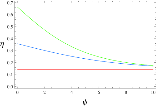
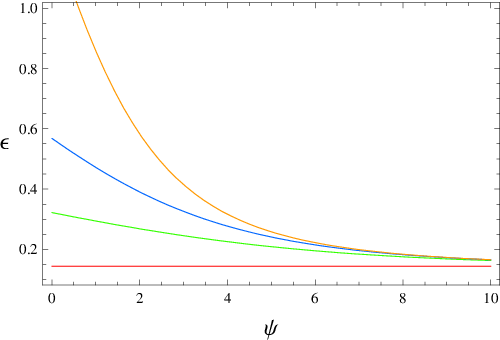
which reproduces the result of (33) in the appropriate limit. One notes that the value of decreases with increasing , for fixed . If one also increases , then one requires larger and larger values of in order to keep the parameter suppressed for inflation. Since inflation requires we see that this requires larger and larger as we increase the level of the interaction. To illustrate this we sketch the behaviour of the parameters as a function of for fixed in Figures 1 and 2. One notes that inflation must occur in the region where , and therefore as one includes higher order terms in , this condition becomes impossible to satisfy. Numerically we find the following lower bound on the number of branes
| (36) |
valid for , where is a constant of . The numerical coefficient is sensitive to the volume of the compact manifold. What is interesting to note is that the bound shifts by a constant factor as we increase the level of interaction. Since we are taking to be order unity, this implies is order unity, although the precise value also depends on the volume. For the canonical choices discussed previously, we find that and . The value of increases as we increase the volume, thus for we have whilst for we see that doubles to . If one refers back to the bound in (25) we see that the number of branes is bounded from above by causality arguments. Inflation will then only occur if the number of branes falls in between the relevant bound. For example we see that (setting )
| (37) |
Note that the latter bound cannot be satisfied for . Therefore eternal inflation will only occur precisely when and which is a highly tuned solution.
If one takes the potential at face value, then is appears that there is a large region of parameter space where inflation (although not of the simple power law kind) is possible, although eternal. Since we cannot parameterise the end of inflation in an obvious manner, the question of reheating is an important one. The issue is that the effective theory has a geometric origin when viewed from the UV, namely the fivebranes must eventually collide with the boundary branes. If the inflationary phase lasts this long, then one assumes that reheating will occur when the fivebranes merge with the boundary via instanton transitions. However this requires a more detailed understanding of the effective theory, since other terms in the superpotential must be included.
In the absence of such a procedure, one may ask if instant preheating may be used both as an end for inflation and also as a means to reheat the domain wall branes. A simple way in which this may be achieved is to consider an additional (effective) coupling between the inflaton and the volume modulus via [41, 42, 43]
| (38) |
where is related to the real part of the superfield through , is a bulk fermion field and represents the shifted inflaton such that inflation ends at . Since we cannot analytically control the end of inflation in these models, we should take it to represent the value of at which we expect other terms in the superpotential to become important.
VII Discussion
In this paper we have re-considered the power law inflation scenario proposed in the Heterotic M-theory model of [15] to better understand the regime of validity of the theory. As a consequence, we have determined the correct expression for the scalar potential in the presence of instanton interactions between the nearest neighbours and shown that this also leads to eternal inflation. By requiring the solution to be causal and have inflating trajectories we find the following numeric bound on the number of branes, valid for
| (39) |
where both and depend on the two volumes although for a large range of phenomenologically favoured parameters we expect . The dependence on the overall volume is the most sensitive, and we argued that for the volume , the above bound can only be satisfied when . This corroborates an intuitive result, namely that as we increase the number of interactions , the number of branes required to meet our inflationary requirement must also increase. This does not affect the solution [15], which corresponds to power law inflation, precisely because of the special nature of that model. More generally one can see that inflation with an arbitrary number of branes, and an arbitrary number of instanton interactions, is less likely. Whilst this is intuitive, it is worth investigating in some detail precisely because the Heterotic theory provides a very useful example where the standard model sector can be identified (in principle).
Our results also suggest that despite the beautiful simplicity of the assisted inflation scenario, there is a large drawback in that the theory breaks down once we begin to probe away from the region due to the assumption that the branes are localised near the centre of the orbifold. Whilst it is interesting to speculate on the small instanton transition which results in the branes dissolving into the boundary, one must bear in mind that the effective theory is no longer valid in this region, and one must include terms arising at the same order in the superpotential.
Acknowledgments
Thanks to Steve Thomas for his comments. JW is supported by EPSRC of Canada. PVM research was supported by the grant FEDER/POCI/FIS/P/57547/2004.
Appendix A Phase space
Since we have a canonical action, the equation of motion for the inflaton is given by the usual expression . If we define the following dimensionless variables
| (40) |
then we can define the following autonomous equations for the flow of these parameters via
| (41) | |||||
| (42) |
where primes denote derivatives with respect to and we will set at the end. The linearised perturbations about such a solution are therefore
| (43) | |||||
where the () ambiguity arises from taking the square root of the Hubble equation, and denotes a derivative with respect to and evaluated at . This is a matrix equation where for stability of the fixed points we require both eigenvalues to be negative (ie a positive determinant). To keep track of the ambiguity let us introduce and therefore the eigenvalues become
| (44) | |||||
where we have used and also
| (45) |
Clearly the stability depends on the choice of and also the scalar potential.
One can study the parametric flow of and as functions of time (assuming fixed and ), however the result is not illuminating enough to show. What we see is that the fixed points of the system are localised at and that increasing forces the trajectory lines to diverge from the point more and more rapidly. All the trajectories map onto one another as they approach the late time attractor point, as expected.
Let us consider the static solution for simplicity, since this is the only solution to . The other fixed point therefore occurs when , or when the potential is at an extremum. Since the potential is essentially runaway, this condition can only be satisfied for . In this instance the eigenvalue equation reduces to
| (46) |
and therefore we have the following solutions. For we find for stability and for we have . Ultimately however the phase space dynamics tell us that this fixed point solution occurs when has rolled down to the bottom of the potential. However this is beyond the regime of validity of the effective theory, since other terms in the inflaton potential will be non-vanishing in this regime.
References
- [1] P. Horava and E. Witten, Nucl. Phys. B 460, 506 (1996) [arXiv:hep-th/9510209].
- [2] P. Horava and E. Witten, Nucl. Phys. B 475, 94 (1996) [arXiv:hep-th/9603142].
- [3] D. Bailin, G. V. Kraniotis and A. Love, Phys. Lett. B 443, 111 (1998) [arXiv:hep-th/9808142].
- [4] A. Lukas, B. A. Ovrut and D. Waldram, JHEP 9904, 009 (1999) [arXiv:hep-th/9901017].
- [5] A. Lukas, B. A. Ovrut and D. Waldram, arXiv:hep-th/9812052.
- [6] J. Gray, A. Lukas and G. I. Probert, Phys. Rev. D 69, 126003 (2004) [arXiv:hep-th/0312111].
- [7] E. J. Copeland, J. Gray and A. Lukas, Phys. Rev. D 64, 126003 (2001) [arXiv:hep-th/0106285].
- [8] K. Becker, M. Becker, K. Dasgupta and P. S. Green, JHEP 0304, 007 (2003) [arXiv:hep-th/0301161].
- [9] G. Curio and A. Krause, Nucl. Phys. B 643, 131 (2002) [arXiv:hep-th/0108220].
- [10] E. I. Buchbinder and B. A. Ovrut, Phys. Rev. D 69, 086010 (2004) [arXiv:hep-th/0310112].
- [11] M. Becker, G. Curio and A. Krause, Nucl. Phys. B 693, 223 (2004) [arXiv:hep-th/0403027].
- [12] V. Braun, Y. H. He, B. A. Ovrut and T. Pantev, JHEP 0601, 025 (2006) [arXiv:hep-th/0509051].
- [13] E. I. Buchbinder, Nucl. Phys. B 711, 314 (2005) [arXiv:hep-th/0411062].
- [14] B. de Carlos, J. Roberts and Y. Schmohe, Phys. Rev. D 71, 026004 (2005) [arXiv:hep-th/0406171].
- [15] K. Becker, M. Becker and A. Krause, Nucl. Phys. B 715, 349 (2005) [arXiv:hep-th/0501130].
- [16] A. Krause, JCAP 0807, 001 (2008) [arXiv:0708.4414 [hep-th]].
- [17] J. Ward, Phys. Rev. D 73, 026004 (2006) [arXiv:hep-th/0511079].
- [18] A. Ashoorioon and A. Krause, arXiv:hep-th/0607001.
- [19] A. R. Liddle, A. Mazumdar and F. E. Schunck, Phys. Rev. D 58, 061301 (1998) [arXiv:astro-ph/9804177].
- [20] P. Kanti and K. A. Olive, Phys. Rev. D 60, 043502 (1999) [arXiv:hep-ph/9903524].
- [21] P. Kanti and K. A. Olive, Phys. Lett. B 464, 192 (1999) [arXiv:hep-ph/9906331].
- [22] E. J. Copeland, A. Mazumdar and N. J. Nunes, Phys. Rev. D 60, 083506 (1999) [arXiv:astro-ph/9904309].
- [23] T. Banks, M. Berkooz, S. H. Shenker, G. W. Moore and P. J. Steinhardt, Phys. Rev. D 52, 3548 (1995) [arXiv:hep-th/9503114].
- [24] P. Binetruy and M. K. Gaillard, Phys. Rev. D 34, 3069 (1986).
- [25] J. P. Conlon and F. Quevedo, JHEP 0601, 146 (2006) [arXiv:hep-th/0509012].
- [26] J. R. Bond, L. Kofman, S. Prokushkin and P. M. Vaudrevange, Phys. Rev. D 75, 123511 (2007) [arXiv:hep-th/0612197].
- [27] T. W. Grimm, Phys. Rev. D 77, 126007 (2008) [arXiv:0710.3883 [hep-th]].
- [28] R. Kallosh, N. Sivanandam and M. Soroush, Phys. Rev. D 77, 043501 (2008) [arXiv:0710.3429 [hep-th]].
- [29] A. Misra and P. Shukla, Nucl. Phys. B 800, 384 (2008) [arXiv:0712.1260 [hep-th]].
- [30] D. Battefeld, T. Battefeld and A. C. Davis, JCAP 0810, 032 (2008) [arXiv:0806.1953 [hep-th]].
- [31] D. Battefeld and T. Battefeld, JCAP 0903, 027 (2009) [arXiv:0812.0367 [hep-th]].
- [32] E. I. Buchbinder, Phys. Rev. D 70, 066008 (2004) [arXiv:hep-th/0406101].
- [33] J. P. Hsu, R. Kallosh and N. Sivanandam, JHEP 0601, 123 (2006) [arXiv:hep-th/0510254].
- [34] G. Curio and A. Krause, Phys. Rev. D 75, 126003 (2007) [arXiv:hep-th/0606243].
- [35] L. Anguelova and D. Vaman, Nucl. Phys. B 733, 132 (2006) [arXiv:hep-th/0506191].
- [36] L. Anguelova and K. Zoubos, Phys. Rev. D 74, 026005 (2006) [arXiv:hep-th/0602039].
- [37] J. Gray, A. Lukas and B. Ovrut, Phys. Rev. D 76, 066007 (2007) [arXiv:hep-th/0701025].
- [38] G. R. Dvali and S. H. H. Tye, Phys. Lett. B 450, 72 (1999) [arXiv:hep-ph/9812483].
- [39] M. Bastero-Gil, A. Berera, J. B. Dent and T. W. Kephart, arXiv:0904.2195 [astro-ph.CO].
- [40] L. Anguelova, V. Calo and M. Cicoli, arXiv:0904.0051 [hep-th].
- [41] G. N. Felder, L. Kofman and A. D. Linde, Phys. Rev. D 59, 123523 (1999) [arXiv:hep-ph/9812289].
- [42] G. N. Felder, L. Kofman and A. D. Linde, Phys. Rev. D 60, 103505 (1999) [arXiv:hep-ph/9903350].
- [43] S. Panda, M. Sami and I. Thongkool, arXiv:0905.2284 [hep-th].