Viscoelasticity is a notion that unifies solids and fluids (see [1] for example), and is applied to a wide range of materials as in rheology [2]. Viscoelastic materials behave as solids during short intervals of time, while they do as ordinary viscous fluids at long time scales [3, 4].

In order to get a concrete image for viscoelastic materials, let us imagine something like a chewing gum. We can see many particles bonding in it to each other (see Fig. 1). When the material is stressed, the bonds produce an elastic force and try to make the particles back to the original configuration. That is, the system exhibits elasticity during short intervals of time. However, if we keep the deformation for a long time, then the bonding structure changes to reduce the free energy as in Fig. 1, and the shear stress vanishes. We further assume that the material is elastic for compressions even for long time scales, so that the bulk stress does not undergo such relaxation (see Fig. 2). Thus the system exhibits fluidity at long intervals of time.

In this paper, we propose a framework in which the characteristics of elasticity and fluidity can be both dealt with on equal footings. We introduce two key ingredients. One is a new variable (to be called the intrinsic metric) which represents the bonding structures. The other is the gauge symmetry of foliation preserving diffeomorphisms (FPDs),¹¹ 1 An interesting application to quantum gravity was recently found by Ho$\check{\text{r}}$ava [5]. For mathematical details of FPDs, see also [6]. which we find to interpolate between the two extreme limits of elasticity and fluidity in a natural manner. We show that requiring the invariance under FPDs uniquely determines the dynamics of viscoelastic systems in the first order of strains.

For an elastic material, a sufficiently small region around any point can always be regarded as being deformed from the configuration with no strains. We call the shape before the deformation the natural shape (see Fig. 3). This is a straightforward generalization of the notion of the “natural length” for a spring or a rubber string. For a viscoelastic material, we assume that it exhibits the elasticity during short time intervals, so that we can define the natural shape around a given point at each moment. Since the natural shape is constant in time for elastic materials, its time dependence represents the plasticity (i.e. non-elasticity) of the material. In order to describe the natural shape quantitatively, we introduce a new dynamical variable to be called the intrinsic metric, and discuss its properties in this section.

At each time $t$, we introduce coordinates $\xi=(\xi^{a})$ $(a=1,2,3)$ arbitrarily on the material.²² 2 Here we assume that the coordinates $\xi$ move smoothly on the material as the time $t$ varies. We then define the intrinsic metric of the material (denoted by $g_{ab}(\xi,t)$) such that the distance between two points at $\xi$ and $\xi+d\xi$ at fixed time $t$ is given by the distance in the natural shape (see Fig. 4):

$\displaystyle ds^{2}=g_{ab}(\xi,t)\,d\xi^{a}d\xi^{b}\equiv\mbox{(length in the natural shape)}^{2}.$

(2.1)

We let $X^{i}(\xi,t)$ be the spatial Cartesian coordinates of the point with $\xi$ at $t$ . We emphasize that the intrinsic metric $g_{ab}(\xi,t)$ is independent of $X^{i}(\xi,t)$, and can differ from the induced metric,³³ 3 For a function $F(\xi,t)$ we write $\dot{F}=\partial F/\partial t$ and $\partial_{a}F=\partial F/\partial\xi^{a}$.

$\displaystyle h_{ab}(\xi,t)\equiv\partial_{a}X^{i}(\xi,t)\,\partial_{b}X^{i}(\xi,t)\,,$

(2.2)

which measures the distance in the real three-dimensional space (see Fig. 4). Note that their discrepancies

$\displaystyle\varepsilon_{ab}(\xi,t)\equiv\frac{1}{2}\,\bigl(h_{ab}(\xi,t)-g_{ab}(\xi,t)\bigr)$

(2.3)

represent the strain tensor of the system. In order to see this, let us consider an elastic material. We take the coordinates $\xi$ such that they move with the atoms and coincide with their Cartesian coordinates in the mechanical equilibrium. When the material is deformed slightly, the atom labeled with $\xi$ has the coordinates $X^{a}(\xi,t)=\xi^{a}+u^{a}(\xi,t)$, where $u^{a}(\xi,t)$ is the displacement vector, and we have

$\displaystyle h_{ab}=\delta_{ab}+\partial_{a}u_{b}+\partial_{b}u_{a}+\mathcal{O}(u^{2})\,.$

(2.4)

Since the intrinsic metric keeps taking the values in the mechanical equilibrium, $g_{ab}=\delta_{ab}$ , we have that $\varepsilon_{ab}=(1/2)(h_{ab}-g_{ab})\simeq(1/2)(\partial_{a}u_{b}+\partial_{b}u_{a})$. This shows that $\varepsilon_{ab}$ is certainly the strain tensor for elastic systems. In the following discussions, we make the linear approximation with respect to $\varepsilon_{ab}$ . This implies that for the quantities of $\mathcal{O}(\varepsilon_{ab})$ one can raise or lower vector indices by either of $g_{ab}$ or $h_{ab}$ .

We denote by $\rho_{0}$ the mass density in the absence of strains. In this paper, we assume that $\rho_{0}$ is a constant independent of $\xi$ and $t$. Then the mass contained in a volume element $d^{3}\xi=d\xi^{1}d\xi^{2}d\xi^{3}$ is given by $\rho_{0}\sqrt{g(\xi,t)}\,d^{3}\xi$, and the mass density in the real three-dimensional space is given by

$\displaystyle\rho(\xi,t)=\frac{\rho_{0}\sqrt{g(\xi,t)}\,d^{3}\xi}{\sqrt{h(\xi,t)}\,d^{3}\xi}=\frac{\sqrt{g(\xi,t)}}{\sqrt{h(\xi,t)}}\,\rho_{0}\,.$

(2.5)

As an example, let us consider a squeeze deformation of a two-dimensional viscoelastic material formed by bonding particles as in Fig. 5 .

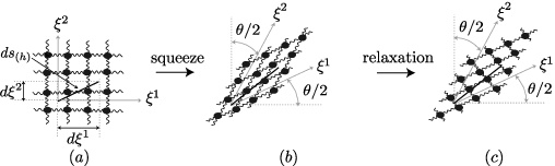
The wavy lines stand for the bonds. The left figure represents the material before the deformation. Here we take $\xi$ to be Cartesian coordinates, and then both of the induced and intrinsic metrics have the same form: $h_{ab}=g_{ab}=\delta_{ab}$ . Therefore the mass density $\rho$ is equal to $\rho_{0}$ . We assume that $\xi$ are attached to the particles, so that they comove with the material under the deformation. The middle figure represents the material just after the deformation. The induced metric and the mass density change according to the deformation, while the intrinsic metric does not. The induced metric is evaluated as $ds^{2}=(d\xi^{1})^{2}+(d\xi^{2})^{2}-2d\xi^{1}d\xi^{2}\cos(\pi/2+\theta)$  by using the cosine formula. The right figure represents the material after a sufficiently long time. In the process of relaxation, the induced metric and the mass density are preserved, while the intrinsic metric $g_{ab}$ becomes proportional to $h_{ab}$ ,  $g_{ab}=f(\xi,t)\,h_{ab}$ , as will be discussed around (4.7) . The factor $f(\xi,t)$ can be determined from $\rho$ through (2.5).

Since we have introduced a different coordinate system $\xi$ at each time, in order to describe the actual motion of a material one needs to specify how the fluid particles move relatively to the coordinate system $\xi$. This can be realized by introducing a vector field $N^{a}(\xi,t)$, with which the fluid particle located at $\xi$ at time $t$ is supposed to move to the position $\xi^{a}+N^{a}(\xi,t)\delta t$ after the time interval $\delta t$ (see Fig. 6).

In fact, by using $N^{a}$, the time derivative along the path of a fluid particle (the material derivative) of a scalar quantity $\varphi(\xi,t)$ can be expressed as

$\displaystyle\frac{D\varphi}{Dt}=\dot{\varphi}+N^{a}\partial_{a}\varphi\,.$

(3.1)

For example, when measured in the real space, the velocity $v^{i}(\xi,t)$ and the acceleration $a^{i}(\xi,t)$ of the fluid particle located at $\xi$ are given by

	$\displaystyle v^{i}$	$\displaystyle=\frac{DX^{i}}{Dt}=\dot{X}^{i}+N^{a}\partial_{a}X^{i},$		(3.2)
	$\displaystyle a^{i}$	$\displaystyle=\frac{Dv^{i}}{Dt}=\dot{v}^{i}+N^{a}\partial_{a}v^{i}.$		(3.3)

Then we consider the foliation preserving diffeomorphism (FPD):

$\displaystyle t^{\prime}=t,\qquad\xi^{\prime}{}^{a}=\xi^{\prime}{}^{a}(\xi,t).$

(3.4)

We say that a quantity $T^{a\cdots}_{~~~b\cdots}(\xi,t)$ is a covariant tensor, if it transforms as a three-dimensional tensor at each time:

$\displaystyle T^{\prime}\,{}^{a\cdots}_{~~~b\cdots}(\xi^{\prime},t)=\frac{\partial\xi^{\prime}{}^{a}}{\partial\xi^{c}}\cdots\frac{\partial\xi^{d}}{\partial\xi^{\prime}{}^{b}}\cdots T^{c\cdots}_{~~~d\cdots}(\xi,t)\,,$

(3.5)

where the transition functions $\partial\xi^{\prime}{}^{a}/\partial\xi^{c}$ and $\partial\xi^{d}/\partial\xi^{\prime}{}^{b}$ should be evaluated at time $t$. For example, $X^{i}$, $v^{i}$ and $a^{i}$ are covariant scalars, and $g_{ab}$, $h_{ab}$ and $\varepsilon_{ab}$ are rank two covariant tensors.

On the other hand, $N^{a}$ is not a covariant vector but transforms with an inhomogeneous term:⁴⁴ 4 This is naturally understood, if one recognizes that $N^{a}$ can be regarded as a gauge field that appears when the three-dimensional diffeomorphism is gauged in the time direction.

$\displaystyle N^{\prime}{}^{a}(\xi^{\prime},t)=\frac{\partial\xi^{\prime}{}^{a}(\xi,t)}{\partial\xi^{b}}N^{b}(\xi,t)+\frac{\partial\xi^{\prime}{}^{a}(\xi,t)}{\partial t}\,.$

(3.6)

To see this, let us consider a fluid particle in two different coordinate systems, and assume that it has the coordinates $\xi^{a}$ and $\xi^{\prime}{}^{a}$, respectively, at time $t$. Then, by definition, at time $t+\delta t$, they become $\xi^{a}+N(\xi,t)\delta t$ and $\xi^{\prime}{}^{a}+N^{\prime}{}^{a}(\xi^{\prime},t)\delta t$, respectively. Because these are related by the transformation (3.4) at $t+\delta t$, we have

	$\displaystyle\xi^{\prime}{}^{a}+N^{\prime}{}^{a}(\xi^{\prime},t)\delta t$	$\displaystyle=\xi^{\prime}{{}^{a}}(\xi+N(\xi,t)\delta t,\,t+\delta t)$
		$\displaystyle=\xi^{\prime}{}^{a}+\frac{\partial\xi^{\prime}{}^{a}(\xi,t)}{\partial\xi^{b}}N^{b}(\xi,t)\delta t+\frac{\partial\xi^{\prime}{}^{a}(\xi,t)}{\partial t}\delta t,$		(3.7)

and thus we obtain (3.6).

Note that the time derivative of a covariant tensor $T^{a\cdots}_{~~~b\cdots}$ is no longer covariant. We, however, can make a covariant tensor by considering the derivative along fluid particles as in (3.2) and (3.3):

$\displaystyle\frac{D}{Dt}\,T^{a\cdots}_{~~~b\cdots}=\dot{T}^{a\cdots}_{~~~b\cdots}+{\mathcal{L}}_{\mathcal{N}}\,T^{a\cdots}_{~~~b\cdots}\,,$

(3.8)

where ${\mathcal{L}}_{\mathcal{N}}$ is the Lie derivative with respect to the vector field ${\mathcal{N}}=N^{a}\partial_{a}$ :

$\displaystyle{\cal L}_{\mathcal{N}}\,T^{a\cdots}_{~~~b\cdots}=N^{c}\partial_{c}T^{a\cdots}_{~~~b\cdots}-\partial_{c}N^{a}T^{c\cdots}_{~~~b\cdots}-\cdots+\partial_{b}N^{c}T^{a\cdots}_{~~~c\cdots}+\cdots.$

(3.9)

For example, from $g_{ab}$, we can make a covariant tensor $K_{ab}$ to be called the extrinsic curvature,

$\displaystyle K_{ab}=\frac{1}{2}\,\frac{Dg_{ab}}{Dt}=\frac{1}{2}\,\bigl(\dot{g}_{ab}+\partial_{a}N^{c}\,g_{cb}+\partial_{b}N^{c}\,g_{ac}+N^{c}\,\partial_{c}g_{ab}\bigr).$

(3.10)

Similarly, we can define the extrinsic curvature $K_{ab}^{(h)}$ which corresponds to $h_{ab}$,

$\displaystyle K_{ab}^{(h)}=\frac{1}{2}\,\frac{Dh_{ab}}{Dt}=\frac{1}{2}\,\bigl(\dot{h}_{ab}+\partial_{a}N^{c}\,h_{cb}+\partial_{b}N^{c}\,h_{ac}+N^{c}\,\partial_{c}h_{ab}\bigr).$

(3.11)

Note that

$\displaystyle K_{ab}^{(h)}-K_{ab}=\frac{D\varepsilon_{ab}}{Dt}\,.$

(3.12)

We then introduce the dreibeins $e^{i}_{a}(\xi,t)$ and their inverses $e^{a}_{i}(\xi,t)$ :

$\displaystyle e^{i}_{a}(\xi,t)=\partial_{a}X^{i}(\xi,t)\,,\qquad e^{a}_{i}\,e^{i}_{b}=\delta^{a}_{b}\,.$

(3.13)

From (3.2) and (3.13), we obtain

$\displaystyle h_{ab}=e_{a}^{i}e_{b}^{i}\,,\qquad\partial_{a}e_{b}^{i}=\partial_{b}e_{a}^{i}\,,\qquad\dot{e}_{a}^{i}=\partial_{a}v^{i}-(\partial_{a}N^{b})e^{i}_{b}-N^{b}\partial_{a}e_{b}^{i}\,,$

(3.14)

and thus

$\displaystyle\frac{De_{a}^{i}}{Dt}=\partial_{a}v^{i}.$

(3.15)

By using the dreibeins, the scalars $v^{i}(\xi,t)$ and $a^{i}(\xi,t)$ can be transformed into vector fields as

$\displaystyle v^{a}$

$\displaystyle\equiv e^{a}_{i}v^{i},\qquad v_{a}\equiv e_{a}^{i}v^{i},\qquad a^{a}\equiv e^{a}_{i}a^{i},\qquad a_{a}\equiv e_{a}^{i}a^{i}.$

(3.16)

We can calculate the acceleration $a_{a}$ by using the Leibniz rule for $D/Dt$ and (3.15) as

	$\displaystyle a_{a}$	$\displaystyle=e_{a}^{i}\frac{Dv^{i}}{Dt}=\frac{D(e_{a}^{i}v^{i})}{Dt}-v^{i}\frac{De_{a}^{i}}{Dt}=\frac{Dv_{a}}{Dt}-\partial_{a}\left(\frac{1}{2}(v^{i})^{2}\right)$
		$\displaystyle=\dot{v}_{a}+(\partial_{a}N^{b})v_{b}+N^{b}\partial_{b}v_{a}-\partial_{a}\left(\frac{1}{2}v^{b}v_{b}\right).$		(3.17)

Furthermore, by using the first of (3.14) and (3.15), we can show

$\displaystyle K_{ab}^{(h)}=\frac{1}{2}\left((\partial_{a}v^{i})\,e_{b}^{i}+(\partial_{b}v^{i})\,e_{a}^{i}\right)=\frac{1}{2}\left(\nabla_{a}^{(h)}v_{b}+\nabla_{b}^{(h)}v_{a}\right).$

(3.18)

The set of FPDs forms a gauge symmetry group of the system, which can be gauge-fixed arbitrarily according to convenience in describing the dynamics of a given system. Two of the useful gauge fixings are the followings:

We are now in a position to write down a set of equations which determine the time evolution of $X^{i}(\xi,t)$, $g_{ab}(\xi,t)$ and $N^{a}(\xi,t)$ up to FPDs. The covariance under FPDs is found to be powerful enough to uniquely determine the dynamics in the first order of $\varepsilon_{ab}$ .

We first consider the limiting case of elasticity. Due to our definition of the intrinsic metric, $g_{ab}(\xi,t)$ should be constant in time for elastic materials in the comoving frame ($N^{a}=0$). The FPD-covariant expression for this statement is that the extrinsic curvature $K_{ab}$ of (3.10) vanishes:

$\displaystyle K_{ab}=0\quad\mbox{(elastic limit)}\,.$

(4.1)

This implies that the non-vanishing $K_{ab}$ represents the genuinely plastic deformations.

In order to make further discussions, we need to separate the trace part from $K_{ab}$ because it vanishes for any materials due to the mass conservation of the system:

$\displaystyle K(\xi,t)\equiv g^{ab}(\xi,t)K_{ab}(\xi,t)=0\,.$

(4.2)

In fact, contracting (3.10) with $g^{ab}$, we obtain

	$\displaystyle K$	$\displaystyle=\frac{1}{2}\,g^{ab}\bigl(\dot{g}_{ab}+\partial_{a}N^{c}\,g_{cb}+\partial_{b}N^{c}\,g_{ac}+N^{c}\,\partial_{c}g_{ab}\bigr)$
		$\displaystyle=\frac{1}{\sqrt{g}}\,\bigl((\sqrt{g}\,)^{\mbox{{$\cdot$}}}+\partial_{a}(\sqrt{g}N^{a})\bigr)$
		$\displaystyle=\frac{1}{\rho_{\text{int}}}\,\bigl(\dot{\rho}_{\text{int}}+\partial_{a}(\rho_{\text{int}}N^{a})\bigr),$		(4.3)

where $\rho_{\text{int}}(\xi,t)=\rho_{0}\sqrt{g(\xi,t)}$ is the mass density with respect to the intrinsic metric. This indicates that the vanishing of $K$ is equivalent to the mass conservation, which can be easily seen in the comoving frame where $N^{a}=0$ and $\dot{\rho}_{\text{int}}=0$.

The traceless part of $K_{ab}$ on the other hand describes the rate of the shear deformation of the intrinsic metric, and thus is expected to be proportional to the traceless part of the strain tensor

$\displaystyle\tilde{K}_{ab}(\xi,t)=\frac{1}{\tau}\,\tilde{\varepsilon}_{ab}(\xi,t)\,,$

(4.4)

where $\tau$ is the relaxation time, and

	$\displaystyle\tilde{K}_{ab}$	$\displaystyle\equiv K_{ab}-\frac{1}{3}Kg_{ab}\,,$		(4.5)
	$\displaystyle\tilde{\varepsilon}_{ab}$	$\displaystyle\equiv\varepsilon_{ab}-\frac{1}{3}\,(g^{cd}\varepsilon_{cd})\,g_{ab}\,.$		(4.6)

We call (4.4) the rheology equation hereafter. After a time interval much longer than $\tau$, $\tilde{\varepsilon}_{ab}(\xi,t)$ vanishes and thus $g_{ab}(\xi,t)$ becomes proportional to $h_{ab}(\xi,t)$:

$\displaystyle g_{ab}(\xi,t)=f(\xi,t)\,h_{ab}(\xi,t)\quad\quad(f(\xi,t):\text{a scalar function})\,,$

(4.7)

where $f(\xi,t)$ is determined by the mass conservation as in the example in Sec. 2.

The equation (4.4) is the simplest and is expected to be universal. It is consistent with (4.1) because the elastic limit corresponds to $\tau=\infty$ . The fluid limit is also realized correctly by taking $\tau=0$ , in which we have $\tilde{\varepsilon}_{ab}=0$ . This implies that $g_{ab}$ is proportional to $h_{ab}$ as in (4.7). The only remaining degree of freedom of $g_{ab}$ becomes the density of the material, which means that the system corresponds to an isotropic fluid.

Note that (4.2) and (4.4) indicate that all the components of $K_{ab}$ are of the order $\varepsilon$. Then from (3.12) we find that so are those of $K^{(h)}_{ab}$, and we have

		$\displaystyle\tilde{K}_{ab}^{(h)}-\tilde{K}_{ab}=\frac{D\tilde{\varepsilon}_{ab}^{(h)}}{Dt}+\mathcal{O}(\varepsilon^{2})\,,$		(4.8)
		$\displaystyle K^{(h)}-K=\frac{D\varepsilon^{(h)}}{Dt}+\mathcal{O}(\varepsilon^{2})\,.$		(4.9)

The dynamics of $X^{i}(\xi,t)$ should be expressed as Euler’s equation which is written with the stress tensor $T_{ab}$ as

$\displaystyle\rho\,a_{a}=-\nabla^{(h)b}T_{ba}\,,$

(4.10)

where $\nabla^{(h)}$ is the covariant derivative with respect to $h_{ab}$ . We show that the leading form of the stress tensor in the derivative expansion can be determined by the following requirements:

• •

  $T_{ab}$ is symmetric and covariant under FPDs.

• •

  $T_{ab}$ is linear in the strain $\varepsilon_{ab}$ and the spatial derivative of the velocity, $\nabla_{a}^{(h)}v_{b}$.

The above requirements imply that $T_{ab}$ is a linear combination of the irreducible components of $\varepsilon_{ab}$ and $K_{ab}^{(h)}=(1/2)(\nabla_{a}^{(h)}v_{b}+\nabla_{b}^{(h)}v_{a})$ (see (3.18)):

$\displaystyle T_{ab}=-2\mu\,\tilde{\varepsilon}_{ab}^{(h)}-\frac{1}{\kappa}\,\varepsilon^{(h)}\,h_{ab}-2\gamma\,\tilde{K}_{ab}^{(h)}-\zeta\,K^{(h)}h_{ab}\,,$

(4.11)

where

	$\displaystyle\varepsilon^{(h)}$	$\displaystyle\equiv h^{ab}\varepsilon_{ab}\,,$		(4.12)
	$\displaystyle\tilde{\varepsilon}_{ab}^{(h)}$	$\displaystyle\equiv\varepsilon_{ab}-\frac{1}{3}\varepsilon^{(h)}h_{ab}\,,$		(4.13)
	$\displaystyle K^{(h)}$	$\displaystyle\equiv h^{ab}K_{ab}^{(h)}\,,$		(4.14)
	$\displaystyle\tilde{K}_{ab}^{(h)}$	$\displaystyle\equiv K_{ab}^{(h)}-\frac{1}{3}K^{(h)}h_{ab}\,.$		(4.15)

From the discussions around (4.8), we find that all the terms in (4.11) are of the order of $\varepsilon$.

In order to see the meaning of the coefficients in (4.11), we consider two extreme limits of elasticity and fluidity. We first consider the elastic limit. Since $K_{ab}=0$ in the elastic limit (see (4.1)), the formulas (4.8) and (4.9) lead to

	$\displaystyle\tilde{K}_{ab}^{(h)}=\frac{D\tilde{\varepsilon}_{ab}^{(h)}}{Dt}\left(1+\mathcal{O}(\varepsilon)\right),$		(4.16)
	$\displaystyle K=\frac{D\varepsilon^{(h)}}{Dt}\left(1+\mathcal{O}(\varepsilon)\right),$		(4.17)

and thus we have

$\displaystyle T_{ab}\simeq-2\,\mu\,\tilde{\varepsilon}_{ab}^{(h)}-\frac{1}{\kappa}\,\varepsilon^{(h)}h_{ab}-2\gamma\frac{D\tilde{\varepsilon}_{ab}^{(h)}}{Dt}-\zeta\frac{D\varepsilon^{(h)}}{Dt}h_{ab}\quad(\mbox{elastic limit})\,.$

(4.18)

This indicates that the parameters $\mu$ and $1/\kappa$ are the shear and bulk moduli, respectively. The last two terms express frictions.

On the other hand, the fluid limit is realized by considering the case where the time scale $T$ of the variation of the shear strain $\tilde{\varepsilon}_{ab}$,

$\displaystyle\frac{D}{Dt}\,\tilde{\varepsilon}_{ab}\sim\frac{1}{T}\,\tilde{\varepsilon}_{ab}\,,$

(4.19)

is much longer than the relaxation time $\tau$, $T\gg\tau$. We then can show that

$\displaystyle\tilde{K}_{ab}=\tilde{K}_{ab}^{(h)}\left(1+\mathcal{O}\left(\frac{\tau}{T}\right)\right)\,,$

(4.20)

because the following holds due to (4.8):

$\displaystyle\tilde{K}_{ab}^{(h)}-\tilde{K}_{ab}=\frac{D\tilde{\varepsilon}_{ab}^{(h)}}{Dt}\left(1+\mathcal{O}(\varepsilon)\right)=\frac{D\tilde{\varepsilon}_{ab}}{Dt}\left(1+\mathcal{O}(\varepsilon)\right)\sim\frac{1}{T}\,\tilde{\varepsilon}_{ab}=\frac{\tau}{T}\tilde{K}_{ab}\,.$

(4.21)

Since $\tilde{\varepsilon}^{(h)}_{ab}=\tilde{\varepsilon}_{ab}\left(1+\mathcal{O}(\varepsilon)\right)=\tau\,\tilde{K}_{ab}\,\bigl(1+\mathcal{O}(\varepsilon)\bigr)$, we can rewrite the stress tensor (4.11) into

$\displaystyle T_{ab}\simeq-2\eta\,\tilde{K}_{ab}^{(h)}-\zeta\,K^{(h)}h_{ab}-\frac{1}{\kappa}\,\varepsilon^{(h)}\,h_{ab}\quad(\mbox{fluid~limit})\,,$

(4.22)

where

$\displaystyle\eta\equiv\gamma+\mu\,\tau\,.$

(4.23)

By using (3.18), each term in (4.22) can be interpreted in terms of fluid mechanics if we take the laboratory frame ($X^{a}(\xi,t)=\xi^{a}$, $v^{a}=N^{a}$):

	$\displaystyle h_{ab}$	$\displaystyle=\delta_{ab}\,,$		(4.24)
	$\displaystyle\tilde{K}^{(h)}_{ab}$	$\displaystyle=\frac{1}{2}\,(\partial_{a}v_{b}+\partial_{b}v_{a})-\frac{1}{3}\,\partial_{c}v_{c}\,\delta_{ab}\,,$		(4.25)
	$\displaystyle K^{(h)}$	$\displaystyle=h^{ab}K^{(h)}_{ab}=\partial_{c}v_{c}\,,$		(4.26)

which indicates that $\eta$ and $\zeta$ represent the shear and bulk viscosities of the fluid, respectively.⁵⁵ 5 The equation (4.23) shows that the shear viscosity consists of two contributions. The first term $\gamma$ reflects the friction which the material already has in the elastic limit, while the second term $\mu\tau$ represents the stress caused by the strain as the material undergoes plastic deformations [4]. The third term in (4.22) can be interpreted as the pressure:

$\displaystyle p=-\frac{1}{\kappa}\,\varepsilon^{(h)}\,.$

(4.27)

To see this, we notice that $\varepsilon^{(h)}$ ($\simeq(\sqrt{h}-\sqrt{g}\,)/\sqrt{g}$ ) measures the deviation of the real volume element from that of the natural shape,⁶⁶ 6 Note that in the linear order of $\varepsilon_{ab}^{(h)}$ we have $\displaystyle\frac{\sqrt{h}-\sqrt{g}}{\sqrt{g}}=\frac{\sqrt{\det(g_{ab}+2\,\varepsilon_{ab}^{(h)})}-\sqrt{g}}{\sqrt{g}}\simeq\varepsilon^{(h)}.$ and that the pressure vanishes in the natural shape. Therefore $p$ must be proportional to $-\varepsilon^{(h)}$. We then find that $\kappa$ agrees with the coefficient of compression because $\kappa=\rho\,d\rho^{-1}/dp\bigr|_{\rho=\rho_{0}}$ ($\rho=\rho_{0}\sqrt{g}\simeq\rho_{0}(1-\varepsilon^{(h)})$ and $p=-\kappa^{-1}\varepsilon^{(h)}$).

The set of equations (4.2), (4.4), (4.10), (4.11) and (4.23) are the fundamental equations which govern the dynamics of a given viscoelastic material. We can see that macroscopic properties of such materials are characterized only by six parameters $(\rho_{0},\,\tau,\,\eta,\,\zeta,\,\kappa,\gamma)$ from which another parameter $\mu$ is obtained via (4.23).

We have proposed a set of fundamental equations to describe generic viscoelastic systems in a unified way. It is expressed as a world volume theory with the target space coordinates $X^{i}(\xi,t)$ and the intrinsic metric $g_{ab}(\xi,t)$. FPDs play an important role in interpolating the two extreme limits of elasticity and fluidity. We have shown that the covariance under FPDs uniquely determines the form of the equations in the first order of strains. We thus conclude that the set of equations gives a universal description of viscoelastic systems.

Here we have considered viscoelastic systems with a single relaxation time. It would be interesting to consider a generalization to the case with more than one relaxation time in order to describe more realistic materials realized in laboratories.

This work was supported by the Grant-in-Aid for the Global COE program “The Next Generation of Physics, Spun from Universality and Emergence” from the Ministry of Education, Culture, Sports, Science and Technology (MEXT) of Japan. TA is also supported by the Japan Society for the Promotion of Science (JSPS) for Young Scientists (No. 20$\cdot$892). MF and HK are also supported by the Grant-in-Aid for Scientific Research No. 19540288 and No. 18540264, respectively, from MEXT.

References

- [1] R. M. Christensen, “Theory of Viscoelasticity,” Academic Press (1971).
- [2] E. C. Bingham, “Fluidity and Plasticity,” McGraw-Hill (1922).
- [3] L. D. Landau and E. M. Lifshitz, “Fluid Mechanics,” Butterworth-Heinemann, second edition (1987).
- [4] L. D. Landau and E. M. Lifshitz, “Theory of Elasticity,” Butterworth-Heinemann, third edition (1986).
- [5]
P. Hoava,
“Membranes at Quantum Criticality,”
JHEP 0903 (2009) 020 [arXiv:0812.4287 [hep-th]].
P. Hoava, “Quantum Gravity at a Lifshitz Point,” Phys. Rev. D 79 (2009) 084008 [arXiv:0901.3775 [hep-th]]. - [6]
H. B. Lawson Jr.,
“Foliations,”
Bull. Amer. Math. Soc. 80 (1974) 369.
C. Godbillon, “ Foeuilletages,” Birkhuser (1991).
I. Moerdijk and J. Mrum, “Introduction to Foliations and Lie Groupoids,” Cambridge University Press (2003).