Instability of Small Lovelock Black Holes in Even-dimensions

It is well known that string theory can be formulated only in ten dimensions. Hence, it is necessary to reconcile this prediction with our real world by compactifying extra-dimensions or by considering braneworld. Intriguingly, in the context of the braneworld with large extra-dimensions, black holes could be created at the TeV scale [1]. Hence, the stability of higher dimensional black holes becomes important since these black holes could be produced at the LHC if the spacetime has larger than six dimensions.

The stability of higher dimensional black holes has been an active topic since the seminal papers by Kodama and Ishibashi [2]. It is important to study various black holes in Einstein theory because black holes produced at the LHC are expected to be charged or rotating. A numerical study of charged black holes has been done [3]. To investigate the stability of rotating black holes, a group theoretical method is developed [4]. The method is used to study the stability of squashed black holes [5, 6] and 5-dimensional rotating black holes [7]. The stability of rotating black holes in more than 5-dimensions is also studied [8, 9, 10]. It is also important to consider the stability of black holes in more general gravitational theories because black holes are produced at the Planck scale where Einstein theory would be no longer valid. In fact, it is known that Einstein theory is merely a low energy limit of string theory [11]. In string theory, there are higher curvature corrections in addition to Einstein-Hilbert term [11]. Thus, it is natural to extend gravitational theory into those with higher power of curvature in higher dimensions. It is Lovelock theory that belongs to such class of theories [12]. In Lovelock theory, it is known that there exist static black hole solutions [13]. Hence, it is natural to suppose black holes produced at the LHC are of this type [14]. Thus, it is important to study the stability of these Lovelock black holes.

In the case of second order Lovelock theory, the so-called Einstein-Gauss-Bonnet theory, the stability analysis under tensor perturbations has been performed [15] (see also an earlier work [16]). The analysis has been also extended to the scalar and vector perturbations [17]. It is shown that there exists the scalar mode instability in five dimensions, the tensor mode instability in six dimensions, and no instability in other dimensions. In the case of third order Lovelock theory, the stability analysis of Lovelock black holes under tensor perturbations has been done by us [18]. We have shown that there is the instability for small black holes in eight dimensions. Although third order Lovelock theory is the most general theory in seven and eight dimensions, it is not so in more than eight dimensions. For example, when we consider ten dimensional black holes, we need to incorporate fourth order Lovelock terms. Indeed, when we consider black holes at the LHC, it is important to consider these higher order Lovelock terms [19]. Hence, in this paper, we study the stability of black holes in any order Lovelock theory, namely, in any dimensions.

The organization of this paper is as follows. In Section II, we review Lovelock theory and explain a graphical method for constructing Lovelock black hole solutions. In Section III, we present a master equation for tensor perturbations in the background of Lovelock black holes and reveal its universal structure. In Section IV, we examine the stability of Lovelock black holes with the method developed previously [18]. Finally, we summarize our results in Section V.

In this section, we review Lovelock theory and introduce a graphical method to obtain asymptotically flat black hole solutions.

In [12], the most general symmetric, divergence free rank (1,1) tensor is constructed out of a metric and its first and second derivatives. The corresponding Lagrangian can be constructed from $m$-th order Lovelock terms

where $R_{\lambda\sigma}{}^{\rho\kappa}$ is the Riemann tensor in $D$-dimensions and $\delta^{\lambda_{1}\sigma_{1}\cdots\lambda_{m}\sigma_{m}}_{\rho_{1}\kappa_{1}\cdots\rho_{m}\kappa_{m}}$ is the generalized totally antisymmetric Kronecker delta. Then, Lovelock Lagrangian in $D$-dimensions is defined by

where we define the maximum order $k\equiv[(D-1)/2]$ and $c_{m}$ are arbitrary constants. Here, $[z]$ represents the maximum integer satisfying $[z]\leq z$. Hereafter, we set $c_{0}=-2\Lambda$, $c_{1}=1$ and $c_{m}=a_{m}/m\ (m\geq 2)$ for convenience. Taking variation of the Lagrangian with respect to the metric, we can derive Lovelock equation

As is shown in [13], there exist static exact solutions of Lovelock equation. Let us consider the following metric

where ${\bar{\gamma}}_{ij}$ is the metric of $n\equiv D-2$-dimensional constant curvature space with a curvature $\kappa$=1,0 or -1. Using this metric ansatz, we can calculate Riemann tensor components as

Substituting (5) into (3) and defining a new variable $\psi(r)$ by

we obtain an algebraic equation

In (7), we used $n=D-2$ and $\mu$ is a constant of integration which is related to the ADM mass as [20]:

where we used a unit $16\pi G=1$.

From (7), it is easy to see that $f(r)$ has many branches. In this paper, we want to concentrate on asymptotically flat spherically symmetric, $\kappa=1$, solutions with a positive ADM mass $\mu>0$ because such black holes could be created at the LHC. We also assume that Lovelock coefficients satisfy

for simplicity. For example, consider $n=5$ for which Eq.(7) becomes third order algebraic equation. Though we have a formula for solutions of Eq.(7) in this case, the roots are too complicated in general. Hence, we use a graphical method illustrated in Fig.1. Because of the conditions (9), the function is monotonic for positive $\psi$. From (7), we see the root behaves $\psi\sim\mu/r^{n+1}$ or $f(r)\sim 1-\mu/r^{n-1}$ as $r\rightarrow\infty$. Thus, the asymptotically flat solutions belong to the branch where $\psi$ is always positive.

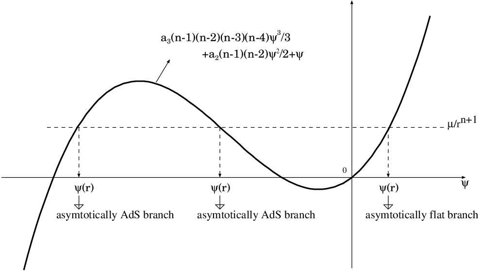
Note that the horizon radius of the asymptotically flat solution is characterized by $f(r_{H})=0$. From (6), we have a relation $\psi_{H}\equiv\psi(r_{H})=1/r_{H}^{2}$. Using this relation and (7), we obtain an algebraic equation

This determines $\psi_{H}$ and hence $r_{H}$. In Fig.2, we present a graphical method to solve Eq.(10). It is obvious from Fig.2 that $\infty\geq r\geq r_{H}$ corresponds to $0\leq\psi\leq\psi_{H}$ when $f(r)$ describes an asymptotically flat solution. It is also obvious that $\psi_{H}$ becomes larger as $\mu$ is smaller. Note that there may be no horizon if $\mu$ is too small (for example, in seven dimensions, there is no horizon if $0\leq\mu\leq 8a_{3}-9a_{2}^{2}$).

Using the metric ansatz (4), the Kretschmann scalar $R_{abcd}R^{abcd}$ is

Then, this solution has curvature singularities at $r=0$ or where derivatives of $f(r)$ diverges. For asymptotically flat spherical symmetric solutions, the conditions $|1-f|<\infty$, $|f^{{}^{\prime}}|<\infty$ and $|f^{{}^{\prime\prime}}|<\infty$ are satisfied except for $r=0$. Therefore, there is a curvature singularity only at $r=0$ in the cases we are considering. And asymptotically flat solutions have a horizon if the parameter $\mu$ is sufficiently large. So, this solution doesn’t have a naked singularity and describes a black hole with a mass M defined in (8) and no angular momentum.

To analyze the stability, it is convenient to decompose the metric under the symmetry of $n$-dimensional symmetric space. There are scalar, vector, and tensor modes. In this paper, we study tensor perturbations. In this section, we do not restrict parameters.

We consider tensor perturbations around the solution (4)

where $a,b=(t,r)$ and $\phi(t,r)$ represents the dynamical degrees of freedom. Here, $\bar{h}_{ij}$ are defined by

Here, $\bar{\nabla}^{i}$ denotes a covariant derivative with respect to $\bar{\gamma}_{ij}$. Here, the eigenvalue is given by $\gamma=-\ell(\ell+n-1)+2$, ($\ell=2,3,4\cdots$) for $\kappa=1$ and negative real number for $\kappa=-1,0$.

Perturbing the Lovelock equation (3), we can get the first order perturbation equation

where $\delta R_{ab}{}^{cd}$ represents the first order variation of the Riemann tensor. Since we are considering tensor perturbations, apparently we have $\delta{\cal G}_{a}{}^{b}=\delta{\cal G}_{a}{}^{i}=0$. To calculate $\delta{\cal G}_{i}^{j}$, we only need $\delta R_{ti}{}^{tj}$, $\delta R_{ri}{}^{rj}$ and $\delta R_{ij}{}^{kl}$. The reason is simple. We consider, for example, the term proportional to $\delta R_{tk}{}^{lm}$ in $\delta{\cal G}_{i}{}^{j}$. This means $\lambda_{m}=t$ or $\sigma_{m}=t$ in (13); and $\rho_{m}\neq t$ and $\kappa_{m}\neq t$. Since $\delta_{\rho_{1}\kappa_{1}\cdots}^{\lambda_{1}\sigma_{1}\cdots}$ consists of Kronecker delta, there must exist $\ell\ (1\leq\ell\leq m-1)$ such that $\rho_{\ell}=t$ or $\kappa_{\ell}=t$. Then $\lambda_{\ell}$ or $\sigma_{\ell}$ must be $t$ because of background Riemann tensor (5). So, for example, $\lambda_{m}$ and $\lambda_{\ell}$ become $t$. Noticing that $\delta_{\rho_{1}\kappa_{1}\cdots}^{\lambda_{1}\sigma_{1}\cdots}$ is totally antisymmetric, we see $\delta_{\rho_{1}\kappa_{1}\cdots}^{\lambda_{1}\sigma_{1}\cdots}=0$ when $\lambda_{m}=\lambda_{\ell}$. Thus, the coefficient of $\delta R_{tk}{}^{lm}$ in $\delta{\cal G}_{i}{}^{j}$ must be 0. For the same reason, coefficients of other than $\delta R_{ti}{}^{tj}$, $\delta R_{ri}{}^{rj}$ and $\delta R_{ij}{}^{kl}$ vanish. From the metric ansatz (4), the necessary components can be deduced as

Thus, using the following relation

we can calculate $\delta{\cal G}_{i}^{j}$ as follows:

where

It is useful to note that the universal function $h$ is related to $W$ as

Separating the variables $\phi(r,t)=\chi(r)e^{\omega t}$, we can deduce the master equation from (13) and (16) as follows:

Here, we should notice that we have not used information about Lovelock coefficients and $f(r)$. Hence, this master equation itself is very general, although we will consider specific situations in the next section. Moreover, this equation is the same as the master equation in [18] except for the concrete form of $h(r)$. Hence, the method used in [18] can also be applicable.

In this section, we first clarify condition for the stability of black holes. Then, we demonstrate that small black holes are always unstable in even-dimensions.

We have studied the stability of static black holes in Lovelock theory which is a natural higher dimensional generalization of Einstein theory. We derived a master equation for tensor perturbations in general Lovelock theory. It turned out that the resultant equation is characterized by one functional $W[\psi]$ which determines the background black hole solutions through Eq.(7). The stability issue of static black holes under tensor perturbations in general dimensions has been reduced to an algebraic problem. We have shown that there exists the instability of Lovelock black holes with small masses in even-dimensions. Remarkably, the instability is strong on short distance scales. Curiously, the similar instability also appears in the Gauss-Bonnet cosmology [23].

We have done the analysis of tensor perturbations and found the instability of small black holes in even-dimensions. Taking into account the results in Gauss-Bonnet theory [17], if we extend the analysis to scalar and vector perturbations, we can expect that small black holes are unstable also in odd-dimensions. If so, we need more profound understanding of the instability in Lovelock theory.

It is also interesting to investigate the fate of the instability. As the instability is stronger for higher multipole orders $\ell$, the resultant geometry would be weird. This issue is very important because black holes lose their mass due to the Hawking radiation and eventually become unstable.

Related to the above, we have to find meaning of the universal function $h(r)$. As was shown in this paper, this function governs the stability of black holes. Therefore, if $h(r)$ has, for example, thermodynamical meaning, the relation between thermodynamical [24] and dynamical instability might be revealed.