Universality in the one-dimensional chain of phase-coupled oscillators

The one-dimensional chain of oscillators with nearest-neighbor interactions is described by the equations of motion:

$\displaystyle\dot{\theta_{i}}=\omega_{i}+K_{i-1}\sin(\theta_{i-1}-\theta_{i})+K_{i}\sin(\theta_{i+1}-\theta_{i})\;,$

(1)

where $\theta_{i}$ is the phase of the $i$th oscillator. The $\omega_{i}$ are the intrinsic frequencies taken from a random distribution $\rho_{\omega}$, assumed to have zero mean without loss of generality. The $K_{i}$ are the couplings drawn from a random distribution $\rho_{K}$ and are assumed to be positive. The couplings organize the oscillators into clusters of common frequency $\bar{\omega}$, defined as

$\displaystyle\bar{\omega}_{i}\equiv\lim_{(t-t_{0})\rightarrow\infty}\frac{\theta_{i}(t)-\theta_{i}(t_{0})}{t-t_{0}}\;.$

(2)

In the renormalization group [14], oscillators are combined into effective oscillators, so the model is slightly generalized to:

$$m_{i}\dot{\theta_{i}}=m_{i}\omega_{i}+K_{i-1}\sin(\theta_{i-1}-\theta_{i})+K_{i}\sin(\theta_{i+1}-\theta_{i})\;,$$

(3)

where the parameter $m_{i}$ represents the number of original oscillators in the effective oscillator $i$. $m_{i}$ is referred to as an oscillator’s mass, and the reduced mass between a pair of oscillators is given by $\mu=\frac{m_{i}m_{i+1}}{m_{i}+m_{i+1}}$.

The RG is based on two decimation steps, which correspond to a coarse-graining of the system. The first is the strong coupling decimation step. Two oscillators, $n$ and $n+1$, connected by a large coupling $K_{n}$ would be expected to synchronize. Hence they are combined into a single effective oscillator with mass $M$,

$\displaystyle M=m_{n}+m_{n+1}\;,$

(4)

and intrinsic frequency $\Omega$,

$\displaystyle\Omega=(m_{n}\omega_{n}+m_{n+1}\omega_{n+1})/M\;.$

(5)

This step is valid up to zeroth order in ratios such as $\omega_{n}/K_{n}$ and $K_{n-1}/K_{n}$. We refer to such a decimated pair of oscillators as strongly coupled. The new oscillator may continue to be recombined with other oscillators, and hence oscillators that are strongly coupled belong to the same frequency-synchronized cluster. For the sake of clarity, when a pair of oscillators are decimated as strongly coupled, we say that their bond has been decimated.

The second decimation step is the fast oscillator decimation step. An oscillator with large intrinsic frequency $\omega_{n}$ relative to its neighbors is expected to rotate freely. Such an oscillator will not synchronize with its neighbors, so the coupling to the neighbors, $K_{n-1}$ and $K_{n}$, are set to zero. This step is valid up to first order in ratios such as $K_{n}/\omega_{n}$ and $K_{n-1}/\omega_{n}$. In practice, the fast oscillator is removed from the chain and stored for later analysis, and the coupling between neighbors $n-1$ and $n+1$ is set to zero. There is a second-order shift in intrinsic frequency for the fast oscillator and its neighbors [14], but we ignore the shift in this paper because it is small. The fast oscillator may consist of multiple oscillators that were strongly coupled together. Hence, removal of a fast oscillator means that the cluster is in its final form.

The chain of oscillators is renormalized by successive application of the two decimation steps. The process is carried out numerically on a list of parameters $\{m_{i},\omega_{i},K_{i}\}$. To decide which oscillator or bond to decimate first, the energies of each are calculated: $\{|\omega_{i}|,\frac{K_{i}}{2\mu_{i,i+1}}\}$. Energy in this context reflects how much influence something has on clustering. An oscillator with the highest energy in the chain has a large frequency and should probably be decimated as a fast oscillator. Similarly, a bond with the highest energy should probably be strongly coupled. The highest energies are decimated first, so that coarse-graining corresponds to decreasing the energy scale of the system. In practice, we decrement the energy scale $E$ and consider oscillators and bonds with energies $\geq E$ for decimation on each cycle.

Although an oscillator or bond may have the highest energy, it must satisfy another criterion involving its neighbors before being decimated. We calculate the ratio

$\displaystyle r_{n}\equiv\frac{K_{n}}{\mu_{n,n+1}|\omega_{n}-\omega_{n+1}|}\;,$

(6)

which measures the tendency of a pair of oscillators to synchronize. If $\frac{K_{n}}{2\mu}\geq E$ and $r_{n}>1$, the bond is strongly coupled. If $|\omega_{n}|\geq E$, $r_{n-1}<1$, and $r_{n}<1$, oscillator $n$ is removed as a fast oscillator. The threshold of 1 was chosen based on a numerical study of small chains [15] and is exact for a chain of two oscillators.

It is possible that an oscillator or bond is not immediately decimated despite having the largest energy in the chain. For instance, if $r_{n-1}<1$ but $r_{n}>1$, oscillator $n$ is not decimated as fast. Eventually though, the entire chain is decimated, leaving a list of fast oscillators. Each of these fast oscillators corresponds to a frequency-synchronized cluster. One may then study the statistics of cluster mass and frequency.

The clusters predicted by the RG are compared to those found by numerically integrating Eqs. (1) with a variable stepping Runge-Kutta algorithm [16]. To identify frequency clusters in the simulations, the average frequencies are calculated according to Eq. (2). A group of oscillators is determined to be a synchronized cluster if its members have the same value of $\bar{\omega}$ within some tolerance.

In the previous work [14], the RG was found to be in good agreement with simulations in the regime of strong randomness. Comparisons of real-space cluster structure, cluster mass distribution, and cluster frequency distribution were excellent. Distributions of both frequency ($\rho_{\omega}$) and coupling ($\rho_{K}$) were assumed to be Lorentzian. The long tails of the Lorentzian distributions heightened the overall randomness in the chain, helping to ensure accuracy of the perturbative decimation steps and to support the intuitive notion of the strong randomness case. For instance, when decimating oscillator $n$ as fast, $\omega_{n}$ should be much larger than the neighboring $\omega$, $K$.

To understand the validity range of the RG, we relax the condition of strong randomness by considering cases where $\rho_{\omega}$ and $\rho_{K}$ have finite variance. In particular, we use rectangular, triangular, and Gaussian distributions. We still find good agreement with simulations in the regime of weak randomness. Figure 1 gives real-space comparisons between RG and simulation for rectangular and triangular distributions. Figure 2 compares RG and simulation in terms of cluster mass distribution. This shows that the RG is applicable over a wide range of distribution types and widths.

The numerics were done with chains of $10^{6}$ and $10^{5}$ oscillators for RG and simulation, respectively. $\rho_{\omega}$ is assumed to be symmetric around zero, while $\rho_{K}$ is the positive half of an otherwise symmetric distribution. The width of $\rho_{\omega}$ is defined to be the half width at half maximum for Lorentzian, triangular, and rectangular, and the standard deviation for Gaussian. The width of $\rho_{K}$ is defined similarly. The width of $\rho_{\omega}$ is set to one, without loss of generality, while the width $\lambda$ of $\rho_{K}$ is varied. The RG is in good agreement with simulations for a wide range of $\lambda$. In Sec. V, we provide insight into why the RG works so well even for weak randomness.

With the simulation data, one can study the shape of the mass distribution $\rho_{m}$. For large coupling width ($\lambda\geq 2.5$), it takes the form

$\displaystyle\rho_{m}(m)\sim m^{c_{1}}\,e^{-m/c_{2}}\;,$

(7)

where $c_{1}$ and $c_{2}$ are constants, and $c_{1}$ is approximately $2/3$ whenever $\rho_{\omega}$ and $\rho_{K}$ are of weak randomness. For smaller values of $\lambda$, the mass distribution has a similar but more complicated form.

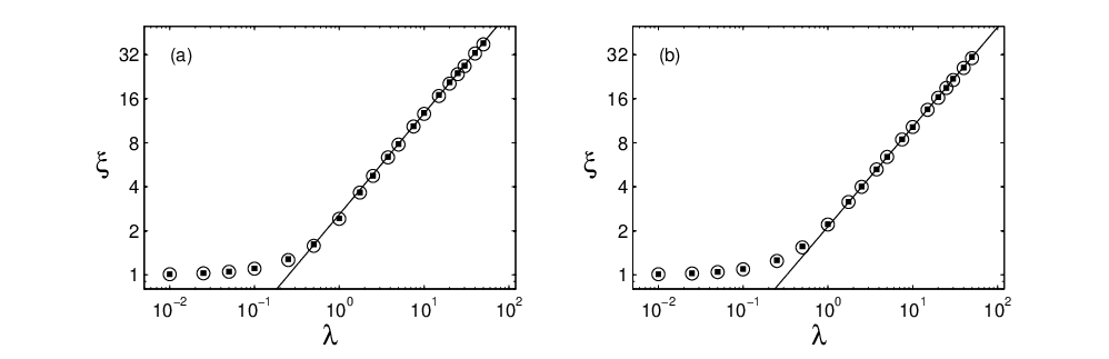
In the limit of large coupling width, the correlation length $\xi$ of the system may be defined as the average cluster mass. In Fig. 3, we plot $\xi$ as a function of $\lambda$ for rectangular and triangular distributions. For all distributions considered, the scaling

$\displaystyle\xi\sim\lambda^{\nu}$

(8)

holds for large $\lambda$, where $\nu$ is the critical exponent. Table 1 lists the values of $\nu$ for different types of distributions. In Sec. II.3, we comment on the significance of $\nu$. Note that $\lambda$ is a proxy for coupling strength, since larger $\lambda$ implies larger couplings in the system.

The RG described above is a functional RG since the decimation steps modify distributions of $\omega$, $K$, and $m$, as opposed to a small set of parameters in a uniform system [17]. The flow of the RG is given by how those distributions evolve as energy decreases. This corresponds to a coarse graining due to the buildup and removal of clusters through the decimation steps. Since there is not global synchronization in one dimension [13], clusters cannot grow forever. Indeed, by the end of the RG, the chain has been completely divided into a list of fast oscillators.

The fixed points of the functional RG are the distributions of $\omega$ and $K$ that are invariant under the flow of the RG. We identify two fixed points of the RG. The stable fixed point is given by $\lambda=0$, or $\rho_{K}(K)=\delta(K)$. This corresponds to the unsynchronized phase, since all the oscillators are freely rotating. The unstable fixed point is given by $\lambda=\infty$. This corresponds to the synchronized phase, since $\rho_{\omega}$ is then relatively narrowly peaked at zero. Any finite $\lambda$ will flow to the unsynchronized fixed point (Figs. 4 and 8). See Sec. V.1 for further discussion of the unsynchronized fixed point.

The system may be interpreted as having a phase transition at $\lambda=\infty$, similar to the transition the one-dimensional Ising model has at zero temperature. The coupling width here is analogous to inverse temperature: the system becomes more ordered as $\lambda$ increases. The scaling in Eq. (8) for large $\lambda$ probes the criticality of the system, and the correlation length $\xi$ diverges at the critical point.

It is common for equilibrium systems to exhibit universality near the critical point. This means that macroscopic quantities, such as the correlation length, scale with temperature in the same way for different systems near the critical temperature [10]. Although the model given by Eq. (1) is far from equilibrium, since it is driven and overdamped, one may still find universal behavior near the critical point. Indeed, Table 1 shows that the exponent $\nu$ is the same across different types of disorder. When $\rho_{\omega}$ and $\rho_{K}$ are rectangular, triangular, or Gaussian, $\nu\approx 2/3$, and thus those systems belong to the same universality class. On the other hand, the Lorentzian case has $\nu\approx 1/2$ and is in a different universality class.

The significance of universality is twofold. First, it means that the scaling given by $\nu$ does not depend on the microscopic details of a particular system. This is important when designing experiments to study synchronization. When it comes to observing the scaling in Eq. (8), the exact shapes of $\rho_{\omega}$ and $\rho_{K}$ are not critical, as long as they are within a given universality class. Second, from a theoretical standpoint, universality is important in that it is often closely related to the RG flow near the critical point [10]. In Sec. III, we draw the connection between universality and the RG flow. The fact that the RG correctly predicts the scaling laws boosts the claim that it is in fact a good representation of the model.

As explained in Sec. II.1, oscillators and bonds are decimated in order of decreasing energy. To simplify the analysis in this section, we define the energy of a bond to be $K$ instead of $K/2\mu$. This means that a bond may be considered for strong coupling earlier on in the RG. This makes a difference only when the bond’s $r\equiv K/\mu|\Delta\omega|>1$ when $E\equiv K$ but would have been $r<1$ when $E\equiv K/2\mu$. In practice, this happens rarely. Empirically, it is more accurate to use $K/2\mu$ as the energy, but using $K$ instead overestimates $\xi$ by only up to 5%.

When $\lambda\gg 1$, most bonds have higher energy than all the oscillators (Fig. 5). Also, most bonds will satisfy $r>1$ and will be strongly coupled. Hence, the initial stage of the RG (when $E>E^{*}$ for some $E^{*}$) is given by the strong coupling of all bonds that satisfy $K\geq E$. Since the strong coupling decimation is done independently of the $m$ and $\omega$ of the corresponding oscillators, there are no correlations between oscillators remaining in the chain. $E^{*}$ is defined as the energy scale at which the presence of fast oscillators becomes important (when $r\simeq 1$). In the remainder of this section, we calculate the RG flow for $E>E^{*}$.

Let $\rho_{m}(m,E)$ and $\rho_{K}(K,E)$ be the normalized distributions of $m$ and $K$ of the chain at a given energy $E$. As the energy is decremented from $E$ to $E-dE$, $dE\cdot\rho_{K}(E,E)$ pairs of oscillators are decimated as strongly coupled, and the corresponding couplings disappear. The flow of $\rho_{K}(K,E)$ is therefore given by simply rescaling on the interval $0<K<E$:

$\displaystyle\rho_{K}(K,E)=\frac{\rho_{K}(K,E_{0})}{\int_{0}^{E}dK^{\prime}\rho_{K}(K^{\prime},E_{0})}\;,$

(9)

where $E_{0}$ is the initial energy and $\rho_{K}(K,E_{0})$ is the initial $K$ distribution. The flow of $\rho_{m}$ is given by successively combining pairs of oscillators:

$\displaystyle\rho_{m}(m,E-dE)=\frac{\rho_{m}(m,E)+dE\,\rho_{K}(E,E)\left[-2\rho_{m}(m,E)+\int\int dm_{1}dm_{2}\rho_{m}(m_{1},E)\rho_{m}(m_{2},E)\delta(m-(m_{1}+m_{2}))\right]}{1-dE\rho_{K}(E,E)}\;,$

(10)

which leads to the integro-differential equation:

$$\frac{\partial\rho_{m}}{\partial E}=\rho_{K}(E,E)\left[\rho_{m}(m,E)-\int_{0}^{m}dm^{\prime}\rho_{m}(m^{\prime},E)\rho_{m}(m-m^{\prime},E)\right]\;.$$

(11)

We treat $m$ as a continuous variable on the range $[\,0,\infty)$. The initial condition at $E_{0}$ can be approximated by

$\displaystyle\rho_{m}(m,E_{0})=e^{-m}\;,$

(12)

which captures the fact that clusters have size one. The equation may be solved by Laplace transforming with respect to $m$. The solution is

$\displaystyle\rho_{m}(m,E)=\frac{1}{\ell(E)}e^{-m/\ell(E)}\;,$

(13)

where

	$\displaystyle\ell(E)$	$\displaystyle=$	$\displaystyle e^{-\int_{E_{0}}^{E}dE^{\prime}\rho_{K}(E^{\prime},E^{\prime})}$		(14)
		$\displaystyle=$	$\displaystyle\frac{1}{\int_{0}^{E}dK^{\prime}\rho_{K}(K^{\prime},E_{0})}$		(15)

is the average cluster mass at energy $E$. According to Eq. (13), $m$ is exponentially distributed in the initial stage of $E>E^{*}$. (The final distribution of cluster mass is not strictly exponential, as seen in Eq. (7) and Fig. 2.) Equation (15) relates energy to length scale. If $\rho_{K}(K,E_{0})$ is continuous and nonzero near $K=0$,

$\displaystyle\ell\sim\frac{\lambda}{E}\qquad\mbox{when }E\ll\lambda.$

(16)

This is the case for triangular, Gaussian, rectangular, and Lorentzian distributions, although the proportionality constants differ.

To calculate the correlation length $\xi$, we find the energy scale $E^{*}$ at which the system looks unsynchronized. It is given by the point in the RG when $\langle r\rangle\simeq 1$, since that is when the RG starts to encounter a lot of fast oscillators, which end cluster formation. Hence,

$\displaystyle E^{*}\simeq\langle\mu|\Delta\omega|\rangle\;,$

(17)

where the expectation value is over all pairs of oscillators at energy $E^{*}$. Since there are no correlations between $m$ and $\omega$ of different oscillators, we can use Eq. (13) for both oscillators in the pair. Also, an oscillator of mass $m$ has an $\omega$ given by the average of $m$ original frequencies. When $m\gg 1$, we can apply the central limit theorem, to find the distribution

$\displaystyle\rho_{m,\omega}(m,\omega,E)$

$\displaystyle=$

$\displaystyle\left(\frac{1}{\ell}e^{-m/\ell}\right)\left(\frac{1}{\sigma_{0}}\sqrt{\frac{m}{2\pi}}e^{-\frac{m\omega^{2}}{2\sigma_{0}^{2}}}\right)\;,$

(18)

where $\sigma_{0}$ is the standard deviation of the original $\rho_{\omega}$. Thus the expectation value is given by

$\displaystyle\langle\mu|\Delta\omega|\rangle$

$\displaystyle=$

$\displaystyle\int\int\int\int dm_{1}dm_{2}d\omega_{1}d\omega_{2}\,\rho_{m,\omega}(m_{1},\omega_{1},E)\,\rho_{m,\omega}(m_{2},\omega_{2},E)\,\frac{m_{1}m_{2}}{m_{1}+m_{2}}\,|\omega_{1}-\omega_{2}|\;.$

(19)

The $\ell$ and $\sigma_{0}$-dependence can be removed from the integrand by scaling the integration variables appropriately, and the resulting integral can be done numerically:

$\displaystyle\langle\mu|\Delta\omega|\rangle$

$\displaystyle=$

$\displaystyle 0.42\,\sigma_{0}\,\ell^{1/2}\;.$

(20)

The length scale at $E=E^{*}$ is given by $\ell(E^{*})\equiv\xi$. Combining Eqs. (16), (17), and (20), we find

$\displaystyle E^{*}$

$\displaystyle\sim$

$\displaystyle\xi^{1/2}\sim\left(\frac{\lambda}{E^{*}}\right)^{1/2}\;.$

(21)

Solving Eq. (21) for $E^{*}$ yields

$\displaystyle E^{*}$

$\displaystyle\sim$

$\displaystyle\lambda^{1/3}$

(22)

and thereby

$\displaystyle\xi$

$\displaystyle\sim$

$\displaystyle\lambda^{2/3}\;,$

(23)

which predicts that $\nu=2/3$ and matches simulation results (Table 1). Although the exponent is the important quantity, we note that when all proportionality constants are included, the value of $\xi$ predicted here is within 10% of the simulated result. We also note that $E^{*}$ is universal, according to Eq. (22).

The universality of $\nu$ among Gaussian, triangular, and rectangular distributions is seen to come from Eqs. (16) and (18). In other words, if $\rho_{\omega}$ has finite variance and $\rho_{K}$ is continuous and nonzero at $K=0$, then $\nu=2/3$.

Now we check when the above argument is self-consistent. We assumed that $\lambda$ is large, so that the RG does only strong coupling decimation in the beginning. Also, $\xi$ should be large so that it is valid to treat $m$ as a continuous variable, to use the central limit theorem, and so that Eq. (16) would hold at $E^{*}$. To find how large $\lambda$ should be for the power-law scaling to be accurate, we require $\xi\gg 1$ in Eq. (23) in a self-consistent way. For rectangular $\rho_{\omega}$ and $\rho_{K}$, we find the condition $\lambda\gg 0.24$. According to simulation results in Fig. 3, the power-law scaling holds for $\lambda\geq 7.5$.

One may use the above results to calculate the dynamical exponent $z$ for the system. It describes how the diverging time scale of the system scales with the diverging correlation length near criticality [18]. Intuitively, when the chain is composed of long clusters, the clusters tend to have small frequencies, so the characteristic time scale of the system is large. The characteristic frequency of the final list of clusters may be approximated by the frequency standard deviation of the original oscillators at $E^{*}$:

$\displaystyle\langle\omega^{2}\rangle_{o}$

$\displaystyle=$

$\displaystyle\frac{\int\int dm\,d\omega\,\rho_{m,\omega}(m,\omega,E^{*})\,m\,\omega^{2}}{\int dm\,\rho_{m}(m,E^{*})\,m}\;.$

(24)

The expectation value is done over the original oscillators, as opposed to clusters of oscillators, which is why the integrands include the factor $m$. In the case when Eq. (18) holds, the time scale is given by

$\displaystyle\frac{1}{\sqrt{\langle\omega^{2}\rangle_{o}}}$

$\displaystyle\sim$

$\displaystyle\xi^{1/2}\;.$

(25)

Thus, the dynamical exponent $z=1/2$ when $\rho_{\omega}$ has finite variance. This matches well with simulation results.

When $\rho_{\omega}$ is Lorentzian, $\sigma_{0}$ is infinite, so we cannot use the central limit theorem to characterize oscillator frequencies as in Eq. (18). Instead, we use the fact that the average of random variables drawn from a Lorentzian distribution is described by the same Lorentzian distribution. Thus, Eq. (18) is modified to

$\displaystyle\rho_{m,\omega}(m,\omega,E)$

$\displaystyle=$

$\displaystyle\left(\frac{1}{\ell}e^{-m/\ell}\right)\rho_{\omega}(\omega,E_{0})\;,$

(26)

so that the second factor is independent of $m$. Following the same procedure as before leads to the exponent $\nu=1/2$, which agrees well with simulations (Table 1). Note that $\nu=2/3$ if $\rho_{\omega}$ is rectangular and $\rho_{K}$ is Lorentzian.

We can extend the analysis to the case where all the couplings are equal to a constant, here denoted by $\lambda$. This is the most commonly studied case in the literature. First we consider the situation when $\rho_{K}$ is a rectangle of width $\epsilon$ at $K=\lambda$:

$\displaystyle\rho_{K}(K,E_{0})$

$\displaystyle=$

$\displaystyle\frac{1}{\epsilon}\qquad\lambda-\epsilon<K<\lambda\;.$

(27)

Equation (15) gives

$\displaystyle\ell(E)$

$\displaystyle=$

$\displaystyle\frac{\epsilon}{E-\lambda+\epsilon}\qquad\lambda-\epsilon<E<\lambda\;.$

(28)

If $\rho_{\omega}$ has finite variance, then Eq. (21) becomes

$\displaystyle E^{*}$

$\displaystyle\sim$

$\displaystyle\xi^{1/2}=\left(\frac{\epsilon}{E^{*}-\lambda+\epsilon}\right)^{1/2}\;,$

(29)

which, in the limit of $\epsilon\rightarrow 0$, leads to $\nu=2$, which is close to the simulated value 2.04(5). This agrees with the value given in [9], based on the linear approximation to Eq. (1). The critical exponent can also be predicted using the result that for a chain of size $N$, the critical coupling for complete synchronization scales as $O(\sqrt{N})$ [13, 19]. This implies that for an infinite chain, the length scale of synchronized clusters scales as $O(\lambda^{2})$.

To summarize, we have derived the scaling behavior near the synchronized fixed point by studying the RG flow. The analytical predictions for the critical exponent match closely with the results of simulations and numerical RG (Table 1). We have presented a general procedure for handling different types of distributions, and it may be applied beyond the cases considered here. For example, one may study the case where $\rho_{K}$ diverges at $K=0$, which would require the scaling in Eq. (16) to be modified.

At the unsynchronized fixed point, $\rho_{K}(K)=\delta(K)$, meaning that all the remaining oscillators are effectively uncoupled to each other. Since this fixed point is stable, at late stages of the RG, the chain will be punctured by many $K=0$ bonds (Fig. 7). This is due to the removal of a lot of fast oscillators, which leaves the former neighbors uncoupled. Due to the large fraction of $K=0$ bonds, most oscillators will be uncoupled to both neighbors. Such isolated oscillators are waiting to be removed as fast oscillators and will not be strongly coupled with their neighbors. Unless the $\omega$ distribution of isolated oscillators diverges at zero, it will approach a uniform distribution on the interval $[-E,E]$ and zero elsewhere, since the flow is given by successively chopping off the sides. Thus at the unsynchronized fixed point, $\rho_{\omega}(\omega)=\frac{1}{2E}$ for $|\omega|\leq E$. Note that these isolated, low-frequency oscillators can be clusters of mass one or of higher mass, depending on the size of $\lambda$.

Due to the stability of the unsynchronized fixed point, almost all chains will flow to it, regardless of the initial distributions of $\omega$ and $K$. Figures 8 shows examples of chains with different initial distributions flowing to the same fixed point.

Now we consider the way $\rho_{\tilde{K}}$ and $\rho_{\omega}$ approach their respective fixed distributions. We look at the component of the distributions that are not the fixed distributions. For $\rho_{\tilde{K}}$, this means considering only bonds with $\tilde{K}\neq 0$. For $\rho_{\omega}$, this means considering only oscillators with at least one nonzero bond. These components are perturbations that decay as the RG approaches the fixed point. Figures 9 show these perturbations.

It is seen that the $\tilde{K}$ perturbation collapses onto a triangular distribution regardless of the initial distributions, while the $\omega$ perturbation collapses onto a flat and quadratic shape. Hence, there is a universal approach to the stable fixed point. One can think of the fixed point as having a least negative eigenvalue, corresponding to a favored direction for approaching the fixed point in the functional RG space.

This suggests why the RG works well even with weak randomness. Regardless of whether the chain starts with strong or weak randomness, distributions of oscillator properties will look similar as the RG progresses.

In the following section, we explain how the triangular $\tilde{K}$ perturbation comes about. Due to rather technical details, we postpone the explanation of the flat-quadratic $\omega$ perturbation to the appendix.

Here, we explain how the RG algorithm leads to the universal shape of the $\tilde{K}$ perturbation. Since the perturbation is due to nonzero bonds, we consider pairs of oscillators with a nonzero bond connecting them, but otherwise uncoupled to the rest of the chain (Fig. 7). We ignore single oscillators that are uncoupled to both neighbors, since they are waiting to be removed as fast oscillators and do not contribute to the buildup of future clusters.

To facilitate the discussion, we define a center to be a pair of oscillators that both satisfy $|\omega|<E$, where $E$ is the energy of the RG at a given stage. A tail is a pair of oscillators where at least one $|\omega|>E$. In other words, neither of the oscillators in a center has been checked for fast oscillator decimation. On the other hand, at least one of the oscillators in a tail has been checked for fast oscillator decimation, but since it is still in the chain, we know that it satisfies $r>1$ and is waiting to be strongly coupled (when $E=\tilde{K}$).

A pair can stop being a center by either being checked for fast oscillator decimation or strong coupling decimation. In the first case, the pair will either be removed ($r<1$) or become a tail ($r>1$). In the second case, the pair will either be strongly coupled ($r>1$) or remain intact in the chain ($r<1$). It can be shown that when a center gets checked for strong coupling decimation, it will always be decimated [20]. It is also possible for new centers to be formed, due to the strong coupling of other oscillators; however, we can neglect this possibility when it is unlikely to have two nonzero bonds in a row.

Let the centers be described by the distribution $\rho^{c}(\omega_{1},\omega_{2},\tilde{K};E)$, where $|\omega_{1}|>|\omega_{2}|$. This distribution is nonzero only when $|\omega_{1}|,\tilde{K}<E$. Its flow is given by setting to zero the region that doesn’t satify that inequality, and then normalizing to unity. Unless there is a divergence at the origin, the distribution of centers approaches

$$\rho^{c}(\omega_{1},\omega_{2},\tilde{K};E)=\frac{1}{2E^{3}}\quad\quad|\omega_{2}|<|\omega_{1}|<E,0<\tilde{K}<E\;.$$

(38)

This is just the statement that any smooth distribution will look flat if you keep chopping off its sides. Integrating out $\omega_{1},\omega_{2}$ in Eq. (38), we find that the distribution of $\tilde{K}$ of centers is flat:

$\displaystyle\rho^{c}_{\tilde{K}}(\tilde{K};E)$

$\displaystyle=$

$\displaystyle\frac{1}{E}\quad\quad 0<\tilde{K}<E\;.$

(39)

We now consider centers at the moment they get checked for fast oscillator decimation, i.e. when $\omega_{1}=E$. Here we assume that $\omega_{1}$ is positive, but analogous results hold for when it is negative.

$$\rho^{c}_{\omega_{1}=E}(\omega_{2},\tilde{K};E)=\frac{1}{2E^{2}}\quad\quad 0<|\omega_{2}|,\tilde{K}<E\;$$

(40)

At this point, if $\omega_{2}$ and $\tilde{K}$ are such that $r<1$, then oscillator 1 will get removed as a fast oscillator, and oscillator 2 will become an isolated oscillator, which is then ignored. But if $r>1$, then the pair becomes a tail and remains in the chain. Thus the new tails at energy E are described by:

$$\rho^{t}_{\omega_{1}=E}(\omega_{2},\tilde{K};E)=\frac{1}{E^{2}}\quad\quad 0<\frac{|\omega_{2}-E|}{2}<\tilde{K}<E\;,$$

(41)

which can be rewritten as

$$\rho^{t}_{\omega_{1}=E}(|\Delta\omega|,\tilde{K};E)=\frac{1}{E^{2}}\quad\quad 0<\frac{|\Delta\omega|}{2}<\tilde{K}<E\;.$$

(42)

This distribution is constant over a triangular region in $|\Delta\omega|$, $\tilde{K}$ as illustrated in Fig. 10.

Now here is the key. Tail pairs remain in the chain until they are decimated as strongly coupled, which happens when the RG energy reaches the bond energy. Thus Eq. (42) describes the flow of the existing tails at any energy $E$. Existing tails have the same distribution as incoming tails at any energy, so Eq. (42) describes all tails.

By integrating out $|\Delta\omega|$ in Eq. (42), one finds that the $\tilde{K}$ distribution of tails is triangular:

$\displaystyle\rho^{t}_{\tilde{K}}(\tilde{K};E)$

$\displaystyle=$

$\displaystyle\frac{2}{E^{2}}\;\tilde{K}\quad\quad 0<\tilde{K}<E\;.$

(43)

In principle, the combined $\tilde{K}$ distribution of center and tail pairs is given by a weighted average of Eqs. (39) and (43). But it is shown in the appendix that as energy decreases, there are more and more tails relative to centers, so that at low energy, all non-zero $\tilde{K}$ are given by just Eq. (43). This explains the triangular distribution in Fig. 9.

The universality of Eq. (43) comes from the applicability of Eq. (38). Unless $\rho_{\omega}$ diverges at $\omega=0$, $\rho_{\tilde{K}}$ will approach $\delta(\tilde{K})$ through a decaying triangular perturbation as energy decreases. This explains the universal approach to the stable fixed point.

The above discussion has focused on RG flow at low energies, which corresponds to low frequency clusters. When $E$ is sufficiently small, Eq. (38) accurately describes centers. In physical terms, Eq. (38) describes pairs of clusters with $|\omega_{1}|,|\omega_{2}|<E$ that are interacting via a bond $\tilde{K}$. Depending on how big the coupling is, the two clusters may end up synchronizing and forming a bigger cluster.

Most of the clusters with $|\omega|<E$ will be effectively isolated from the rest of the chain, since most couplings are zero at low energy. It is shown in the appendix that of the cluster pairs that are coupled and have at least one cluster with $|\omega|<E$, 3/5 are centers and 2/5 are tails. The centers have interactions given by Eq. (39), while tails have interactions given by (43). Since Eqs. (38) and (43) and the proportion of centers and tails are universal across different initial distributions, we know that the dynamics at low frequency are also universal. Thus, this analysis of the RG provides insight into the interactions of low frequency clusters.

A possible extension of this analysis is to study the distribution of cluster mass. As mentioned in Sec. II.2, the final distribution of cluster mass is of the form in Eq. (7). In the current discussion, the mass information is stored in the bond energy $K/2\mu$. We have considered the flow of pairs of oscillators that are uncoupled from the rest of the chain. By considering the flow of longer isolated chains, one may be able to understand the buildup of larger clusters and hence the final mass distribution. The difficulty lies in the correlations that appear due to the $r$ criterion.

References

- [1] Y. Kuramoto, Chemical Oscillations, Waves, and Turbulence (Springer-Verlag, Berlin, 1984).
- [2] A. S. Pikovsky, M. Rosenblum, and J. Kurths, Synchronization: A Universal Concept in Nonlinear Science (Cambridge University Press, New York, 2001).
- [3] J. A. Acebrón, L. L. Bonilla, C. J. P. Vicente, F. Ritort, and R. Spigler, Rev. Mod. Phys. 77, 137 (2005).
- [4] K. Wiesenfeld, P. Colet, and S. H. Strogatz, Phys. Rev. Lett. 76, 404 (1996).
- [5] A. G. Vladimirov, G. Kozyreff, and P. Mandel, Europhys. Lett. 61, 613 (2003).
- [6] F. Varela, J.-P. Lachaux, E. Rodriguez, and J. Martinerie, Nature Reviews Neurosci. 2, 229 (2001).
- [7] Z. Néda, E. Ravasz, Y. Brechet, T. Vicsek, and A.-L. Barabási, Nature 403, 849 (2000).
- [8] H. Hong, H. Park., and M. Y. Choi, Phys. Rev. E 72, 036217 (2005).
- [9] H. Hong, H. Chaté, H. Park., and L.-H. Tang, Phys. Rev. Lett. 99, 184101 (2007).
- [10] N. Goldenfeld, Lectures on Phase Transitions and the Renormalization Group (Westview Press, Boulder, CO, 1992).
- [11] H. Sakaguchi, S. Shinomoto, and Y. Kuramoto, Prog. Theor. Phys. 77, 1005 (1987).
- [12] H. Daido, Phys. Rev. Lett. 61, 231 (1988).
- [13] S. H. Strogatz and R. E. Mirollo, J. Phys. A 21, L699 (1988).
- [14] O. Kogan, J. L. Rogers, M. C. Cross, and G. Refael, accepted for publication in Phys. Rev. E, arXiv:0810.3075.
- [15] O. Kogan, Ph.D. thesis, California Institute of Technology (2008).
- [16] W. H. Press, B. P. Flannery, S. A. Teukolsky, and W. T. Vetterling, Numerical Recipes in C: The Art of Scientific Computing (Cambridge University Press, Cambridge, 1992).
- [17] D. Fisher, Phys. Rev. B 50, 3799 (1994).
- [18] S. L. Sondhi, S. M. Girvin, J. P. Carini, and D. Shahar, Rev. Mod. Phys. 69, 1 (1997).
- [19] J. Ochab and P. F. Góra, submitted to Acta Phys. Pol. B, arXiv:0909.0043.
- [20] By the definition of a center, . When a center gets checked for strong coupling decimation, . Thus, . Hence, when a center is checked for strong coupling decimation, it will always be decimated as such.